BIFURCATION THEORY APPLIED TO THE ANALYSIS OF POWER SYSTEMS
GUSTAVO REVEL, DIEGO M. ALONSO, AND JORGE L. MOIOLA
Abstract. In this paper, several nonlinear phenomena found in the study of power system networks are described in the context of bifurcation theory. Toward this end, a widely studied 3-bus power system model is considered. The mechanisms leading to static and dynamic bifurcations of equilibria as well as a cascade of period doubling bifurcations of periodic orbits are in-vestigated. It is shown that the cascade verifies the Feigenbaum’s universal theory. Finally, a two parameter bifurcation analysis reveals the presence of a Bogdanov-Takens codimension-two bifurcation acting as an organizing cen-ter for the dynamics. In addition, evidence on the existence of a complex global phenomena involving homoclinic orbits and a period doubling cascade is included.
1. Introduction
Power systems blackouts have received a great attention in the last few years, due to the increasing amount of incidents occurred in many countries around the world (see for example [17,20,3,27] and references therein). For different reasons many systems are forced to operate near to their stability limits and thus they are vulnerable to perturbations of the operating conditions. When these limits are ex-ceeded, the system can exhibit undesired transient responses with the impossibility to retain a stable voltage profile. This phenomenon is known as voltage collapse. Factors that influence it are increments in the load consumption that reach the limits of the network or the generation capacity, actions of badly tuned controllers, tripping of lines and generators, among others [6].
Power system networks are one of the more complex and difficult systems to model. The first problem is the size, just imagine a large-scale network composed by hundreds of generators connected by thousands of transmission lines and buses, along with probably hundreds of load centers, as it is easy to find in almost every country. A second problem is its complex nature. Physical variables with very different time scales (the electrical variables are sometimes extremely faster than the mechanical states of the generators), devices modelled by continuous dynamics (generators, loads, etc.) combined with discrete events (faults, controllers, etc.),
Key words and phrases. nonlinear systems, power systems, voltage collapse, numerical analy-sis, bifurcations, chaos.
algebraic restrictions (network constraints, operating conditions, etc), are some of the main features revealing the complexity of the system. Therefore, to deal with a tractable model it is necessary to make simplifications such as replacing a group of generators, lines and/or loads for a single device with an equivalent behavior, or neglecting fast dynamics, etc. By far, the usual approach to model a power system is using a differential-algebraic set of equations (DAE model) of the form [13, 23]
˙
x = f(x, y;λ),
0 = g(x, y;λ),
where f : Rn×m×p →Rn, g :Rn×m×p →Rm, x∈Rn represents the differential
or dynamical state variables,y∈Rm represents the algebraic state variables, and λ∈ Rp is a vector of real parameters. The differential variables include the
me-chanical states of the generators (swing equations), the electrical states of the rotor, the excitation and governor systems (voltage and frequency controls, respectively) and the dynamical states of the load. On the other hand, the algebraic states are mainly determined by the transmission network and algebraic states of the gener-ators stgener-ators and loads∗. It is easy to obtain a high dimensional DAE model from a real power system. For example, a widely studied system corresponding to the Western System Coordinating Council (WSCC) composed by three machines and nine buses [2,19,23], is modelled with 45 equations, 21 differential and 24 algebraic. The total number of equations might vary according to the detail used when mod-elling generators and loads. A more complete model results from considering an hybrid system which is described by a set of differential-algebraic-difference (DAD) equations [11], to accurately include faults and the discrete nature of some compo-nents of the system. Nevertheless, it is important to notice that the complexity of the model depends on the problem under study.
In addition, power systems are highly nonlinear and its dynamical behavior may change qualitatively when parameters are varied. For example, after a load increment a stable operating point may become unstable and oscillations arise. This behavior can be locally associated to a Hopf bifurcation and, in general, bifurcation theory can be applied to understand mechanisms leading to nonlinear phenomena in these systems. The idea underlying a bifurcation analysis is to investigate qualitative changes in the system dynamics (e.g. stability loss, birth or death of oscillations, passage from periodic to chaotic solutions or viceversa, etc.) underslow variations of distinctive system parameters. In this regard, [1] and [15] present results in the study of steady state stability of power systems considering dynamic (Hopf) and static (saddle-node) bifurcations, respectively. Then, Dobson and Chiang [5] have introduced a simple 3-bus power system model showing that the interaction between the load and generator causes a saddle-node bifurcation. As
∗The algebraic states arise from neglecting the dynamics of lines (instantaneous power
Figure 1. Schematic diagram of the 3-bus electric power system model.
a consequence the stable operating point disappears if the reactive power demand is increased and then the voltage on the load suddenly drops to zero (voltage collapse). This simple model has been widely studied using different sets of parameter values (e.g. [29, 26,16, 4]). For example, Wang et al. [29] have shown that this system can develop a voltage collapse following a cascade of period doubling bifurcations. Later, Budd and Wilson [4] have found a Bogdanov-Takens bifurcation point when considering two parameter variations.
In this paper, the 3-bus power system model is revisited. An overview of bifurca-tions when varying one and two parameters is presented. It is shown that in a one parameter bifurcation analysis, saddle-node and Hopf bifurcations of equilibria are the mechanisms by means an operating point can disappear or become unstable, respectively. In addition, the periodic orbit born at the Hopf bifurcation under-goes a cascade of period doubling bifurcations leading to a chaotic attractor. It is shown that the cascade follows the theory proposed by Feigenbaum [8, 9]. When considering variations of two parameters, a Bogdanov-Takens codimension two bi-furcation point is detected for positive values of the active and reactive power of the load. Even though the unfolding of this bifurcation seems not to affecta priori the operating point of the system, the appearance of additional global phenomena can influence the behavior over regions of practical importance.
This paper is organized as follows. In section 2 the model of the power system is described. One and two parameter bifurcation analysis are developed in sections 3 and 4, respectively. Finally, in section 5 some concluding remarks are presented.
2. Mathematical model of a 3-bus electric power system
The 3-bus power system model introduced in [5] and shown in Fig. 1, consists of an infinite bus on the left, a load bus on the center and a generator bus on the right.
Y0∠(−θ0−π/2) andYm∠(−θm−π/2) are the admittances of the transmission lines. The concept of an infinite bus refers to a particular node of the system with enough capacity to absorb any mismatch in the power balance equations. Thus, it can be considered as a fictitious generator with constant voltage magnitudeE0
other hand, the generator has constant voltage magnitude Em but the angle δm
varies according to the so-called swing equation
M¨δm+dmδm˙ =Pm−Pe, (2.1)
where M is the inertia of the rotor, dm is the damping coefficient, Pm is the mechanical power supplied to the generator andPe is the electric power supplied by the generator to the network (including the loss inYm) given by
Pe=−EmYm[Emsin(θm) +V sin(δ−δm+θm)]. (2.2)
Replacing (2.2) in (2.1), the dynamics of the generator is reproduced by theclassical model of a voltage generator (also known asconstant voltage behind reactance [24])
˙
δm = ω (2.3)
˙
ω = 1
M
−dmω+Pm+E2
mYmsin(θm) +EmV Ymsin(δ−δm+θm)
.(2.4)
The load bus, with voltage magnitude V and phase δ, consists of an induction motor, a generic load P-Q and a capacitorC. The dynamics of this part is derived from a power balance at the bus. Considering an empirical model for the induction motor [28] and a static load P-Q, the power consumption results
Pload = P0+kpwδ˙+kpv(V +TV˙)
| {z }
Pmotor
+P1,
Qload = Q0+kqwδ˙+kqvV +kqv2V2
| {z }
Qmotor
+Q1,
where T, kpw, kpv, kqw, kqv andkqv2 are constants of the motor,P0,Q0 andP1,
Q1 are the static active and reactive power drained by the motor and by the load P-Q, respectively. In terms of bus voltages and lines admittances, the active and reactive power supplied to the load are
P(δm, δ, V) = −E0′Y0′Vsin(δ+θ0′)−EmYmV sin(δ−δm+θm) +V2hY′
0sin(θ ′
0) +Ymsin(θm)
i
, (2.5)
Q(δm, δ, V) = E0′Y ′
0Vcos(δ+θ ′
0) +EmYmVcos(δ−δm+θm) −V2hY′
0cos(θ ′
0) +Ymcos(θm)
i
, (2.6)
whereE0′,Y ′ 0 andθ
′
0are obtained from a Thevenin equivalent of the circuit towards
the infinite bus including the capacitorC, and their expressions are
E0′ = E0
Γ , Y
′
0 =Y0Γ, θ ′
0=θ0+ tan−1
CY−1
0 sin (θ0)
1−CY0−1cos (θ0)
,
with Γ =q1 +C2Y−2
Then the balance between the supplied power (P, Q) and the drained power (Pload,Qload) at the load bus results in
P(δm, δ, V) = P0+kpwδ˙+kpv(V +TV˙) +P1, (2.7)
Q(δm, δ, V) = Q0+kqwδ˙+kqvV +kqv2V
2+Q1. (2.8)
From (2.8)
˙
δ= 1
kqw
−kqv2V2−kqvV −Q0−Q1+Q(δm, δ, V). (2.9)
Substituting (2.9) into (2.7) and solving for ˙V, results
˙
V = 1
T kqwkpv
kpwkqv2V2+ (kpwkqv−kqwkpv)V (2.10)
+kqw[P(δm, δ, V)−P0−P1]−kpw[Q(δm, δ, V)−Q0−Q1]}.
Equations (2.3–2.4) and (2.9–2.10) withP(·) andQ(·) given by (2.5) and (2.6), respectively, describe the dynamics of the 3-bus system model in terms of the state variables δm, ω, δ, and V. The free parameters used in the bifurcation analysis areQ1 andP1, i.e. the reactive and active power drained by the static P-Q load. Therefore the model has the form
˙
x=f(x, λ) (2.11)
where x = [δm, ω, δ, V]T is the state vector and λ = [Q1, P1]T is the parameter
vector. The values of the fixed parameters used in the following numerical study are obtained from [29]: M = 0.01464,C= 3.5,Em= 1.05,Y0= 3.33,θ0=θm= 0,
kpw = 0.4, kpv = 0.3, kqw =−0.03, kqv = −2.8, kqv2 = 2.1, T = 8.5,P0 = 0.6,
Q0 = 1.3, E0 = 1, Ym = 5.0, Pm = 1.0 and dm = 0.05. All the constants are normalized according to a given basis (“per-unit” representation), except for the angles which are given in degrees.
3. One parameter bifurcation analysis
Let us denote the 3-bus power system operation point asx∗= [δ∗
m, ω∗, δ∗, V∗]T,
which is normally a stable equilibrium of (2.11) for someλ, i.e. f(x∗, λ) = 0. The
location ofx∗changes as the parameter vectorλvaries. In addition, the qualitative
dynamical behavior in the neighborhood ofx∗, may change at particular values of λ, sayλ=λ∗. At these points, system (2.11) undergoes local bifurcations and the
Jacobian matrix
J = ∂f
∂x(x
∗, λ∗) (3.1)
becomes singular. Considering variations of only one parameter and assuming that some nondegeneracy conditions hold, the equilibrium point x∗ exhibits a
Figure 2. Bifurcation diagram varyingQ1withP1= 0.
bifurcation. The equilibrium changes the stability and a limit cycle (oscillation) is created in its neighborhood. Further details on the analysis of different bifurcations can be seen, for example in [10] and [14].
In the following one parameter bifurcation analysis, the load reactive powerQ1
is the free parameter while the active power is fixed at P1 = 0. The analysis is performed numerically with the continuation package AUTO [7]. In this setting the equilibrium curve is computed as the main bifurcation parameter is varied and, simultaneously, bifurcation conditions are checked. Figure 2 shows the resulting bifurcation diagram. The curve is denoted as a solid line when the equilibrium is stable and dashed when it is unstable. The value of the state variable V at equilibrium is shown in the ordinate axis. In addition, the minimum value of the amplitude of the periodic orbit born at the Hopf bifurcation is plotted. Filled circles mean stable periodic orbits and empty circles denote unstable ones.
Beginning from the left in Fig. 2, there are two equilibrium points, one stable (where the system may operate) and the other unstable. The stable one becomes unstable at a supercritical Hopf bifurcation (H−) for Q1 = 2.9802182780
lead-ing to the appearance of a stable limit cycle. For increaslead-ing values of Q1, both equilibria approach each other and coalesce in a saddle-node bifurcation (SN1) for
Figure 3. Detailed view of the sequence of period doubling bifurcations.
Nevertheless, voltage collapse may be found below this point due to a more complex phenomenon [29] described next.
The cycle born at the Hopf bifurcation (H−) undergoes a cascade of period
doubling bifurcations, i.e. the period of the orbit is doubled repeatedly. This sin-gularity can not be detected from a local analysis around the equilibrium point. Nevertheless, local bifurcations of limit cycles can be detected analyzing the eigen-values of the associated Poincar´e map. When a single eigenvalue crosses the unit circle through 1 or−1, a saddle-node or a period doubling bifurcation of limit cy-cles arises, respectively. When a pair of eigenvalues cross the unit circle ate±j2π/k
withk6= 0,1, ...4†, the cycle evidences a Neimark-Sacker or secondary Hopf bifur-cation, leading to quasiperiodic motions. In the 3-bus power system under study, the first period doubling bifurcation (PD1) occurs atQ1= 2.9889650564. At this point, a stable period-two cycle is created, coexisting with the original period-one cycle, now unstable. This cycle becomes unstable at PD2 and a period-four cycle arises. The beginning of the cascade is shown in Fig. 3which is the blow-up of the rectangle of Fig. 2(the corresponding values ofQ1can be obtained from Table1). This process continues for increasing values ofQ1and leads to a chaotic attractor. A projection of this attractor forQ1= 2.989790 is depicted in Fig. 4.
†This condition avoids more complex scenarios known asstrong resonances(see, for example
Table 1. Period doubling bifurcations.
Bifurcation Q1
PD1 2.9889650564
PD2 2.9894727221
PD3 2.9895623607
PD4 2.9895809828
PD5 2.9895849451
PD6 2.9895857918
PD7 2.9895859732
−1 −0.5
0 0.5
1 −0.2
−0.1
0 0.1
0.2 0.75
0.8 0.85 0.9
ω δ
V
Figure 4. Chaotic attractor forQ1= 2.989790.
The attractor, and the associated unstable orbits, collide with the saddle equi-librium point forQ1≃2.996 and they are destroyed due to boundary crisis bifur-cations. Therefore when the chaotic attractor coalesces, the system does not have any stable attractor and the voltage collapse occurs, more precisely after a long chaotic transient the voltage drops to zero suddenly.
3.1. Analysis of the period doubling route to chaos. For unimodal maps, the values of the parameter where the period doubling bifurcations occur are related by a universal constant due to M. J. Feigenbaum [8,9] given by:
δF = lim
n→∞
rn+1−rn
Figure 5. Unimodal Lorenz’s map for ¯δm.
where rj are the parameter values corresponding to the period doubling bifurca-tions. These results may be approximately applied to ordinary differential equa-tions if the associated Lorenz’s map is unimodal [25].
Extending this idea to the power system model, the Lorenz’s map is obtained numerically by plotting the successive local maxima of the state variableδmwhen the system is in chaotic regime. The plot, shown in Fig. 5, is very close to a one dimensional curve and can be approximated by an unimodal map. Then, successive approximations to Feigenbaum’s universal constant (fornfinite) can be computed using
δF n= rn+1−rn
rn+2−rn+1
and the values of Q1 given in Table 1. The resulting approximations are given in Table 2. Notice that the estimation approaches δF = 4.6692016091...as n is increased. Thus, knowing the values ofQ1for the first period doubling bifurcations (i.e. PD1, PD2, PD3, etc.) the occurrence of the remaining bifurcation points can be approximately predicted usingδF. For example, PD8 can be predicted using
Table 2. Approximated values of Feigenbaum’s universal constant.
n δF n
1 5.663471986396961 2 4.813560232131420 3 4.699820811612138 4 4.679697647450078 5 4.667585450683690
4. Two parameter bifurcation analysis
Suppose that an equilibrium point or a limit cycle of system (2.11) undergoes a bifurcation forλ=λ∗ when variations of one parameter are considered. Then,
varying a second parameter simultaneously, there exists a curve in the parameter plane along which this bifurcation persists. At isolated points on this curve of codimension-one bifurcations, system (2.11) can exhibit codimension-two bifurca-tions. This situation corresponds to an additional linear degeneracy, either in the Jacobian matrix for equilibrium points or in the Poincar´e map for cycles.
When considering simultaneous variations of Q1 and P1 a double linear de-generation condition is detected. This condition corresponds to the double-zero or Bogdanov-Takens codimension-two bifurcation and the Jacobian (3.1) presents two eigenvalues at zero. The normal form of this bifurcation is given by
˙
x = y+O|x, y|3,
˙
y = µ1+µ2x+x2+sxy+O|x, y|3,
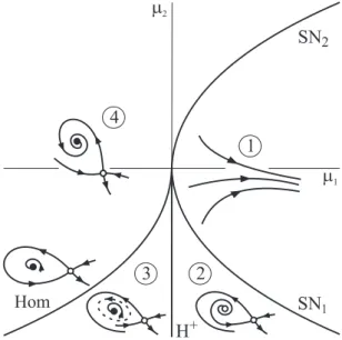
whereµ1 and µ2are the main bifurcation parameters and s=±1. The unfolding of this bifurcation for s = 1 is shown in Fig. 6 (the case s= −1 is very similar and can be seen in [14]). In region 1 there are no equilibria and crossing the curve SN1 towards region 2, two unstable equilibria are created due to a saddle-node bifurcation. Then the unstable node undergoes a subcritical Hopf bifurcation at the curve H+and becomes stable surrounded by an unstable limit cycle in region 3.
This cycle is destroyed at the homoclinic bifurcation curve Hom. The stable node and unstable saddle equilibria of region 4 collapse at the saddle-node bifurcation curve SN2.
Figure 6. Unfolding of the Bogdanov-Takens bifurcation.
Let us describe in detail the bifurcation diagram of Fig. 7. The curves associated to the Bogdanov-Takens singularity are: the two branches of static saddle-node bi-furcations (SN1 and SN2), the subcritical Hopf bifurcation (H+) and the homoclinic
bifurcation (Hom). These curves are shown in the expanded view of the rectangle of Fig. 7and correspond to those predicted in the unfolding of Fig. 6. The curves PD1 and H− are not directly related to this unfolding and deserve a particular
description. The subcritical Hopf bifurcation curve emanating from the BT singu-larity becomes supercritical (H−) at a generalized Hopf bifurcation. A cyclic fold
2.9750 2.99 3.005 3.02 3.035 0.05
0.1 0.15 0.2
Q 1 P
1
H−
H+ Hom
Hom
SN1 SN2
PD1
BT
3.0275 3.0297 3.032
0.13 0.15 0.17
H+ Hom
SN1 SN2
BT
Figure 7. Two parameter bifurcation diagram.
horizontal cross-section atP1= 0 in Fig. 7. The period doubling curves associated to the cascade are not shown in this figure but they are located within the region enclosed by the locus of PD1 and that of Hom. Additional bifurcation phenomena on a larger region of the parameter plane, as well as vertical cross-sections (fixing
Q1 and varyingP1) can be consulted in [21].
5. Conclusions
models of power systems. The existence of global nonlinear phenomena restricting the basin of attraction of the operating point can also be expected.
References
1. E. H. Abed and P. P. Varaiya,Nonlinear oscillations in power systems, Int. J. Electric Power and Energy Systems6(1984), no. 1, 37–43.1
2. P. M. Anderson and A. A. Fouad,Power system control and stability, IEEE PRESS Power System Engeneering Series, New York, 1994.1
3. G. Andersson, P. Donalek, R. Farmer, N. Hatziargyriou, I. Kamwa, P. Kundur, N. Martins, J. Paserba, P. Pourbeik, J. Sanchez-Gasca, R. Schulz, A. Stankovic, C. Taylor, and V. Vittal,
Causes of the 2003 major grid blackouts in North America and Europe, and recommended means to improve system dynamic performance, IEEE Trans. Power Systems20(2005), no. 4, 1922–1928.1
4. C. J. Budd and J. P. Wilson,Bogdanov-Takens bifurcation points and ˘Sil’nikov homoclinicity in a simple power-system model of voltage collapse, IEEE Trans. Circuits Systems I43(2002), no. 5, 575–590.1,4
5. I. Dobson and H. D. Chiang,Towards a theory of voltage collapse in electric power systems, Systems Control Lett.13(1989), no. 3, 253–262.1,2
6. I. Dobson, T. Van Cutsem, C. Vournas, C. L. DeMarco, M. Venkatasubramanian, T. Overbye, and C. A. Ca˜nizares,Voltage stability assessment: Concepts, practices and tools, ch. 2, IEEE Power Engineering Society, SP101PSS, August 2002.1
7. E. J. Doedel, R. C. Paffenroth, A. R. Champneys, T. F. Fairgrieve, Yu. A. Kuznetsov, B. E. Oldeman, B. Sandstede, and X.-J. Wang,AUTO2000: Continuation and bifurcation software for ordinary differential equations (with HomCont), Tech. report, Caltech, California, 2002.
3
8. M. J. Feigenbaum, Qualititative universality for a class of nonlinear transformations, J. Statist. Phys.19(1978), 25–52.1,3.1
9. ,The universal metric properties of nonlinear transformations, J. Statist. Phys.21 (1979), 669–706.1,3.1
10. J. Guckenheimer and P. Holmes,Nonlinear oscillations, dynamical systems, and bifurcations of vector fields, Springer Verlag, New York, 1993.3
11. D. J. Hill, Y. Guo, M. Larsson, and Y. Wang, Global control of complex power systems, Bifurcation Control (G. Chen, D. J. Hill, and X. Yu, eds.), Lecture Notes in Control and Information Sciences, vol. 293, Springer-Verlag, 2003, pp. 155–187.1
12. M. Ili´c and J. Zaborszky,Dynamics and control of large electric power systems, John Wiley & Sons, Inc, New York, 2000.∗
13. P. Kundur,Power system stability and control, McGraw-Hill, New York, 1994.1
14. Yu. A. Kuznetsov,Elements of applied bifurcation theory, Springer-Verlag, New York, 1995.
3,†,4
15. H. G. Kwatny, A. K. Pasrija, and L. Y. Bahar,Static bifurcations in electric power networks: loss of steady-state stability and voltage collapse, IEEE Trans. Circuits Systems I33(1986), no. 10, 981–991.1
16. A. H. Nayfeh, A. M. Harb, and C. M. Chin,Bifurcations in a power system model, Int. J. of Bifurcation and Chaos6(1996), no. 3, 497–512.1
17. D. Novosel, M. M. Begovic, and V. Madani,Shedding light on blackouts, IEEE Power and Energy Magazine2(2004), no. 1, 32–43.1
19. M. A. Pai, P. W. Sauer, B. C. Lesieutre, and R. Adapa,Structural stability in power systems-effect of load models, IEEE Trans. Power Systems10(1995), no. 2, 609–615.1
20. L. Pereira,Cascade to black, IEEE Power and Energy Magazine2(2004), no. 3, 54–57.1 21. G. Revel, D. M. Alonso, and J. L. Moiola,Bifurcation analysis in a power system model, First
IFAC Conf. on Analysis and Control of Chaotic Systems (Reims, France), 2006, pp. 315–320.
4
22. W. D. Rosehart and C. A. Ca˜nizares,Elimination of algebraic constraints in power system studies, IEEE Canadian Conf. on Electrical and Computer Engineering2(1998), 685–688.∗ 23. P. W. Sauer and M. A. Pai,Power system dynamics and stability, Prentice Hall, New Jersey,
1998.1
24. IEEE Power Engineering Society,IEEE guide for synchronous generator modeling practices and applications in power system stability analyses, IEEE Std 1110.-2002 (2003), 1–72.2
25. S. H. Strogatz,Nonlinear dynamics and chaos, Addison-Wesley, Reading, MA, 1994.3.1
26. C. W. Tan, M. Varghese, P. Varaiya, and F. F. Wu,Bifurcation, chaos, and voltage collapse in power systems, Proc. IEEE83(1995), no. 11, 1484–1496.1
27. C. D. Vournas, V. C. Nikolaidis, and A. A. Tassoulis,Postmortem analysis and data validation in the wake of the 2004 Athens blackout, IEEE Trans. Power Systems21(2006), no. 3, 1331– 1339.1
28. K. Walve,Modelling of power system components at severe disturbances, International Conf. on Large High Voltage Electric Systems (CIGR´E), 1986, pp. 1–9.2
29. H. O. Wang, E. H. Abed, and A. M. Hamdan, Bifurcations, chaos, and crises in voltage collapse of a model power system, IEEE Trans. Circuits Systems I41(1994), no. 3, 294–302.
1,2,3
Gustavo Revel
Instituto de Investigaciones en Ingenier´ıa El´ectrica (UNS–CONICET) Depto. de Ing. El´ectrica y de Computadoras,
Universidad Nacional del Sur, Avda. Alem 1253, B8000CPB Bah´ıa Blanca, Argentina.
Diego M. Alonso
Instituto de Investigaciones en Ingenier´ıa El´ectrica (UNS–CONICET) Depto. de Ing. El´ectrica y de Computadoras,
Universidad Nacional del Sur, Avda. Alem 1253, B8000CPB Bah´ıa Blanca, Argentina.
Jorge L. Moiola
Instituto de Investigaciones en Ingenier´ıa El´ectrica (UNS–CONICET) Depto. de Ing. El´ectrica y de Computadoras,
Universidad Nacional del Sur, Avda. Alem 1253, B8000CPB Bah´ıa Blanca, Argentina.