Imports and welfare: variety losses of the Argentine crisis of 2001-2002

(1)

IMPORTS AND WELFARE: VARIETY LOSSES OF THE ARGENTINE CRISIS OF 2001-2002

IRENE BRAMBILLA AND ROMINA TOMÉ

RESUMEN

El acceso a una mayor variedad de productos es una de las fuentes principales de ganancias del comercio internacional y la globalización. Cuando una economía atraviesa una crisis, la demanda agregada se reduce resultando en una menor variedad de productos importados. En este estudio cuantificamos las pérdidas de bienestar de corto y mediano plazo que resultan de la reducción en el número de variedades importadas durante la crisis Argentina de 2001-2002. Encontramos que a corto plazo las pérdidas de bienestar varían significativamente entre productos y que la recuperación a mediano plazo depende de la habilidad de sustituir hacia nuevas variedades.

Clasificación JEL: F10, F14

Palabras Clave: Ganancias de comercio, Variedades de producto, Crisis

Argentina.

ABSTRACT

The access to a large variety of products is one of the main sources of gains from international trade and globalization. When an economy goes through a crisis, aggregate demand shrinks resulting in fewer product varieties being imported. In this paper we quantify short-run and medium-run welfare losses that resulted from the reduction in the number of imported product varieties during the Argentine crisis of 2001-2002. We find that short-run welfare losses vary widely across products and that medium-run recovery depends on the ability to substitute towards new varieties.

JEL Classification: F10, F14

(2)

IMPORTS AND WELFARE: VARIETY LOSSES

OF THE ARGENTINE CRISIS OF 2001-2002

IRENE BRAMBILLA*_{AND ROMINA TOMÉ}*

I. Introduction

The access to a large variety of products is one of the main sources of gains from international trade and globalization. In the early theoretical models of international trade with product differentiation and fixed costs, such as Krugman (1979, 1980), the total number of available products depends on the size of world markets and are the same for all countries. In more recent models that introduce heterogeneity across firms and costs of entry into export markets, namely Melitz (2003), Helpman, Melitz and Yeaple (2004), and extensions thereafter, firms can decide to enter some markets but not others. As a result, some products are not available in smaller economies.1_{From a}

dynamic viewpoint, market size and aggregate demand fluctuate. In particular, when an economy goes through a macro crisis that shrinks aggregate demand, the number of available product varieties goes down, resulting in a welfare loss for consumers.2

In this paper we quantify short-run and medium-run welfare losses that resulted from the reduction in the number of imported product varieties during

*_{Universidad Nacional de La Plata, Departamento de Economía, Calle 6 e 47 y 48, 1900 La}

Plata, Argentina. email: [email protected]

*_{Inter-American Development Bank, 1300 New York Avenue, NW, Washington DC, 20577.}

email: [email protected]

1_{The mechanism works through revenue and fixed costs. In smaller economies the possibilities}

of revenue are smaller and thus it becomes harder to cover the fixed costs of entry to that market. The relatively more inefficient firms, for which revenue is lower than for their more efficient competitors, decide not to enter. Notice that since firms produce a single differentiated product, firms and products are equivalent.

2_{We can think of consumer preferences as being of “love of variety”’ or “ideal variety”}_{type. In}

(3)

the Argentine crisis of 2001-2002. After almost a decade of currency board during which the peso was pegged one to one to the dollar, Argentine GDP growth started to decline in the late 1990s leading to a big recession and financial collapse. In December 2001 bank deposits were frozen (the so called “corralito”) and in January 2002 Argentina defaulted its external debt. During the first few months of 2002, the Argentine peso depreciated by 300 percent. The crisis took a big toll on imports. Total value of imports dropped by 65 percent between 2000 and 2002, from 23 to 8 billion dollars. Together with a reduction in the total value of imports, there was also a reduction in the number of imported products and in the number of countries from which each product was imported. Customs data show that products defined at the 8-digit level of the Harmonized System (the highest level of disaggregation available) went from 8,039 in 2000 to 7,519 in 2002; whereas the median number of countries from which each 8-digit product was imported dropped from 13 to 9, accounting for a fall of 3.3 billion dollars in imports.

The methodology to estimate the variety welfare loss is based on Feenstra (1994). It was originally developed to correct price indexes by the introduction of new products. Broda and Weinstein (2006) later utilized this methodology to measure the gains from the secular increase in varieties of US imports. In our paper we apply the same analytical framework as Feenstra (1994) to the estimation of variety-based welfare losses during the Argentine crisis of 2001-2002. We work with a nested-CES utility function and define welfare effects at the 2-digit product level (second nest) and at the aggregate level (first nest). To estimate the welfare effects we use customs data available through the Instituto Nacional de Estadísticas y Censos (INDEC) on imports by 8-digit product and source country from 1999 to 2008.

(4)

attached to them. The crisis is, however, the major event in the economy during 2001-2002 and thus the major factor driving welfare results in the short-run. In the medium-run, it is natural for product varieties to follow an increasing trend, independently of the recovery from the crisis. The estimates for 2000-2008 are thus a lower bound for the medium-run effect of the crisis.

The rest of the paper is organized as follows. In Section 2 we discuss the analytical framework. In Section 3 we describe the data, estimation strategy, and results. Section 4 concludes.

II. Estimation Strategy

II.1. Product Varieties and Welfare

In this section we discuss the welfare effects that result from changes in the varieties that are available to consumers. To simplify the exposition we focus on imported varieties only; the extension to domestic varieties is straightforward and is briefly discussed at the end of the section (see Broda and Weinstein, 2006, for more details).

We work with a two-tier demand structure. We assume there are differentiated products, each denoted by . Within each product , there is, at time , a set of differentiated varieties, each denoted by . The two-tier specification allows us to define changes in welfare due to changes in the set of available varieties for each product. Preferences are represented by a nested constant-elasticity-of substitution (CES) utility function. The upper-tier, defined over products, is given by

∑ ⁄ ₍₁₎

(5)

∑ ⁄

⁄

(2)

In this equation, is the set of varieties of product available at time , > > 1 is the elasticity of substitution across varieties (which can vary across products), is quantity consumed, and is a quality parameter that works as a demand shifter.

This utility specification yields the well-known quality-adjusted CES unit cost function.

( ) ∑ (3)

For given prices, qualities, and available varieties, the unit cost function is the minimum cost required to achieve one unit of utility from the composite product. The unit cost is lower when prices are lower, when qualities are higher, and when there are more varieties available (due to convexity of preferences). Additionally, the unit cost function satisfies that is total expenditure on product .3

We are interested in welfare comparisons across time. For each product, we can define the change in welfare due to changes in prices and available varieties as the compensating variation, that is, the negative of the additional income that would leave the representative consumer indifferent between the former and the new situations. The percentage change in welfare between and can be written as4

3_{The trade literature usually refers to the CES unit cost function as the “CES price index.” This}

terminology might be confusing in the current setting as we will also be referring to cost of living indices, which are ratios. We thus prefer to use the term unit cost function to refer to the function .

4_{For any linearly homogeneous utility function, the compensating variation, in nominal terms, is}

[ ( ) ( )] . The percentage change in welfare is obtained

(6)

₍( ) ₎ (4)

The ratio of unit costs functions in (4) is an exact cost of living index, as defined by Diewert (1976). Intuitively, this ratio captures the relative difficulty across periods of achieving the same level of utility. Diewert (1976) shows that the ratio can be computed without direct observation of the qualities and , a result that is useful from an empirical perspective as qualities are generally unobserved and difficult to estimate.5 Let us denote the price index by

, so that .

For the CES case, the price index can be written as the product of two factors that capture two separate effects: changes in prices and changes in the sets of available varieties,

(∏ [ ]

) ( ) (5)

The first factor, derived by Sato (1976) and Vartia (1976), is a geometric mean of changes in the prices of the varieties available in both time periods (denoted by ). The price changes are weighted using ideal log-change weights given by

_∑ – _–

(6)

where denotes the share of variety in total expenditure on product . The first factor, usually referred to as “conventional price index,” is the exact price index if the set of varieties is the same in the two periods.

The second factor was introduced by Feenstra (1994), who pointed out that the conventional price index was not exact in the event of a change in the set

5_{The ratio is not independent of the qualities, though, but qualities are absorbed by the shares of}

(7)

of available varieties. The variable is defined as the share in expenditure of varieties available in both periods relative to the varieties available in . Formally, and can be written as

∑

∑ , (7)

∑

∑ . (8)

The Feenstra (1994) correction factor is interpreted as the hypothetical price change that would have resulted in the same welfare effect as the observed change in the set of available varieties. Notice that this factor does not depend on the number of new and exiting varieties per se, but rather on their share in expenditure. It also depends on the elasticity of substitution across varieties. The welfare effect of changes in the set of varieties becomes more important when the relative share of exiting varieties is higher and when varieties are more imperfect substitutes for each other.

We now move up to the upper-tier and aggregate across products. The

aggregate minimum cost function is defined as _∑ and the

aggregate price index as

. Broda and Weinstein (2006) show that, under the assumption that quality is time-invariant ( , the exact aggregate price index becomes a weighted average of the product indices

∏ (9)

where are log-change ideal weights defined analogously as in (6). Using equation (5), the aggregate price index can be written as

_{∏ (∏} _[

]

)

∏ ( )

(8)

The aggregate effect of new and exiting varieties is given by the term

∏ ( )

_{. Using this result, we can obtain the percentage aggregate}

change in the welfare derived from imported products as

∏ ( )

₍₁₁₎

The total change in consumption welfare (including domestic products and imports) is obtained by weighting the change in welfare from imported varieties by the share of imports in total consumption.6

Due to the devaluation in 2002, Argentina stopped importing a large number of varieties that were being imported prior to the crisis. Using the Feenstra (1994) factor in (5), we can compute, for each product, the total change in welfare that resulted from the decrease in varieties. To be more precise in our question, we make the additional assumption of monopolistic competition with constant marginal costs (which do not need to be the same across firms). This assumption, together with the CES utility function, yields that prices are a constant mark-up over marginal costs and do not depend on the set of available varieties. By making this simplifying assumption, we rule out potential effects of changes in the number of varieties in prices, thus isolating a more precise variety effect.

II.2. Elasticity of Substitution

The estimation of the elasticity of substitution is based on the utility model of Section 2. From the lower-tier utility function in equation (2), we can derive demand functions for each variety conditional on total expenditure on product

, given by .

6_{Broda and Weinstein (2004) explicitly model a third nest in the utility function, which is}

(9)

; (1)

Transforming quantities into shares in total product expenditure and taking logarithms, we obtain the following demand system,

₍₎₍ ₎ ; (2)

where is the share of variety in total expenditure in product , given by

, and . We estimate from equation (13)

by running a separate regression for each product (defined at the 2-digit level) for the time period 1999-2006.7_{Unit costs}

are controlled for with

year effects (jt). Unobserved quality is parameterized as the sum of

source-country fixed effects (jc), hs8-product fixed effects (jh), year effects

(jt), and a time- variant variety component , similarly to Khandelwal

(2010) and Brambilla, Khandelwal and Schott (2010)8_{. The regression}

equation is9

( ) (3)

The variable is constructed as the participation of variety (a combination of hs8 product and source country) in total expenditure in product

(defined at the hs2 level). Prices are approximated using unit values.

Time-varying quality changes could be correlated with unit values. Moreover, unit values arguably suffer from measurement error. To address

7_{We have access to data on Argentina imports up to 2008, however, we use data at the HS6}_–

country of destination level from COMTRADE to build an instrument based on average export unit values (described below) which is incomplete after 2006. We choose to drop the years 2007 and 2008 from the estimation of the elasticity of substitution in order to be able to use the instrument built from the COMTRADE data.

8_{Khandelwal (2010) parameterizes unobserved quality with fixed effects in a nested logit}

model. In his specification there is a country-variety component and a time component.

9 _{Notice that the year effects control for both the unit price and a component of quality and, thus,}

(10)

both issues, which would lead to inconsistent estimates of the elasticity of substitution, we use three instruments for unit values. The first instrument is the unit transport cost of each variety (it thus varies at the hs8–source country– year level). The second instrument is the number of source countries in the hs8-product category, which is a measure of competition at the most disaggregate product level available. This instrument varies at the hs8–year level. The third instrument is based on unit values of exports of the source country to other destinations, which are correlated with unit values of exports to Argentina through production costs. To construct the third instrument, we use data from COMTRADE at the hs6 level of disaggregation (the highest available). Thus, the instrument is constructed as the weighted average unit value of exports of a source country to all destinations except Argentina, where the weights are the participation of each destination in total exports of the source country. This instrument varies at the hs6–source country–year level.

III. Change in Welfare during the Argentine Crisis of 2002

In this section we estimate the variety welfare effects of the Argentine crisis of 2001-2002, by constructing the Feenstra (1994) correction factors. The construction of the correction factors is based on the computation of the share of exiting and entering varieties in total expenditure, and the econometric estimation of the elasticity of substitution for each product.

III.1. Data

We use data on Argentina imports by products and source country from 1999 to 2008. The data is collected from Customs by the Instituto Nacional de Estadisticas y Censos (INDEC). The information is disaggregated at the 8 digit level of the Harmonized System (the first 6 digits are common to all countries which subscribe to the system) and includes data on total value of imports, total quantity, and total value of transport costs.

(11)

disaggregate level, the set of products varies over time. Whereas if products are defined at a highly aggregate level, the substitution among them is low, and the resulting welfare changes are too high. We define products at the highest level of disaggregation for which the set of products is constant over time, which is the 2-digit level of the Harmonized System (HS2). Examples of 2-_{digit products are “Articles of Apparel and Accessories, Knitted or} crocheted” (line 61), “Ships, Boats and Other Floating Structures” (line 89), and “Fertilizers” (line 31). There are 96 different 2-digit products.

Using the highest level of disaggregation, varieties are defined as an 8-digit category (HS8)–source country combination. For example, “Women’s and Girls’ Knitted Dresses Made of Cotton” (line 61044200) imported from Brazil. Line 61044200 is also imported from 14 other countries, including China, the US, India, Portugal and Spain. Each of these constitutes a different variety within 2-digit product 61. Within product 61 we have other 8-digit lines as well, for example, “Women’s and Girls’ Knitted Dresses Made of Synthetic Fibers” (line 61044300), which is imported from 18 different source countries, adding up to 18 more varieties. A total of 72,185 different varieties were imported in 2000.

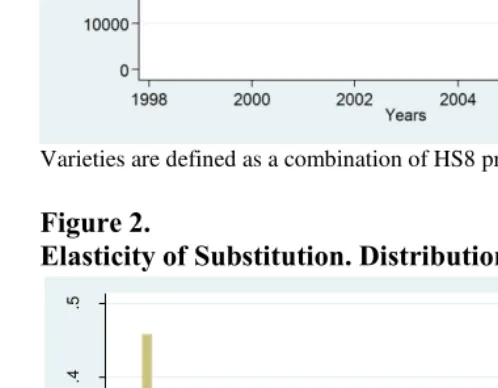
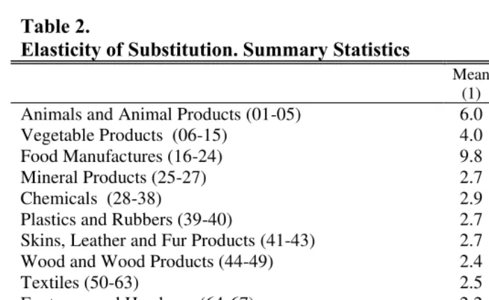
Figure 1 plots the evolution of the total number of imported varieties during the period 1999-2008. There is a significant drop in the number of varieties during the crisis. Table 1 compares varieties in 2000 and 2002. Of the 72,185 varieties that were being imported in 2000, 33,520 varieties stopped being imported between 2000 and 2002 (column 3). During the same period, 13,000 new varieties entered the market (column 4), for a net decline of 20,520 varieties (column 5) or 28.4 percent. The largest declines occur for Animal Products (50 percent), Footwear (49 percent), Textiles (43 percent), Leather and Fur Products (38 percent), and Stone and Glass Products (37 percent). The largest product groups in terms of number of varieties are Metals and Metal Products, Chemicals, and Machinery, which account for 56 percent of the number of varieties imported in 2000 and 46 percent of the decline in the number of imported varieties between 2000 and 2002.

(12)

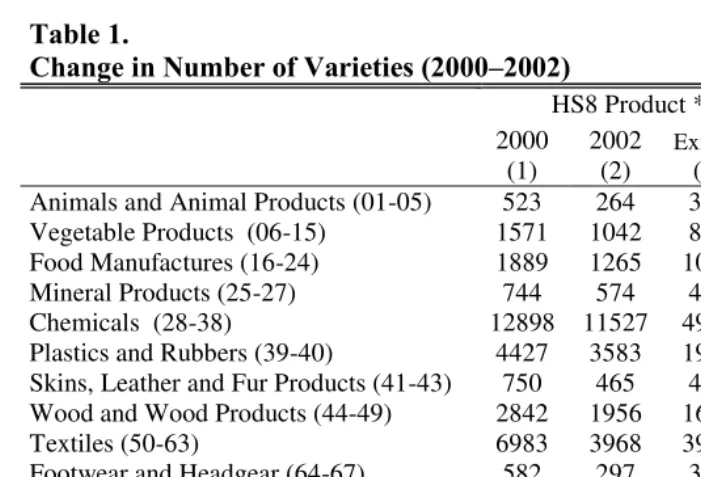
We estimate equation (14) separately for each 2-digit product, for a total of 96 different elasticities of substitution.10_{Figure 2 illustrates the distribution of}

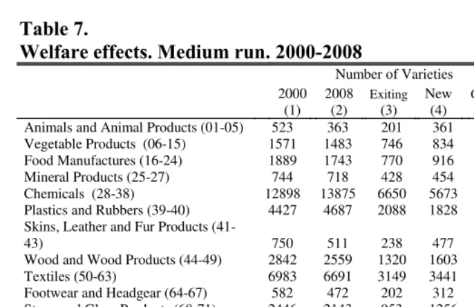
the estimates, and Table 2 shows descriptive statistics by broad groups of products. All elasticities are positive and 90 out of 96 coefficients are statistically significant at the 1 percent level. The majority of the estimates of the elasticity of substitution lies between 1 and 5. The product groups with highest substitution are Food Manufactures, Animal Products, and Vegetable Products, with average estimates of 9.8, 6 and 4. Groups with low estimated elasticity of substitution are Stone and Glass Products, Machinery and Electrical Machinery, and Transportation Equipment. The average of the 96 products is 3.3 and the median is 2.3. These numbers are in line with results in Broda and Weinstein (2006), who estimate a median elasticity of substitution of 2.2 for 3-digit products of the SITC classification.11

Table 3 displays the elasticity of substitution of the 10 products with the largest participation in total imports at 2-digit product level; they are mostly Mineral Products (lines 25, 26 and 27) and Chemicals and Allied Industries (lines 28, 29 y 31). The product with the highest elasticity of substitution is “Fertilizers” (line 31), and the one with the lowest elasticity of substitution is “Electrical Machinery and Equip. and Parts” (line 85); the average estimates are 3.8 and 1.7, respectively. The estimates of the elasticity for the 10 most important products are lower than the average of the 96 products (excepting line 31 and 27), so we can anticipate that a higher participation in the market would make the substitution of varieties more difficult.

Table 4 shows the elasticity of substitution of the products with the highest average price (estimated using unit values). The product “Tobacco and Manuf. Tobacco Substitutes” (Line 24) presents the highest elasticity, with an average estimate of 30.9. This value is 30 times greater than the elasticity of substitution of “Silk, Inc. Yarns and Woven Fabrics Thereof” (line 50), which has the lowest estimated value. The majority of the estimates of sigma in Table

10_{The estimated elasticities of substitution indicate the degree of substitutability of imported}

varieties. They cannot be readily extrapolated to domestic consumption, as the elasticities depend on the degree of heterogeneity across products, which in turn might be different when considering foreign and domestic varieties.

11_{Broda and Weinstein estimate elasticities of substitution at the 3 digit level of the SITC}

(13)

4 are lower than 2, so the products with higher price are more difficult to substitute.

The elasticity of substitution is expected to be lower for homogeneous products or, put in other words, products with a higher degree of heterogeneity are poorer substitutes for each other. We find that indeed our estimates of the elasticity of substitution are lower for more heterogeneous products, proxing for heterogeneity with price dispersion at the product level. More details are provided in the appendix.

III.3. Estimation of the Variety Welfare Effects

We now turn to the estimation of the welfare effects. As discussed in Section 2, variety welfare effects do not depend on the change in the raw number of varieties but rather on their share in 2-digit product expenditure, as defined in equations (7) and (8). Table 5 shows the average share of varieties available in 2 digit-product expenditure before the crisis and after the crisis for each broad product group. A low is associated with a high welfare loss, since it indicates that the participation of exiting varieties in product expenditure was high. A high , on the other hand, indicates that new varieties (which drive welfare up) have not gained a large market share. Column 3 shows the ratio of the market shares. From column 3, we can expect larger welfare losses in the groups with higher ratios: Animal Products, Mineral Products, Textiles, Wood and Wood Products, Vegetable Products, Food Manufactures, and Leather and Fur Products.

The last row of Table 5 shows that the total (across all products) market share of exiting varieties is 14 percent, and the market share of entering varieties is 10 percent. These results suggest that the substitution towards new varieties is larger than indicated when considering the raw count of exiting and entering varieties in Table 1 (33,520 exiting varieties versus 13,000 entering varieties), but that it is not high enough to fully compensate for the loss of varieties.

(14)

Welfare effects vary largely by product. The biggest effects are observed for groups with high market share ratios: Animal Products (57 percent) and Footwear (26 percent).12_{Other groups with large welfare losses are Leather}

and Fur Products (24 percent) and Transportation Equipment (17 percent), all of which have a relative low elasticity of substitution. On the other end of the spectrum we have four groups with average welfare losses between 0.9 and 2.2 percent: Vegetable Products, Food Manufactures, Plastics and Rubbers, Stone and Glass Products. For the remaining six product groups, average welfare losses range between 4.3 and 8 percent.

The total loss in welfare derived from imported products is obtained by weighting the welfare change in each product by the product participation in total imports, as per equation (11).13_{The resulting welfare loss is 7.1 percent.}

We can also compute the loss in welfare derived from total consumption (including imports and domestic consumption), which is 0.9 percent. Notice that this welfare loss does not consider the net exit of domestic varieties from the market and thus underestimates the total welfare loss. Exit of domestic varieties increases welfare losses, while entry of domestic varieties decreases welfare losses because the new domestic varieties could be good substitutes for imports. Our results should be interpreted as the total welfare loss in consumption due to the change in imported varieties only, keeping domestic varieties fixed.14

In columns 2 to 5 we perform a sensitivity analysis with respect to the elasticity of substitution. Rather than using a different (estimated) elasticity of

12_{These changes should be interpreted as equivalent to an increase in the price index. In the case}

of Animal Products, for example, the welfare loss due to the decrease in the number of varieties is the same welfare loss that would occur if the price index rose by 57 percent.

13_{We use the ratio of the market shares to estimate the welfare effect, so the result is not}

influenced by the difference in the number of varieties of each product. The welfare effect depends on the shares of varieties in expenditures of available varieties, and initially a greater or lesser number of varieties does not determine the share or welfare losses. For example, “Knitted or Crocheted Fabrics” (line 60) has 141 varieties, and the welfare loss associated with this line is about 95 percent. The number of varieties of “Articles of Apparel and Clothing Accessories-not Knitted or Crocheted” (line 61) is half of “Knitted or Crocheted Fabrics”, but the estimated

welfare losses are approximately the same (92 percent).

14_{Notice that the entry of domestic varieties becomes more relevant for the case of}

(15)

substitution for each product, we evaluate the welfare loss using a homogeneous elasticity of substitution for all products (of 1.5, 2, 2.5 and 3 in each column, respectively). Using the homogeneous elasticities of substitution, the resulting welfare losses range from 12.6 to 2.8 percent in total imports, and from 1.5 to 0.3 percent in total consumption. This exercise shows that results are very sensitive to the elasticity of substitution for low values of the parameter, but that the sensitivity declines as the parameter increases. It also highlights the importance of using elasticities that vary by product. Our estimated median elasticity of substitution is 2.3, which, if applied to all products homogeneously, would lead to welfare losses between 3.7 and 5.7 percent (columns 3 and 4). When we use the estimated elasticities that vary by product, we obtain higher welfare losses, of 7.1 percent. This difference would be even larger if we used the estimated mean elasticity of substitution of 3.3, which would result in welfare losses between 2.8 and 3.7 percent (columns 4 and 5).

Figure 1 shows that starting in 2003 there is a gradual recovery in the number of imported varieties. Table 7 compares 2000 and 2008, and in columns (1) and (2) shows that the number of available varieties is virtually identical in both years (72,185 in 2000 versus 72,244 in 2008).

How should we interpret this seeming recovery? There are two main issues to consider. The first issue is substitutability between varieties. Table 7 shows that there is considerable turn-over of varieties between 2000 and 2008 (columns (3) and (4)). In other words, there is a substantial number of varieties that exit in 2000 and do not enter again in 2008. This is consistent with the findings of Burstein, Eichenbaum and Rebelo (2005) and McKenzie and Schargrodsky (2011), who document that, during the Argentine crisis, domestic consumers substituted varieties (imported or domestic) towards lower cost alternatives. The extent to which the new varieties are good substitutes for exiting varieties is in our analysis captured by the ratios of market shares, displayed in column (6) of Table 7. These ratios are smaller than the ratios for 2002-2000, indicating that in the medium-run (2008) consumers have been more successful at substituting towards new varieties than in the short-run (2002). Most remarkably, several of the ratios are smaller than one, which indicates a welfare gain.

(16)

worldwide development of new varieties and to the increase in trade linkages. The study of the welfare effects of this phenomenon is the focus of Broda and Weinstein (2006). Additionally, revisions to the harmonized system of product classification could result in an artificial increase in the number of varieties. From this perspective, even though the number of available varieties in 2008 is slightly higher than in 2000, this difference would be even greater if the crisis had not occurred. An accurate welfare measurement would compare the observed varieties in 2008 with the counterfactual varieties in 2008 in the absence of the crisis.

In column (7) of Table 7, we report welfare comparisons between 2000 and 2008. As discussed above, this comparison does not contemplate the increasing trend in the number of varieties, and thus underestimates the (negative) medium-run welfare effects of the crisis. As expected, the negative welfare effects are higher for product groups with high market share ratios: Leather and Fur Products (welfare loss of 30 percent), Animals and Animal Products (19.5 percent), and Metals (10 percent). On the other hand, there are considerable welfare increases in Mineral Products (20 percent) and Stone and Glass Products (10 percent). Other product groups with welfare increases are Vegetable Products, Chemicals, and Wood and Wood Products, all between 1.2 and 2.1 percent. The aggregate welfare loss in the consumption of imports is 4.2 percent, and the welfare loss including domestic consumption is 0.5 percent.

III.3. Additional Results

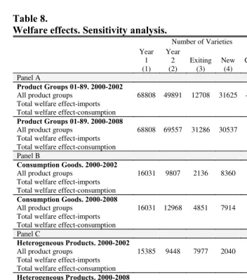
In this section we extend the welfare analysis to consider additional results when we either focus on or exclude particular groups of products. We start by noticing that in Table 7 the largest medium-run welfare losses occur within the product group “Miscellaneous”. In Table 8, panel A, we report welfare results excluding the miscellaneous product group. As expected the medium-run welfare loss is lower when we exclude this product group: 3.1 percent (Table 8) versus 4.2 percent (Table 7).

(17)

are classified as final consumption by the Classification by Broad Economic Categories (BEC, Revision 3).15_{Table 8, panel B presents, as a sensitivity}

analysis, welfare effects derived from imported varieties that are defined as final consumption. The short-run aggregate loss is virtually the same when considering consumption goods only: 6.5 percent (Table 8, Panel B) versus 6.3 percent (Table 8, Panel A, including all goods), which suggests that consumption goods are equally difficult to substitute. In the medium run, however, the welfare losses are larger when we consider consumption goods only (4 percent and 3.1 percent).

Finally, larger welfare losses are expected to be observed within heterogeneous products than within products that are more homogeneous and thus present more possibilities for substitution. In Table 8, panels C and D, we exclude homogeneous products from the analysis. Our definition of homogeneous products is the following. First, for each product, we compute the price dispersion across varieties. Second, we define a product as homogeneous if the variance of the unit values is among the lowest 25th

percentile (panel C) or 10th_{percentile (panel D) across products. As expected,}

welfare losses are larger when we only consider heterogeneous products. The difference is larger in the short run, as possibilities of substitution are more limited.

IV. Conclusion

In this paper we have estimated the welfare loss of Argentine consumers due to the decrease in the number of imported varieties between 2000 and 2002, a period in which the country was hit by a large economic crisis. The estimates show welfare losses between 1 and 57 percent across different product groups, and an aggregate welfare loss in total consumption of imports of 7.1 percent. Medium-run analysis shows that even though the total number of varieties recovers by 2008, important welfare losses still persist during that year for several product groups, leading to an aggregate welfare loss of 4.2 percent.

15_{Gopinath and Neiman (2014) study the decrease in imports of intermediate inputs during the}

(18)

References

Brambilla, I., A. Khandelwal and P. Schott (2010), “China’s Experience under the Multifiber Arrangement and the Agreement on Textile and Clothing,” in Feenstra, R. and S.J. Wei eds., China’s Growing Role in World Trade, University of Chicago Press for the NBER

Broda, C. and D.Weinstein (2006), “Globalization and the Gains from Variety,” Quarterly Journal of Economics, 121(2), pp. 541–585.

Burstein, A., M. Eichenbaum, and S. Rebelo (2005), “Large Devaluations and the Real Exchange Rate,” Journal of Political Economy, 113 (4), pp. 742–784.

Diewert, W. E. (1976), “Exact and Superlative Index Numbers,” Journal of Econometrics, 4, pp. 115–145.

Feenstra, R. (1994), “New Product Varieties and the Measurement of International Prices,” American Economic Review, 84, pp. 157–177.

Gopinath, G., and B. Neiman. (2014). “Trade Adjustment and Productivity in Large Crises,” American Economic Review, 104(3), pp.793-831.

Helpman, E., M. Melitz, and S. Yeaple (2004), “Export Versus FDI with Heterogeneous Firms,” American Economic Review, 94(1), pp. 300-316.

Khandelwal, A. (2010), “The Long and Short (of) Quality Ladders,” Review of Economic Studies, 77(4), pp. 1450-1476.

Krugman, P. (1979), “Increasing returns, monopolistic competition, and international trade,” Journal of International Economics, 9(4), pp. 469-479.

Krugman, P. (1980), “Scale Economies, Product Differentiation, and the Pattern of Trade,” American Economic Review, 70, pp. 950-959.

McKenzie, D. and E. Schargrodsky (2011), “Buying Less, but Shopping More: The Use of Non-Market Labor during a Crisis”, Economía, LACEA, 11(2), pp.

1-43.

(19)

Mohler, L. and M. Seitz (2012), “The Gains from Variety in the European Union,” Review of World Economics, 148(3), pp. 475-500

Sato, K. (1976), “The Ideal Log-Change Index Number,” Review of Economics and Statistics, 63, pp. 223–228.

(20)

[image:20.595.53.304.116.318.2]

Figure 1.

Number of Available Varieties

Varieties are defined as a combination of HS8 product line and country of origin.

Figure 2.

Elasticity of Substitution. Distribution of Estimates

Graph shows the distribution of the estimates of the elasticity of substitution ( ) at the 2-digit level. There is a total of 96 estimates.

0

.1

.2

.3

.4

.5

D

e

n

s

it

y

0 5 10 15 20 25 30

[image:20.595.49.298.352.546.2]

(21)

[image:21.595.54.405.132.371.2]

Table 1.

Change in Number of Varieties (2000–2002)

HS8 Product * Source Country 2000

(1) 2002 (2)

Exiting

(3)

New

(4)

Change

(5)

Animals and Animal Products (01-05) 523 264 358 99 -259

Vegetable Products (06-15) 1571 1042 832 303 -529

Food Manufactures (16-24) 1889 1265 1023 399 -624

Mineral Products (25-27) 744 574 456 286 -170

Chemicals (28-38) 12898 11527 4939 3568 -1371

Plastics and Rubbers (39-40) 4427 3583 1983 1139 -844

Skins, Leather and Fur Products (41-43) 750 465 450 165 -285

Wood and Wood Products (44-49) 2842 1956 1641 755 -886

Textiles (50-63) 6983 3968 3965 950 -3015

Footwear and Headgear (64-67) 582 297 335 50 -285

Stone and Glass Products (68-71) 2446 1534 1276 364 -912

Metals (72-83) 17992 12813 7637 2458 -5179

Machinery and Electrical Machinery (84-85) 9589 6711 4197 1319 -2878

Transportation Equipment (86-89) 5572 3892 2533 853 -1680

Miscellaneous (90-97) 3377 1774 1895 292 -1603

All product groups 72185 51665 33520 13000 -20520

(22)

[image:22.595.54.405.144.359.2]

Table 2.

Elasticity of Substitution. Summary Statistics

Mean (1) Median (2) Min (3) Max (4)

Animals and Animal Products (01-05) 6.0 7.0 1.4 9.9

Vegetable Products (06-15) 4.0 4.0 2.2 5.8

Food Manufactures (16-24) 9.8 7.7 3.8 30.9

Mineral Products (25-27) 2.7 2.3 2.3 3.4

Chemicals (28-38) 2.9 2.7 1.9 4.3

Plastics and Rubbers (39-40) 2.7 1.7 2.6 2.9

Skins, Leather and Fur Products (41-43) 2.7 2.0 1.2 5.1

Wood and Wood Products (44-49) 2.4 2.4 1.5 4.7

Textiles (50-63) 2.5 1.5 1.0 3.9

Footwear and Headgear (64-67) 2.2 1.8 1.1 4.8

Stone and Glass Products (68-71) 1.7 2.1 1.1 2.0

Metals (72-83) 2.1 1.7 1.5 2.9

Machinery and Electrical Machinery (84-85) 1.7 1.6 1.7 1.7

Transportation Equipment (86-89) 1.8 1.5 1.1 2.7

Miscellaneous (90-97) 1.6 2.3 1.3 2.0

All product groups 3.3 2.3 1.0 30.9

(23)

[image:23.595.54.406.140.312.2]

Table 3.

Elasticity of Substitution of the 10 products with largest market share, 2000

HS2 Description Market Share

26 Ores Slag and Ash 24.6% 2.3

27 Mineral Fuels, Oils, Waxes and Bituminous Sub 16.6% 3.4

31 Fertilizers 5.3% 3.8

25 Salt, Sulphur, Earth and Stone, Lime and Cement 4.9% 2.3

85

Electrical Machinery and Equip. and Parts,

Telecommunications Equip., Sound Recorders, Television

Recorders 4.8% 1.7

28 Inorganic Chemicals, Org/Inorg Compounds Of Precious Metals, Isotopes 4.5% 2.3

29 Organic Chemicals 4.4% 2.2

48 Paper and Paperboard, Articles of Paper Pulp 3.8% 2.7

39 Plastics and Articles Thereof 3.4% 2.9

72 Iron and Steel 2.8% 2.6

[image:23.595.56.406.363.547.2]

Table shows the estimates elasticity of substitution ( ) at the 2-digit level of Harmonized System.

Table 4.

Elasticity of Substitution of the 10 products with highest price, 2000

HS2 Description Average Price

71 Pearls, Stones, Prec. Metals, Imitation Jewelry, Coins 8.12 1.15

97 Works of Art, Collectors' Pieces, Antiques 6.37 1.25

85 Electrical Machinery and Equip. and Parts, Telecommunications Equip., Sound Recorders,

Television Recorders 6.2 1.67

29 Organic Chemicals 5.93 2.18

24 Tobacco and Manuf. Tobacco Substitutes 5.67 30.89

91 Clocks and Watches and Parts Thereof 5.43 1.25

88 Aircraft, Spacecraft, and Parts Thereof 5.43 1.13

90 Optical, Photographic, Cinematographic, Measuring, Checking, Precision, Medical or Surgical Instruments

and Accessories 5.06 1.36

30 Pharmaceutical Products 4.8 2.61

50 Silk, Inc. Yarns and Woven Fabrics Thereof 4.58 1.04

(24)

Table 5.

Share of varieties available in both periods (2000–2002)

(1) (2) / (3)

Animals and Animal Products (01-05) 0.73 0.92 1.30

Vegetable Products (06-15) 0.84 0.91 1.08

Food Manufactures (16-24) 0.87 0.93 1.08

Mineral Products (25-27) 0.68 0.76 1.14

Chemicals (28-38) 0.87 0.91 1.05

Plastics and Rubbers (39-40) 0.89 0.91 1.03

Skins, Leather and Fur Products (41-43) 0.92 0.97 1.10

Wood and Wood Products (44-49) 0.60 0.65 1.09

Textiles (50-63) 0.85 0.94 1.13

Footwear and Headgear (64-67) 0.94 0.97 1.03

Stone and Glass Products (68-71) 0.84 0.84 1.00

Metals (72-83) 0.91 0.94 1.04

Machinery and Electrical Machinery (84-85) 0.88 0.92 1.04

Transportation Equipment (86-89) 0.82 0.86 1.06

Miscellaneous (90-97) 0.89 0.94 1.07

All product groups 0.86 0.90 1.06

(25)

[image:25.595.56.393.134.347.2]

Table 6.

Welfare effects. Short run. 2000-2002

= 1.5 = 2 = 2.5 = 3

(1) (2) (3) (4) (5)

Animals and Animal Products (01-05) -0.569 -0.722 -0.297 -0.186 -0.135 Vegetable Products (06-15) -0.022 -0.19 -0.084 -0.054 -0.039 Food Manufactures (16-24) -0.011 -0.167 -0.077 -0.05 -0.037 Mineral Products (25-27) -0.062 -0.308 -0.139 -0.09 -0.066 Chemicals (28-38) -0.043 -0.112 -0.054 -0.035 -0.026 Plastics and Rubbers (39-40) -0.015 -0.054 -0.027 -0.018 -0.013

Skins, Leather and Fur Products (41-43) -0.241 -0.264 -0.1 -0.061 -0.044

Wood and Wood Products (44-49) -0.062 -0.194 -0.092 -0.06 -0.045 Textiles (50-63) -0.084 -0.314 -0.13 -0.082 -0.06 Footwear and Headgear (64-67) -0.256 -0.062 -0.03 -0.02 -0.015 Stone and Glass Products (68-71) 0.009 0.002 0.002 0.001 0.001 Metals (72-83) -0.049 -0.074 -0.036 -0.024 -0.018

Machinery and Electrical Machinery (84-85) -0.055 -0.075 -0.037 -0.024 -0.018 Transportation Equipment (86-89) -0.168 -0.117 -0.056 -0.037 -0.028 Miscellaneous (90-97) -0.248 -0.158 -0.068 -0.043 -0.032

(26)

[image:26.595.55.398.142.364.2]

Table 7.

Welfare effects. Medium run. 2000-2008

Varieties are defined as an HS8 product-country of origin combination. Table shows number of varieties in 2000 (column 1), in 2008 (column 2), varieties that exited between 2000 and 2008 (column 3), new varieties incorporated between 2000 and 2008 (column 4), and the net change in the number of varieties (column 5). Column (6) shows the market share ratios. Column (7) shows the welfare effects based on the estimated elasticity of substitution that varies by 2-digit product.

Number of Varieties _λ j2008/

λj2000 (6)

Welfare effect

(7) 2000

(1) 2008 (2) Exiting(3) New (4) Change(5)

Animals and Animal Products (01-05) 523 363 201 361 -160 1.20 -0.195 Vegetable Products (06-15) 1571 1483 746 834 -88 0.96 0.021 Food Manufactures (16-24) 1889 1743 770 916 -146 1.04 -0.005 Mineral Products (25-27) 744 718 428 454 -26 0.74 0.201 Chemicals (28-38) 12898 13875 6650 5673 977 0.98 0.017 Plastics and Rubbers (39-40) 4427 4687 2088 1828 260 1.05 -0.026 Skins, Leather and Fur Products

(41-43) 750 511 238 477 -239 1.10 -0.298

Wood and Wood Products (44-49) 2842 2559 1320 1603 -283 0.98 0.012

Textiles (50-63) 6983 6691 3149 3441 -292 1.02 -0.012

Footwear and Headgear (64-67) 582 472 202 312 -110 1.06 -0.018 Stone and Glass Products (68-71) 2446 2143 953 1256 -303 0.95 0.099 Metals (72-83) 17992 18774 7306 6524 782 1.06 -0.102 Machinery and Electrical Machinery

(84-85) 9589 9683 4690 4596 94 1.02 -0.029

Transportation Equipment (86-89) 5572 5855 2545 2262 283 1.02 -0.048 Miscellaneous (90-97) 3377 2687 897 1587 -690 1.11 -0.319

All product groups 72185 72244 32183 32124 59 1.02

Total welfare effect-imports -0.042

(27)

[image:27.595.51.403.123.521.2]

Table 8.

Welfare effects. Sensitivity analysis.

Panel A: product group 91-97 is excluded from the welfare computations. Panel B: only consumption goods are included in the welfare computations. Imported varieties classified as final consumption by BEC, Rev. 3. Panels C and D: homogeneous products are excluded from the welfare analysis. Homogeneous products are defined as those in the lowest 25th_{(Panel C)}

and 10th_{(Panel D) percentile of variance in unit values computed across varieties.}

Number of Varieties

λj2/λj1 (6) Welfare effect (7) Year 1 (1) Year 2 (2) Exiting (3) New (4) Change (5) Panel A

Product Groups 01-89. 2000-2002

All product groups 68808 49891 12708 31625 -18917 1.057

Total welfare effect-consumption -0.008

Product Groups 01-89. 2000-2008

All product groups 68808 69557 31286 30537 749 1.018

Panel B

Consumption Goods. 2000-2002

Panel C

Heterogeneous Products. 2000-2002

Panel D

(28)

Appendix A. Elasticity of substitution

In this section we test whether the elasticity of substitution decreases with the degree of product heterogeneity. We use price dispersion as a proxy for product heterogeneity and run regressions of the estimated elasticity on indicator variables that are equal to one if the price dispersion of a given product is above the 25th, 50th, or 75th percentile, in three different specifications.

Results are displayed in Table A1. Coefficients are negative and statistically significant. We find that indeed the elasticity of substitution is lower for more heterogeneous products.

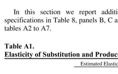
Appendix B. Additional welfare results

[image:28.595.60.298.389.539.2]

In this section we report additional results that correspond to the specifications in Table 8, panels B, C and D, by product groups. Results are in tables A2 to A7.

Table A1.

Elasticity of Substitution and Product Heterogeneity

Standard errors in parentheses. *** p<0.01, ** p<0.05, * p<0.1. Dependent variable: estimated elasticity of substitution. Regressor is a dummy indicating whether price dispersion at the 2-digit level is below the 25th, 50th, and 75th percentile

Estimated Elasticity of Substitution

Price Dispersion -4.027*** . .

Below 25th Percentile (0.719)

Price Dispersion . -2.536*** .

Price Dispersion . . -1.604*

Observations 96 96 96

(29)

[image:29.595.51.403.130.301.2]

Table A2.

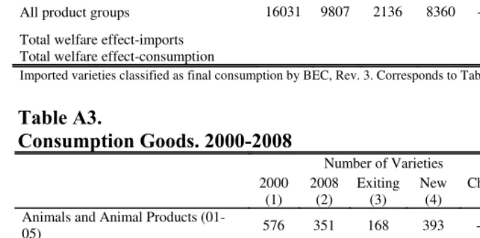
Table A3.

Number of Varieties

λj2002/λj2000 (6) Welfare effect (7) 2000 (1) 2002 (2) Exiting (3) New (4) Change (5)

Animals and Animal Products (01-05) 576 274 85 387 -302 1.189 -0.04 Vegetable Products (06-15) 1341 833 244 752 -508 1.093 -0.025 Food Manufactures (16-24) 2706 2231 570 1045 -475 1.005 -0.003 Mineral Products (25-27) 857 540 66 383 -317 1.027 -0.092

Chemicals (28-38) 977 576 95 496 -401 1.088 -0.102

Plastics and Rubbers (39-40) 1304 758 176 722 -546 0.997 0.001

Skins, Leather and Fur Products (41-43) 2504 1343 273 1434 -1161 1.099 -0.07 Wood and Wood Products (44-49) 784 360 43 467 -424 1.103 -0.07 Textiles (50-63) 3841 2299 471 2013 -1542 0.988 -0.002 Footwear and Headgear (64-67) 1141 593 113 661 -548 1.101 -0.525

Imported varieties classified as final consumption by BEC, Rev. 3. Corresponds to Table 8, panel B.

Number of Varieties

λj2008/λj2000 (6) Welfare effect (7) 2000 (1) 2008 (2) Exiting (3) New (4) Change (5) Animals and Animal Products

(01-05) 576 351 168 393 -225 1.240 -0.048

Vegetable Products (06-15) 1341 1204 540 677 -137 0.988 0.010 Food Manufactures (16-24) 2706 2667 978 1017 -39 0.997 0.004 Mineral Products (25-27) 857 672 182 367 -185 1.037 -0.151

Chemicals (28-38) 977 768 232 441 -209 1.037 -0.020

Plastics and Rubbers (39-40) 1304 1296 637 645 -8 1.098 -0.063

Skins, Leather and Fur Products (41-43) 2504 2273 979 1210 -231 1.016 -0.006 Wood and Wood Products (44-49) 784 489 132 427 -295 1.014 -0.008

Textiles (50-63) 3841 2500 772 2113 -1341 1.544 0.127

Footwear and Headgear (64-67) 1141 748 231 624 -393 1.692 -0.640

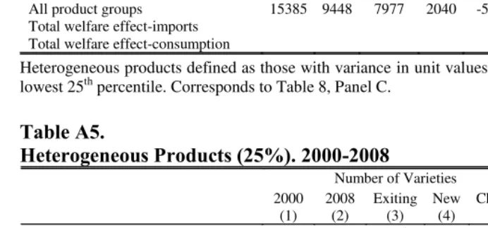
[image:29.595.56.400.345.516.2]

(30)

[image:30.595.55.400.145.316.2]

Table A4.

Heterogeneous Products (25%). 2000-2002

Heterogeneous products defined as those with variance in unit values across varieties above the lowest 25th_{percentile. Corresponds to Table 8, Panel C.}

Table A5.

Heterogeneous products defined as those with variance in unit values across varieties above the lowest 25th_{percentile. Corresponds to Table 8, Panel C.}

Number of Varieties

λj2002/λj2000 (6)

Welfare effect

(7) 2000

(1) 2002 (2) Exiting (3) New (4) Change (5) Animals and Animal Products

(01-05) 320 165 215 60 -155 1.364 -0.066

Vegetable Products (06-15) 1069 668 599 198 -401 1.125 -0.033

Food Manufactures (16-24) 2606 2155 1001 550 -451 1.004 -0.003

Mineral Products (25-27) 857 540 383 66 -317 1.027 -0.092

Chemicals (28-38) 972 575 492 95 -397 1.055 -0.102

Skins, Leather and Fur Products (41-43) 2503 1342 1434 273 -1161 1.147 -0.170

Wood and Wood Products (44-49) 784 360 467 43 -424 1.120 -0.199

Textiles (50-63) 3837 2297 2009 469 -1540 0.987 0.006

Number of Varieties

λj2008/λj2000 (6) Welfare effect (7) 2000 (1) 2008 (2) Exiting (3) New (4) Change (5)

Animals and Animal Products (01-05) 320 222 216 118 -98 1.399 -0.068

Vegetable Products (06-15) 1069 977 527 435 -92 0.996 0.011

Food Manufactures (16-24) 2606 2534 979 907 -72 0.991 0.005

Chemicals (28-38) 972 766 436 230 -206 1.036 -0.018

Textiles (50-63) 3837 2471 2110 744 -1366 1.550 0.125

[image:30.595.55.401.377.538.2]

(31)

[image:31.595.56.402.143.306.2]

Table A6.

Heterogeneous products defined as those with variance in unit values across varieties above the lowest 10th_{percentile. Corresponds to Table 8, Panel D.}

Table A7.

Heterogeneous products defined as those with variance in unit values across varieties above the lowest 10th_{percentile. Corresponds to Table 8, Panel D.}

Number of Varieties

λj2002/λj2000 (6)

Welfare effect

(7) 2000

(1) 2002 (2) Exiting (3) New (4) Change (5)

Animals and Animal Products (01-05) 106 65 74 33 -41 0.648 -0.119

Vegetable Products (06-15) 370 231 191 52 -139 1.066 -0.034

Food Manufactures (16-24) 2276 1916 850 490 -360 1.011 -0.005

Chemicals (28-38) 837 476 436 75 -361 1.018 -0.042

Textiles (50-63) 3683 2167 1936 420 -1516 0.975 0.017

Number of Varieties

λj2008/λj2000 (6)