1Full Time Co-Chair Professor School of Computer Science, UNLP. ldgiusti@lidi.info.unlp.edu.ar. 2Full Time Co-Chair Professor School of Computer Science, UNLP. francoch@lidi.info.unlp.edu.ar. 3Full Time Chair Professor School of Computer Science, UNLP. mnaiouf@lidi.info.unlp.edu.ar.
4CONICET Senior Researcher. Full Time Chair Professor School of Computer Science, UNLP. degiusti@lidi.info.unlp.edu.ar.
Robustness Analysis for the Method of Assignment MATEHa
*Laura De Giusti1, Franco Chichizola2, Marcelo Naiouf3, Armando De Giusti4
Instituto de Investigación en Informática (III-LIDI) – Facultad de Informática – UNLP
ABSTRACT
The TTIGHa model has been developed to model and predict the performance of parallel applications run over heterogeneous architectures.
In addition, the task assignment algorithm was implemented to MATEHa processors based on the TTIGHa model.
This paper analyzes the assignment algorithm robustness before different variations which the model parameters may undergo (basically, communication and processing times).
Keywords: Parallel Systems. Cluster and Multi-cluster Architectures. Performance prediction models. Tasks to processors mapping. Heterogeneous Processors. Robustness.
1.INTRODUCTION
In Computer Science, models are used to describe real entities such as the processing architectures and to obtain an ―abstract‖ or simplified version of the physical machine, capturing crucial characteristics and disregarding minor details of the implementation [1]. A model does not necessarily represent a given real computer, but allows studying classes of problems over classes of architectures represented by their essential components. In this way, a real application can be studied over the architecture model, allowing us to get a significant description of the algorithm, draw a detailed analysis of its execution, and even predict the performance [2].
In the case of parallel systems, the most currently used architectures – due to their cost/performance relation - are clusters and multiclusters; for this reason, it is really important to develop a model that fits the characteristics of these platforms. An essential element to be considered is the potential heterogeneity of processors and communications among them, which adds complexity to the modeling [3][4].
When developing a model for this type of systems, we aim at:
▪Minimizing the conceptual gap between the model and real physical architecture.
▪Simplicity of use.
▪Possibility of determining the correction of an algorithm over the model, and whether this determination is valid independently of the real physical architecture.
▪Capacity for predicting performance.
In these requirements, it is clear that the central objective of parallel computing models is to achieve a performance prediction that fits the real performance of the used multiprocessor architecture.
At present, there exist different graph-based models to characterize the behavior of parallel applications in distributed architectures [5][6]. Among these models, we can mention TIG (Task Interaction Graph), TPG (Task Precedence Graph), and TTIG (Task Temporal Interaction Graph) [7].
But these models suppose an homogeneous supporting architecture, and it is not the general case with clusters and multiclusters. The TTIGHa model consider heterogeneity of processors and communication network [8].
Once the graph modeling the application has been defined, the "mapping" problem is solved by an algorithm that establishes an automatic mechanism to carry out the task-to-processor assignment, searching for the optimization of some running parameter (usually, time) [9][10][11]. This is a NP-complete problem, due to the number of factors to be considered, which affects the application running time, directly or indirectly. In general, static mapping algorithms can be of two types:
▪ Optimal: all the possible ways to assign the tasks onto the processors are evaluated. This kind of solutions is feasible only when the quantity of configurations is very small. Otherwise, we can not obtain the optimal solution because of the combinatorial explosion for the number of possible solutions.
▪ Heurístic: they are based in approximation techniques that use ―realistic‖ assumptions for the algorithm and the parallel system. They produce sub-optimal solutions but with acceptable response times.
Naturally, an important topic is that of robustness of the mapping automatic algorithm that is being developed. A robust solution will allow reducing the error in the task-to-processor assignment due to errors in the application parameters (processing times, communication times) [12][13].
In this work, the robustness of MATEHa (the assignment algorithm developed for the TTIGHa model) is analysed. For this, different experimental tests wer carried out considering the algorithm’s behaviour when the input parameters (execution and communication times between tasks) are not known exactly.
2. TTIGHa MODEL
The TTIGHa model is based on the construction of a graph G(V,E) to represent the application to be modeled [8]. For the construction of such graph, we use, apart from the application information, parameters allowing the characterization of the architecture (Tp,Tc), where Tp is the set of processors and Tc represents the set of communication classes. The elements making up the graph are:
▪ V, is the set of nodes. Each of them represents a task Ti of the parallel program.
▪ E, is the set of edges representing the communication among the graph nodes.
2.1.Details of the Model Parameters
Tp involves the set of processors. As the architecture can be heterogeneous, we have a set of different types of processors, and each element of the Tp set should specify to which type it belongs.
Tc represents the set of communication classes. Each class of the set is characterized by the startup time and the bit transmission time.
In the first parameter of graph (V), each node Ni
represents a task Ti. In Ni, the running time
corresponding to Ti in each processor type is stored:
Wi(s) is the time necessary to run task Ti in processor
s.
In the second parameter of graph (E), the edges represent each communication existing between each task pair. In this set, an edge A between two tasks Ti and Tj keeps a matrix C of dimension [mxm]
(m: quantity of the architecture processors), where Cij(s,d) is the communication time between task Ti
located in processor s and task Tj located in
processor d. It is important to notice that the communication cost depends on the processors being communicated because the interconnection network is considered as heterogeneous. In addition, the edge A keeps the ―degree of concurrence‖ between task Ti and task Tj.
The ―degree of concurrence‖ (DoC) is a matrix Hij
of dimension [mxm], where Hij(s,d) represents the
degree of concurrence between task Ti in processor s
and task Tj in processor d. This index is normalized
between 0 and 1. For two tasks, Ti and Tj, being
communicated from Ti to Tj, DoC is defined as the
maximum percentage of Tj computing time that can
be performed in parallel with Ti, taking into account
their mutual dependences arising from the communications existing between both tasks, and disregarding the communication cost associated to them (this generates a value independent of the data to be transmitted). Eq. (1) shows the degree of concurrence (DoC) between tasks Ti and Tj being
executed in processor s and d respectively.
) 1 ( )
( ) , ( ) , (
d W
T T TP d s H
j j i sd
ij
where TPsd(Ti,Tj) is the maximum joint running time
between both tasks in the corresponding processors.
3.MATEHa ALGORITHM
MATEHa is a static prediction algorithm that allows determining the assignment of tasks to the processors of the architecture to be used, aiming at the minimization of the application running time on such architecture. MATEHa considers an architecture with a bounded number of processors, which can be heterogeneous in terms of their computing power and of the interconnection network [8].
MATEHa strategy consists in determining, for each of the tasks of graph G made up by the TTIGHa model, to which processor it should be assigned in order to achieve the highest performance of the application in the used architecture. Such assignment makes use of the values generated in the graph construction: a task computing time in each processor, communication time with its adjacent (which also depends on where the tasks have been assigned) and, finally, the degree of parallelism among tasks. This last value is useful for assigning to the same processor those tasks with lesser degree of parallelism, and to different processors, those with higher degree of parallelism.
assignment is defined with certain priority.
In second place, for each level n of the graph (beginning by level 0), the assignment of all of its tasks to the processors is carried out. For this, in each step, the task not yet assigned and belonging to level n is chosen, which generates the maximum gain by assigning such task to a processor. The gain of a task Ti is obtained as the difference between the
cost of running Tiin the ―worst processor‖ and the
execution of Tiin the ―best processor‖ (this does not
imply that the best/worst processor is the fastest/slowest, respectively).
In order to compute the cost c of running task Ti in a
processor p, two actions are computed. The first add to the time accumulated in p (this time is the sum of the running times of the tasks already assigned to it) the time required to run Ti in p. In the second, for
each task Ta adjacent to Ti, which has already been
assigned to a processor q (different to p), the communication time between Ti and Ta in both
directions (Ci,a(p,q) and Ca,i(q,p)) and the time in
which Ti and Ta cannot be run jointly - i.e., the
percentage in which they are not concurrently run (1 – Hia(p,q)) multiplied by the time of running Ta in q
- are accumulated to cost c.
4.MATEHa ALGORITHM ROBUSTNESS
An algorithm’s robustness is related to the variation sensitivity in estimating the model input parameters. For the used model, the parameters that can be inexact at the moment of computing the assignment are: each task running time in each different type of processor and communication times on the network used for the same task.
The MATEHa algorithm sensitivity considering the variations of the previously mentioned parameters was experimentally measured. Values near zero mean that the MATEHa algorithm assigns in a proper manner, despite the included variations.
In order to analyze the robustness of the MATEHa algorithm, different experimental tests were carried out. The architecture configuration for the tests and the set of applications to be evaluated were chosen. Then an assignment using the MATEHa algorithm was generated and the robustness of the assignment was tested.
4.1.Choosing the Architecture for the Tests.
The heterogeneous architecture used is made up by two clusters interconnected by a switch. The first (cluster 1) is composed by 20 processors (P IV 2,4Ghz, 1Gb Ram) and the second (cluster 2) by 10 processors, (Celeron, 2 GHz, 128Mb Ram). The connection is made through an Ethernet network of 100 Mbits. This architecture was chosen so that the
clusters making it up are of different characteristics in terms of the processors´ computing power.
For the tests, different subsets of processors of each cluster were chosen, making up four configurations (Cf1 – Cf4): Cf1:4 processors belonging to cluster 1; Cf2: 3 processors belonging to cluster 1 and 1 belonging to cluster 2; Cf3: 2 processors belonging to cluster 1 and 2 processors belonging to cluster 2; Cf4: 1 processor belonging to cluster 1 and 3 processors belonging to cluster 2.
4.2.Choosing the Set of Applications to be Evaluated
A set of applications was chosen, in which each of them varied in terms of: application task quantity, task size, quantity of subtasks making up a task, and communication volume among subtasks. All of these characteristics should be configured for each application. In all the applications, the total computing time exceeds that of communications.
In each of the tests carried out for the different applications, the configuration of the architecture to be used should be first indicated. Once the architecture is chosen, we should specify the different types of processors, the quantity of processors for each of these types, the different types of communication, the startup and transference times for each of these types, and, finally, the communication type used between each pair of processors. Once this information is specified, graph G is created - generated from the TTIGHa model.
4.3.Generating Assignments with MATEHa
For each of the graphs generated in each test explained in point (4.2), the assignment is computed by the MATEHa algorithm. Then, after this assignment, the application is run over the real architecture in order to obtain the response time. As last step, in order to determine the MATEHa algorithm efficiency, the time obtained using the assignment generated by MATEHa is compared to the time obtained by the optimal assignment (that which minimizes the application response time).
In order to compute the optimal assignment, all the possible assignments of each application task to each processor of the architecture should be evaluated. Since this computation is highly costly in time, the chosen configurations have four processors. For the tests described above, in a previous work we show that the difference with the optimal assignment is less than 12% [8]
4.4.Testing the Algorithm Robustness
For each of the applications defined in point (4.2), tests are carried out adding different percentages of variations in the computing and/or communication time. Each considered variation is a random value between 0 and a maximum percentage (different, according to computing or communication). The values for the maximum percentage taken into account are of 0 to 100 % at intervals of 10%. In order to obtain a most significant sample, 10 runs are generated for each of these variations. In each test, the following steps are carried out:
a. For the application to be run, the TTIGHa model is run.
b. The assignment is obtained (by means of the MATEHa mapping algorithm) for that application according to the times indicated in the test.
c. The new computing and/or communication times are computed, adding to them the corresponding variation percentage.
d. With the assignment obtained in (4.4.b) and the new times computed in (4.4.c), the simulation of the application execution is generated in order to obtain the final time.
e. With the times obtained in (4.4.b), the assignment is obtained also using MATEHa, and then the simulation for such assignment is carried out.
f. The final times obtained by simulations of points (4.4.d) and (4.4.e) are compared. The closest such times are, it means that the achieved assignment by the MATEHa algorithm is slightly affected by the variations in the model times.
5.RESULTS
In order to analyze the results obtained, for each of the different variation percentages (0..100%), the following is computed:
▪ Percentage of tests in which there existed an error, i.e., in which the final time obtained in points (4.4.d) and (4.4.e) was different (% Test with Error).
▪ Average error. The error in a test is given by the difference in the times obtained in (4.4.d) and (4.4.e) with respect to the time obtained in (4.4.e) (General Average Error).
▪ Average error of the tests that obtained different results in (4.4.d) and (4.4.e); this value is computed in order to carry out a more detailed analysis of the error influence in the results (Trimmed Average Error).
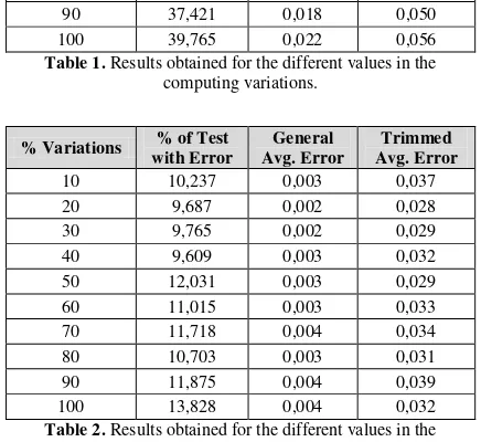
Table 1 shows the results for the tests with variations only for computing times, and Table 2 for
different values only in the communications variations.
% Variations % of Test with Error
General Avg. Error
Trimmed Avg. Error
10 7,968 0,003 0,042
20 11,718 0,003 0,026
30 19,296 0,006 0,034
40 21,640 0,009 0,042
50 27,343 0,012 0,046
60 28,750 0,013 0,047
70 30,078 0,015 0,052
80 36,093 0,017 0,048
90 37,421 0,018 0,050
[image:4.595.309.526.115.315.2]100 39,765 0,022 0,056
Table 1. Results obtained for the different values in the computing variations.
% Variations % of Test with Error
General Avg. Error
Trimmed Avg. Error
10 10,237 0,003 0,037
20 9,687 0,002 0,028
30 9,765 0,002 0,029
40 9,609 0,003 0,032
50 12,031 0,003 0,029
60 11,015 0,003 0,033
70 11,718 0,004 0,034
80 10,703 0,003 0,031
90 11,875 0,004 0,039
100 13,828 0,004 0,032
Table 2. Results obtained for the different values in the communication variations.
The Figure 1 shows the % of Test with Error obtained for the different values in the computing and communication variations. It can be noticed that, when increasing the variation percentage in computing, this generates an increase of the percentage of tests with error; however, this does not happen in the same way as when varying the communication values alone.
0 5 10 15 20 25 30 35 40 45
10 20 30 40 50 60 70 80 90 100
%
o
f
T
e
st
w
it
h
E
rr
o
r
[image:4.595.309.527.218.418.2]% Va ria tion Only Computing va ria tions Only Communica tion Va ria tions
Fig. 1.% of test with error in test with computing and communication variations.
[image:4.595.312.524.546.663.2]0 0,005 0,01 0,015 0,02 0,025
10 20 30 40 50 60 70 80 90 100
G
e
n
e
ra
l
A
v
e
ra
g
e
E
rr
o
r
[image:5.595.312.525.67.413.2]% Va ria tion Only Computing va ria tions Only Communica tion Va ria tions
Fig. 2.General Average Error in test with computing and communication variations.
In them, we can see that, for all the variations, the trimmed error percentage does not exceed the 6%, whereas the general error percentage does not exceed the 2.5%.
0 0,01 0,02 0,03 0,04 0,05 0,06
10 20 30 40 50 60 70 80 90 100
T
ri
m
m
e
d
A
v
e
ra
g
e
E
rr
o
r
[image:5.595.72.283.69.189.2]% Va ria tion Only Computing va ria tions Only Communica tion Va ria tions
Fig. 3.Trimmed Average Error in test with computing and communication variations.
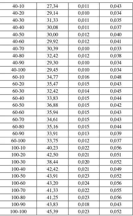
The Table 3 shows some of the results obtained in which different variations both in computing and in communications have been carried out. The complete group of results is in [14]
The Figure 4 show the % Test with Error obtained for some test in which different variations both in computing and in communications have been carried out.
When combining the variations both in the computing times and those of communications, we can notice that, with respect to the percentages of tests in which errors were detected, it keeps the features found when analyzing the variations in the computing, though with a slight increase. This same relation is kept in all the tests carried out, which are presented in more detailed in [14].
% Variations Comp – Comm
% of Test with Error
General Avg. Error
Trimmed Avg. Error
10-10 16,95 0,005 0,032
10-20 17,97 0,006 0,033
10-30 19,77 0,006 0,032
10-40 15,78 0,005 0,036
10-50 16,02 0,006 0,042
10-60 18,28 0,007 0,038
10-70 18,05 0,005 0,031
10-80 18,44 0,005 0,028
10-90 17,89 0,005 0,031
10-100 18,59 0,006 0,036
40-10 27,34 0,011 0,043
40-20 29,14 0,010 0,034
40-30 31,33 0,011 0,035
40-40 30,08 0,011 0,037
40-50 30,00 0,012 0,040
40-60 29,92 0,012 0,041
40-70 30,39 0,010 0,033
40-80 32,42 0,012 0,038
40-90 29,30 0,010 0,034
40-100 29,45 0,010 0,034
60-10 34,77 0,016 0,048
60-20 35,47 0,015 0,043
60-30 32,42 0,014 0,045
60-40 33,83 0,015 0,044
60-50 36,88 0,015 0,042
60-60 35,94 0,015 0,043
60-70 34,61 0,015 0,043
60-80 35,16 0,015 0,044
60-90 33,91 0,013 0,039
60-100 33,75 0,012 0,037
100-10 40,23 0,022 0,056
100-20 42,50 0,021 0,051
100-30 38,44 0,020 0,052
100-40 42,42 0,021 0,049
100-50 43,91 0,023 0,052
100-60 43,20 0,024 0,056
100-70 41,33 0,022 0,055
100-80 41,25 0,023 0,056
100-90 43,83 0,018 0,043
100-100 45,39 0,023 0,052
Table 3. Results obtained for some combinations of values of computing and communications variations.
The Figure 5 and 6 shows the General and Trimmed Average Error respectively obtained in which different variations both in computing and in communications have been carried out.
Like with the percentage of tests with error, when combining the variations both in computing and communications times, we can observe that both the general average error and the trimmed one keep the form found when analyzing only variations in the computation, i.e., they increase as the % in the computing time variation increases. This same relation is kept for the remaining tests, which are not shown.
0 5 10 15 20 25 30 35 40 45 50
10 20 30 40 50 60 70 80 90 100
%
o
f
T
e
st
w
it
h
E
rr
o
r
% Va ria tion in Communica tion 10% 40% 60% 100%
Fig. 4.%Tests with Error obtained for the different values in the communication variations with 10%, 40%, 60% and 100 % of
[image:5.595.71.283.281.400.2] [image:5.595.310.525.614.736.2]0 0,005 0,01 0,015 0,02 0,025 0,03
10 20 30 40 50 60 70 80 90 100
G
e
n
e
ra
l
A
v
e
ra
g
e
E
rr
o
r
[image:6.595.71.284.71.193.2] [image:6.595.71.283.236.360.2]% Va ria tion in Communica tion 10% 40% 60% 100%
Fig. 5.General Average Error obtained for the different values in the communication variations with 10%, 40%, 60% and 100 % of
variation in computing.
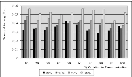
0 0,01 0,02 0,03 0,04 0,05 0,06
10 20 30 40 50 60 70 80 90 100
T
ri
m
m
e
d
A
v
e
ra
g
e
E
rr
o
r
% Va ria tion in Communica tion 10% 40% 60% 100%
Fig. 5.Trimmed Average Error obtained for the different values in the communication variations with 10%, 40%, 60% and 100 %
of variation in computing.
6.ANALYSIS OF RESULTS AND CONCLUSIONS
As regards robustness, we can say that for the tests carried out, in which only a variation in the computation is made, it can be noticed that, by using a variation of up to the 60%, the percentage of tests with error does not exceed the 30%. In the tests carried out only with variations in the communication times, we could see that the error percentage with respect to the optimal mapping does not exceed the 14%, even making variations of the 100%. In addition, the error is practically kept constant.-
Similarly, in the tests in which variations were made both in computing and communication times, we can see that the percentage of tests with error keeps the form found when only varying the computing time, though with a slight, relatively constant increase caused by varying the communication time. In this case, we get a 37% of error when using a variation of the 60% in the computing time.
As regards the trimmed average error, we can see a slight increase as the variation in the computing time increases; however, in no case does it exceed the 6%. Finally, it happens the same in the general average error, without exceeding the 2.5%.
These results allows us to conclude that the MATEHa algorithm presents a high degree of
robustness, since it is able to carry out a good assignment, without the need of using exact parameters in terms of computing and communication times.
7.FUTURE WORK
This study of the MATEHa mapping algorithm with the aim of obtaining a speedup and a reachable load balance optimization will be continued. Particular emphasis will be put in studying the cases in which the multi-cluster involves several communication stages.
Also we’re extending experimental work to check MATEHa results with optimal assignment results for increasing number of processors (8, 12 and 16).
Improvements will be done in the MATEHa algorithm in order to determine the optimal automatic architecture, and from that datum we will try to achieve an allocation that increases the application efficiency without increasing its final time.
8.REFERENCES
[1] Grama A., Gupta A., Karypis G., Kumar V.: An Introduction to Parallel Computing. Design and Analysis of Algorithms. 2nd Edition. Pearson Addison Wesley (2003).
[2] Attiya H., Welch J.: Distributed Computing: Fundamentals, Simulations, and Advanced Topics. 2nd Edition. Wiley-IEEE, New Jersey (2004).
[3] Leopold C.: Parallel and Distributed Computing. A survey of Models, Paradigms, and Approaches. Wiley, New York (2001).
[4] Kalinov A., Klimov S.: Optimal Mapping of a Parallel Application Processes onto Heterogeneous Platform. In: Proceeding of 19th IEEE International Parallel and Distributed Processing Symposium (IPDPS’05). IEEE CS Press (2005).
[5] Roig C., Ripoll A., Senar M.A., Guirado F., Luque E.: Modelling Message-Passing Programas for Static Mapping. In: Euromicro Workshop on Parallel and Distributed Processing (PDP’00), pp. 229--236, IEEE CS Press, USA (1999).
[6] Hwang J.J., Chow Y.C., Anger F.D., Lee C.Y.: Scheduling Precedence Graphs in Systems with Interprocessor Communication Times. SIAM Journal of Computing, 18(2), 244—257 (1989).
[7] Roig C.: Algoritmos de asignación basados en un nuevo modelo de representación de programas paralelos. Tesis Doctoral, Universidad Autónoma de Barcelona (2002).
[8] De Giusti L., Chichizola F., Naiouf M., Ripoll A., De Giusti A.: A Model for the Automatic Mapping
Multicluster Architecture. Journal of Computer Science and Technology 7(1), 39--44 (2007).
[9] Cuenca J., Gimenez D., Martinez J.: Heuristics for Work Distribution of a Homogeneous Parallel Dynamic Programming Scheme on Heterogeneous Systems. In: Proc. of the 3rd International Workshop on Algorithms, Models and Tools for Parallel
Computing on Heterogeneous Networks
(HeteroPar’04). IEEE CS Press (2004).
[10] Cunha J.C., Kacsuk P., Winter S.: Parallel Program development for cluster computing: methodology, tools and integrated environments. Nova Science Pub., New York (2001).
[11] Roig C., Ripoll A., Senar M., Guirado F., Luque E.: Exploiting knowledge of temporal behavior in parallel programs for improving distributed mapping. In: Euro-Par 2000. LNCS, vol. 1900, pp. 262--71. Springer, Heidelberg (2000).
[12] England D., Weissman J., Sadagopan J.: A New Metric for Robustness with Application to Job Scheduling. In: Proceeding of International Symposium on High Performance Distributed Computing 2005 (HPDC-14), pp. 135--143. IEEE Press (2005).
[13] Ali, S., Maciejewski, A.A., Siegel, H.J., Kim, J.-K.: Definition of a robustness metric for resource allocation. In: Proceedings of the 17th IEEE International Parallel and Distributed Processing Symposium (IPDPS’03). IEEE CS Press (2003).
[14] Chichizola F., De Giusti L.: Algoritmo
MATEHa/modelo TTIGHa. Pruebas experimentales
variando parámetros de procesamiento y