Design & implementation of a powered wheelchair control system using EOG signals

Texto completo

(1)MSc. BIOINFORMATICS & BIOSTATISTICS. MASTER’S THESIS. Design & Implementation of a powered wheelchair control system using EOG signals. AUTHOR: Jayro Martı́nez Cerveró RESEARCH SUPERVISOR: Dr. Ujwal Chaudhary ACADEMIC SUPERVISORS:: Dr. Ferran Reverter Comes Dr. Esteban Vegas Lozano. June 2019.

(2) Under Creative Commons License Attribution NonCommercial NoDerivs 3.0 (CC BY-NC-ND 3.0).

(3) Design & Implementation of a powered wheelchair control system using EOG signals Author Jayro Martı́nez Cerveró Research Supervisor Dr. Ujwal Chaudhary Academic Supervisors Dr. Ferran Reverter Comes & Dr. Esteban Vegas Lozano Date 06/2019 MSc. Title Bioinformatics & Biostatistics Thesis Area Machine Learning Manuscript Language English Electrooculography, Human-Computer Interface, Keywords SVM classification Abstract The goal of the project is to design and implement a powered wheelchair control system using electrooculographic signals. The system aims to help people with reduced mobility to control the mentioned wheelchair using eye movements, enabling them to take advantage of the mobility and autonomy advantages that this kind of system could provide to them. One of the crucial component of this system is implementation of the data acquisition and pre-processing as well as the signal feature extraction, signal classification and control system based on that classification. A Support Vector Machines (SVM) based Machine Learning technique was used for classification. These methods were developed and implemented during this proposed work with the aim to enable eye movement based wheelchair control. Title.

(4) Contents 1 Introduction 1.1 Context and Motivations . . . . . . . . . . . 1.1.1 Amyotrophic Lateral Sclerosis (ALS) 1.1.2 Eye movement detection . . . . . . . 1.1.3 Human-Computer Interfaces (HCIs) . 1.1.4 Support Vector Machines (SVMs) . . 1.1.5 Feature extraction . . . . . . . . . . 1.2 Objectives . . . . . . . . . . . . . . . . . . . 1.3 Materials and Methods . . . . . . . . . . . . 1.3.1 Acquisition . . . . . . . . . . . . . . 1.3.2 Signal pre-processing . . . . . . . . . 1.3.3 Feature extraction . . . . . . . . . . 1.3.4 Classification . . . . . . . . . . . . . 1.3.5 Control paradigm & control system . 1.4 Task Planning . . . . . . . . . . . . . . . . . 1.5 Product Summary . . . . . . . . . . . . . . 1.6 Descripton of the Memory . . . . . . . . . . 2 Results. . . . . . . . . . . . . . . . .. . . . . . . . . . . . . . . . .. . . . . . . . . . . . . . . . .. . . . . . . . . . . . . . . . .. . . . . . . . . . . . . . . . .. . . . . . . . . . . . . . . . .. . . . . . . . . . . . . . . . .. . . . . . . . . . . . . . . . .. . . . . . . . . . . . . . . . .. . . . . . . . . . . . . . . . .. . . . . . . . . . . . . . . . .. . . . . . . . . . . . . . . . .. . . . . . . . . . . . . . . . .. . . . . . . . . . . . . . . . .. . . . . . . . . . . . . . . . .. . . . . . . . . . . . . . . . .. . . . . . . . . . . . . . . . .. 2 2 2 2 4 5 7 8 9 9 10 11 12 12 14 15 15 17. 3 Conclusions 23 3.1 Future Work . . . . . . . . . . . . . . . . . . . . . . . . . . . . . . . . . . . 23 4 Glossary. 25. 5 Supplementary Material 27 5.1 Pre-processing function . . . . . . . . . . . . . . . . . . . . . . . . . . . . . 27 5.2 Feature extraction function . . . . . . . . . . . . . . . . . . . . . . . . . . . 28 5.3 Classification function . . . . . . . . . . . . . . . . . . . . . . . . . . . . . 30. iii.

(5) List of Tables 2.1. Minimum, maximum and average accuracies with 5-fold cross-validation. iv. . 21.

(6) List of Figures 1.1 1.2 1.3 1.4 1.5 1.6 1.7 1.8 1.9 1.10 1.11. Waveform of an EOG signal [1] . . . . . . . . . . . . . . . Electrode placement for EOG signal acquisition [2] . . . . Boundary created by a SVM [3] . . . . . . . . . . . . . . . Boundaries created by Polynomial and Gaussian kernels [4] OpenBCI Cyton board . . . . . . . . . . . . . . . . . . . . Control paradigm diagram . . . . . . . . . . . . . . . . . . Task planning for February . . . . . . . . . . . . . . . . . . Task planning for March . . . . . . . . . . . . . . . . . . . Task planning for April . . . . . . . . . . . . . . . . . . . . Task planning for May . . . . . . . . . . . . . . . . . . . . Task planning for June . . . . . . . . . . . . . . . . . . . .. 2.1. EOG vertical and horizontal components before pre-processing. The samples correspond to Left, Up, Left, Left, Left, Down, Right, Up, Left and Right movements . . . . . . . . . . . . . . . . . . . . . . . . . . . . . . . EOG vertical and horizontal components after pre-processing. The samples correspond to Left, Up, Left, Left, Left, Down, Right, Up, Left and Right movements . . . . . . . . . . . . . . . . . . . . . . . . . . . . . . . . . . . Values for horizontal (top) and vertical (bottom) components for Minimum feature. From left to right: Up, Down, Left and Right movements . . . . Values for horizontal (top) and vertical (bottom) components for Maximum feature. From left to right: Up, Down, Left and Right movements . . . . Values for horizontal (top) and vertical (bottom) components for Area Under the Curve feature. From left to right: Up, Down, Left and Right movements . . . . . . . . . . . . . . . . . . . . . . . . . . . . . . . . . . . Values for horizontal (top) and vertical (bottom) components for Derivative Slope feature. From left to right: Up, Down, Left and Right movements .. 2.2. 2.3 2.4 2.5. 2.6. v. . . . . . . . . . . .. . . . . . . . . . . .. . . . . . . . . . . .. . . . . . . . . . . .. . . . . . . . . . . .. . . . . . . . . . . .. . . . . . . . . . . .. . . . . . . . . . . .. . . . . . . . . . . .. 3 4 6 6 10 13 14 14 14 15 15. . 17. . 18 . 18 . 19. . 19 . 20.

(7)

(8) Chapter 1 Introduction 1.1. Context and Motivations. This thesis was proposed by Dr. Ujwal Chaudhary and it has been developed under his supervision at the Neurofeedback and Stimulation department in the Institute of Medical Psychology and Behavioural Neurobiology in Tübingen, Germany. Several conditions could affect human mobility and the capacity to use a conventional wheelchair. These conditions include spinal cord injury, apoplexy, muscular distrophy and Amyotrophic Lateral Sclerosis (ALS), one of the most common of these conditions.. 1.1.1. Amyotrophic Lateral Sclerosis (ALS). Amyotrophic Lateral Sclerosis or ALS is a neurodegenerative disorder. This disorder has a prevalence of 4.8 per 100.000 people and a standarized incidence rate of 1.67 per 100.000 person/year [5]. ALS leads to progressive muscle weakness and the lost of voluntary movements [6]. Usually, the last motor response to be lost in these kind of patients is the eye movements, taking the patient from the condition of Locked-in syndrome (LIS) to Completely Locked-in state (CLIS) [7]. Due to the nature of this neurodegenerative disorder and taking into account that eye movements are the last to be lost in this kind of patients, a Human-Computer Interface (HCI) based on eye movements could be an interesting solution to mantain their movement independence in order to give them the best quality of life.. 1.1.2. Eye movement detection. There are several techniques for measuring or detect the eye movements. In this section we are going to present some of them, as well as their advantages and disadvantages. Electrooculography (EOG) In 1849, Du Bios-Reymond observed there was a relation between electrode potentials from the skin surface and eye movements [8]. The technique of recording these potentials 2.

(9) CHAPTER 1. INTRODUCTION. Figure 1.1: Waveform of an EOG signal [1] is known as Electrooculography (EOG) and was introduced for diagnostic purposes by R. Jung in the 1930s [9]. The potential difference in EOG comes from the large presence of electrically active nerves in the posterior part of the eyeball, where the retina is placed, and the front part, where we can find the cornea [1]. This creates an electrical dipole between the cornea and the retina and its movements generates the potential differences that we can record in an EOG. The voltage values in EOG varies from 50 to 3500 µV with a frequency of 100 Hz. It has a practically linear behaviour for gaze angles of ± 30◦ and it changes approximately 20 µV per degree [10]. A waveform corresponding to up and down movements could be seen in Figure 1.1. For acquiring this signals some electrodes need to be placed near the eyes in contact with the skin. The electrode position should be adequate to capture horizontal and vertical components on the eye movements. An example of the electrode position could be seen in Figure 1.2. In this figure, electrodes B and C are used to calculate the vertical component, electrodes D and E for the horizontal component and electrode A is used to establish the ground or reference for the signal. This technique present some advantages such as not limiting the patients field of view, ease of use and being noninvasive. On the other hand, its disadvantages are the changes on the signal amplitude with the amount of ambient light, the cost of the amplifiers needed for measuring and the contamination of the signal by electrical, electroencephalographic and electromyographic artifacts [9]. This technique is probably the most used in HCI [11][12][13]. Infrared Reflection Oculography (IROG) This technique relies on the fact that the white sclera reflects more light than the pupil and the iris. This fact could be used measuring the amount of light reflected in a certain moment to the sensor. Some of the advantages include a high resolution on small hor-. 3.

(10) CHAPTER 1. INTRODUCTION. Figure 1.2: Electrode placement for EOG signal acquisition [2] izontal movements, a low cost of the recording (except for the equipment) and a stable baseline. This technique present some disadvantages like the obstruction of the subjects view, a very limited angle for vertical recordings and the presence of interferences because of the ambient light. We can see an example of this technique in [14]. Vision-based systems Also known as videooculography systems or Purkinje eye-trackers, these systems mounts a videocamera to track the image of the pupil or the light reflexes generated by the surfaces of the cornea and the lens. Usually these systems use infrared light for illuminating the eye and then process the image by some digital image software. The frame rate depends on the camera used in the system. This technique present some advantages over IROG like its superior linear range. Also these systems are intuitive, easy to handle and could let patients head movements free. Its main disadvantage is the frame rate, being in most cases not enough to record some of the fastest eye movements. In addition, these systems could need to obstruct the view of the subject with the camera and head-mounted systems should be tightly fixed, being uncomfortble to wear [9]. One example of this kind of technique could be seen in [15].. 1.1.3. Human-Computer Interfaces (HCIs). Also known as Human-Machine Interfaces (HMIs) and for some particular cases BrainComputer Interfaces (BCIs), these systems are created to bridge the gaps that exist between humans and machines [16]. The aim of this interfaces is to tranlste the user inputs into computer commands to provide the desired result. These technologies could 4.

(11) CHAPTER 1. INTRODUCTION be applied to a wide range of purposes like moving a computer cursor [17], control a keyboard [18] or a prothesis [19], rehabilitation [20], communication [21] or just like in our case, to control a wheelchair [22][23][24][2]. Depending on the nature of the inputs HCIs could be classified, among others, into voice-based [25], vision-based [26] or, probably the most interesting case, biosignal-based. This last paradigm include input signals as EOG, electromyography (EMG) [27], electroencephalography (EEG) [28] and near-infrared spectroscopy (NIRS) [29]. In case that the signal comes from the brain, like in EEG and NIRS, we are talking about a braincomputer interface, a growing field in the last decades [20].. 1.1.4. Support Vector Machines (SVMs). Despite the fact that some biosignal-based HCIs use other machine learning techniques like artificial neural networks [10][30] or even other statistical techniques [1], most of the HCIs present in the literature use the machine learning technique called Support Vector Machines. This algorithm was invented in 1963 by Vladimir Vapkin and Alexey Chervonenkis and presented in 1992 by Bernhard E. Boser at COLT ’92 conference [31]. As is explained in the mentioned paper, this method ”maximizes the margin between the training patterns and the decision boundary”. The aim of this algorithm is to create a boundary that splits some given datapoints into two different groups. All datapoints that belongs to a given group shold be on the same side of the boundary. This boundary is created maximizing the distance between the boundary and the datapoints on each side. For doing this, the algorithm has to find a subset of datapoints of the whole dataset called support vectors where the correct classification of this vectors is equivalent to the optimal separation of the enire dataset [32]. Once this boundary is created, new datapoints would be classified depending on the correspondant class of the side occupied by this new datapoint. An example of a boundary created by a SVM could be seen in Figure 1.3. The example in Figure 1.3 shows a dataset linearly separable, ergo, that can be splitted using a single segment. Since this is not always the case, a tool called kernel was introduced. A kernel is a function to map the input space into a new high dimensional space. In this new space, datapoints should be linearly separable [33]. In case that datapoints could be linearly separable its said that we are using a linear kernel. Other tipically used kernels are the radial basis function (RBF) kernel and the polynomial kernel. The polynomial kernel creates a n-degree polynomial as a boundary instead of a straight segment. In this case, the degree of the polynomial should be chosen by the user. In the case of RBF, this kernel is calculating a higher dimension function based on the distance to the points. The boundary corresponds to the space points where the hyperplane created to split the data cuts this higher dimension function. In this case the user should pick the parameter that specifies the width of the calculated function based on the distance to the point. A particular case of this RBF kernel is the Gaussian Kernel [34]. Examples of this can be seen in Figure 1.4. 5.

(12) CHAPTER 1. INTRODUCTION. Figure 1.3: Boundary created by a SVM [3]. Figure 1.4: Boundaries created by Polynomial and Gaussian kernels [4]. 6.

(13) CHAPTER 1. INTRODUCTION SVMs were initially created for classification between two classes but this algorithm could generalize for k-class classification. In this scope we have two main strategies. On the one hand we can create k classifiers, each one focused on spliting the points that belongs to a given class from those that doesn’t belong to that class. A given point belongs to the class with the highest score in the decission function. This approximation is known as One vs. All or One vs. Rest. On the other hand we could build a SVM comparing all k classes two to two. This means to build k(k − 1)/2 classifiers. In this case a datapoint belongs to the class in which it has been classified more times. This strategy is called One vs. One [35]. A very common strategy when unsing SVMs is to do cross-validation. Classic method to get the model accuracy is to split the whole dataset into train and test subsets, train the model with the train subset and test the accuracy with the test subset. Instead of this, cross-validation splits all the dataset into k mutually exclusive subsets with the same size. Then, k models are built, each one using one of the subsets to test the model and the rest to build it. Train and test subsets change over each trained SVM so we make sure that we have used the whole dataset to train and test in some of the SVMs. After this, instead of having a single accuracy, we have k different accuracies, giving us a better knowledge about how good the model could be. This technique is also giving us the model with the best accuracy between the k models trained [36]. SVM is an extended method for classification due its excellent performance, its ability to handle large dimension input variables and the possibility to set the tradeoff between classifier complexity and error by adjust certain parameters. SVM has shown better accuracies and lower training times than ANN for classifying EOG signal [37].. 1.1.5. Feature extraction. The SVM algorithm should be fed with the right data in order to produce an accurate classification of the signals. For it, a extraction of the signal features must be done before calling the classifier. As its said in [38] ”the goal of feature extraction is to find a transform that converts the raw signal into a low-dimensional feature space. Feature extraction should be able to preserve the discriminative information in the raw signals”. Another definition of feature extraction could be read in [37]: ”feature extraction is pivotal in deriving unique pattern from the original dataset without loss of key information. In other words, feature extraction reduces dimensionality of data but maximizes inter-class separability and intra-class similarity at the same time”. In order to achieve this, several models have been proposed on EOG feature extraction: a model using peak properties and statistical parameters [39], a model based on the slopes present in vertical and horizontal components [40], a complex technique for detecting signal edges using first derivative [41], a method using the difference between signal peaks and a certain threshold [30] or the use of some statistical characteristics of the signal [37].. 7.

(14) CHAPTER 1. INTRODUCTION. 1.2. Objectives. Our goals for this thesis is to develop a system which is fast, reliable, light and easy to install, manage and mantain. This system should be as economic as possible and our intention is to use as much open software/hardware as possible. In this section we are going to present the detail about the objectives that we pretend to reach in this Master’s thesis in order to achieve our goals. General Objectives General objectives in this thesis are: • Implementation of a software subsystem for EOG signal acquisition, pre-processing and classification: This subsystem should acquire the EOG signals, apply the adequate signal pre-processing strategies, extract the signal features and give an accurate classification of the signal. • Creation of a control subsystem for the wheelchair based on signal classification generated by previous subsystem: This subsystem should take the result of the previous classification and transform it into the proper commands for the wheelchair control system. Specific Objectives Due to the fact that objectives previously presented are too general, we have divided it into specific objectives as follows: 1. Signal acquisition, pre-processing and classification subsystem: (a) Become familiar with existing libraries for signal acquisition. (b) Identify different options for signal pre-processing. (c) Choose an adequate implementation of the classification method. (d) Create the code to integrate the mentioned components. (e) Find or generate the code for labeling the data while we are doing the acquisition for the correct training of the classification algorithm. 2. Control subsystem: (a) Become familiar with the control signal present in the wheelchair. (b) Create the appropriate code to translate the EOG signal classification into control signals.. 8.

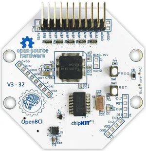
(15) CHAPTER 1. INTRODUCTION. 1.3. Materials and Methods. Our whole system is based on the Raspberry Pi1 hardware platform. Raspberry Pi is a single board computer developed by the Raspberry Pi company based in United Kingdom. Although its firmware is not open source, it allows to install a Linux based distribution. In this case we chose to install Raspbian, a distribution based on Debian, over a Raspberry Pi model 3B+. This model has an ARM Broadcomm 64-bit quad-processor @1.4GHz and 1GB of RAM. The data storage is done in a 32GB micro SD card. It supports WiFi, ethernet, bluetooth 4.2 bluetooth low energy (BLE). It could be connected to several peripherals using a HDMI or USB ports. We decided to power it via a USB connection to a powerbank (20.000 mAh) to maximize the system autonomy and mobility. This hardware offers us all the characteristics that we were looking for: it has enough computational power to carry our calculations, its small and light, it allows us to use free and open source software and is economic (32.50 e). For code development we chose Python as programming language. The major reason for this is to achieve a complete compatibility with the Python code available for the acquisition device. This is explained in the following section. Other reasons for this selection have been the large amount of libraries writen for Python and the big community behind this programming language.. 1.3.1. Acquisition. First of all we are going to explain our acquisition paradigm. We recorded 5 blocks of 15 repetitions for each action. We have 4 different actions (look up, look down, look left and look right). We ended with 75 repetitions for each action. We decided to establish a 3 second window to perform each of the actions. When the user runs the block acquisition, a beep sound is presented 5 times with a 3 seconds interval between each beep sound. This is done to show the user the frequency to perform the desired actions. After that, at the beginning of each 3 seconds window, the user will hear a voice indicating the desired action the perform. The actions are randomly distributed. The data is recorded in a file with the EOG amplitude value for horizontal and vertical components and also the label for the desired action. The hardware used for the acquisition is the OpenBCI Cyton board2 an 8-channel biosensing board. This board contains a PIC32MX250F128B microcontroller and a Texas Instruments ADS1299 analog/digital converter and amplifier. This device is distributed by OpenBCI, a USA company. A view of this device can be seen in Figure 1.5. 1 2. Raspberry Pi 3B+ official website OpenBCI Cyton official website. 9.

(16) CHAPTER 1. INTRODUCTION. Figure 1.5: OpenBCI Cyton board We decided to use this device because its gives us enough precision and sample rate (250 Hz) for our needs, is cheap compared to other EOG acquisition devices (499.99 $), it has an open-source environment (including a Python library to work with the boards3 ), it has an active and big community4 and it can be powered with a powerbank, being a light and mobile solution. For the EOG signal recording we have used 4 EMG/ECG wet electrodes connected to two channels in the board in a differential mode. Differential mode is calculating the voltage difference between the two electrodes connected to the channel and doesn’t need a reference electrode. The two channels correspond to the vertical and horizontal components of the signal. The montage used is as in Figure 1.2, using electrodes B and C as vertical channel and D and E as horizontal channel. Electrode A is not used because, as it has been said, we don’t need a reference electrode in differential mode.. 1.3.2. Signal pre-processing. When we acquire EOG signals, there is some artifacts or noises that could contaminate it, like some artificial sources, electrode’s movement, power line noise, head movement, illumination changes and so on [2][1][37]. This noises and artifacts come under high frequencies [8] and should be removed. Taking into account that EOG signal information is mainly contained in low frequencies [41] we have decided to apply a Butterworth bandpass filter with a range between 0.03 and 20 Hz and order 2. This parameters were chosen based on the results shown in Chapter 2 Table 2.1. Then, a smoothing filter is applied to reduce irregularities that carries no information. For applying the filter we have used the SciPy library, a free and open-source library including modules for linear algebra, 3 4. Github repository for OpenBCI Python code OpenBCI forum. 10.

(17) CHAPTER 1. INTRODUCTION integration, FFT or signal and image processing. SciPy is commonly used and has a big community supporting it. The last step in pre-processing was to standarize the data. This is done to remove the baseline of EOG signals [37]. The standarization was done using the following formula: Xt =. xt − µ i σi. where Xt is the resulting datapoint, xt is the datapoint value before standarization, µi is the mean value of the whole sample and σi is the standard deviation of the whole sample.. 1.3.3. Feature extraction. As it has been said, feature extraction is a key step in our system’s pipeline and it would give us the characteristics of each sample in order to maximize the inter-class separability and intra-class similarity. For this we calculate 12 features for the horizontal and vertical components of our signal, i.e. 24 total features per sample. The features are the following: • Min: The minimum value in the sample. • Max: The maximum value in the sample. • Median: The value in the sample that has as many values above as below. • Mode: The most frequent value in the sample. • Kurtosis: A statistical parameter related on the tail values of the data distribution. • Max position: The position where we found the maximum value in the sample. • Min position: The position where we found the minimum value in the sample. • Area under the curve: The value of the signal function integral. • First quartile: The value representing the 25 percentile in the data distribution. • Third quartile: The value representing the 75 percentile in the data distribution. • Interquartile range: The difference between thir and first quartile. • Derivative slope: To calculate this feature first we calculate an approximation to the derivative of the signal using the formula dxt =. xt − xt−n n. where dxt is the value of the derivative for xt datapoint, xt is the value of the datapoint, xt−n is the value n-datapoints before and n is the value of the step that. 11.

(18) CHAPTER 1. INTRODUCTION we want to use to calculate the derivative. After that, for each sample we calculate the derivative slope as ds =. kdxmax − dxmin k pos(dxmax ) − pos(dxmin ). where dxmax and dxmin are the maximum and minimum values in the sample derivative and pos(dxmax ) and pos(dxmin ) are their positions. ds will result in a negative value for EOG signals with a positive step and positive values for a EOG signal with a negative step.. 1.3.4. Classification. We decided to use a SVM classifier because of its simplicity over other methods like artificial neural networks (ANN). This simplicity decreases significantly the training time and also the classification time of a single sample, giving a lower reaction time to our system. We used a linear kernel in order to keep the classification as simple and fast as possible without compromising their accuracy. We established the penalty parameter C to 0.75 because it uses less time to build the classifier than C =1 and has the same accuracy. The selected strategy was One vs. Rest because it showed exactly the same results as One vs. One but slightly lower training time, probably due to the smaller number of classifiers that has to train. The kernel, C parameter and strategy selection was done based on the achieved accuracies that are shown in Chapter 2 Table 2.1. To obtain a better model without spending too much time on training we decided to use a 5-fold cross-validation in order to get an accuracy as high as possible and build the model using the hold dataset. For the classification step we used the SVC function included in the SVM module in Scikit-learn library. This library has a high reputation in machine learning and it has been widely used, having a lot of online examples and a huge community behind it.. 1.3.5. Control paradigm & control system. The design of our control paradigm was based on 4 different actions: look up, look down, look left and look right. We had 5 states in our state machine: Stop, move forward, move backward, move left and move right. We arrive to the movement states only from the Stop state and we arrive to the Stop state from a movement state with the look up action. The diagram of this state machine is presented in Figure 1.6 where the squares represents the actions to be performed by the wheelchair and the arrows represents the actions to be performed by the user.. 12.

(19) CHAPTER 1. INTRODUCTION. Figure 1.6: Control paradigm diagram This paradigm election implies a continuous system where an action is performed until the user selects to stop the action by looking up. We prefer this paradigm over the discrete paradigm where an action is performed for a certain amount of time or space (i.e. turn left for 2 seconds or go forward for 1 meter) because we thought it would be more comfortable and more flexible for the user . The wheelchair used in this system is the Bischoff & Bischoff Eltego5 , a light and cheap (2540 e) powered wheelchair with two independent motors, one for the left wheel and one for the right wheel. The control is made by, as usual, with a joystick. This joystick allows the user to select the movement direction and speed depending on how far the joystick is from its center. The joystick sends two signals to each motor, one to control the rotation speed and direction of the specific wheel and the other one to control the break system. The signal for the brake system takes the values 0V when the brakes are not activated and 21V when we are breaking. The signal to control the rotation speed and direction takes values between 0V and ±21V. Signal amplitude corresponds to the rotation speed. This rotation can be forward or backward depending on positive or negative amplitude values. Because of the lack of adequate equipment, in this case a certain quality oscilloscope, we were not able to do a correct characterization of the signal. We were not sure if this signal corresponds to a DC signal with an amplitude directly related to the distance between the joystick position and the joystick center or a pulse-width modulated (PWM) signal where the user modifies the duty cycle with the joystick movement. This fact, added to 5. Bischoff & Bischoff Eltego official website. 13.

(20) CHAPTER 1. INTRODUCTION the lack of time because of the delays acquiring all the materials needed to this project, resulted in the impossibility of finishing the control system.. 1.4. Task Planning. Below is detailed the task distribution on a calendar. It can be seen that weekends have been left free of work.. Figure 1.7: Task planning for February. Figure 1.8: Task planning for March. Figure 1.9: Task planning for April. 14.

(21) CHAPTER 1. INTRODUCTION. Figure 1.10: Task planning for May. Figure 1.11: Task planning for June. 1.5. Product Summary. The products developed during this work can be summarized as: 1. A complete software pipeline to acquire, pre-process and classify the EOG signals into the appropiate actions permorfed by the user. This software can be seen in the Chapter 5. 2. A software subsystem able to translate the classification into control commands for the wheelchair. As it has been explained in Section 1.3.5, this subsystem was developed due to a several time and material problems.. 1.6. Descripton of the Memory. Chapter 2 presents the results obtained for this system implementation, from pre-processing to classification. Chapter 3 will discuss this results and propose some further work to improve the system. Finally, Chapter 5 presents the most important parts of the code developed in the scope of this project.. 15.

(22)

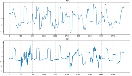
(23) Chapter 2 Results The first step after the signal acquisition was the pre-processing. Figures 2.1 and 2.2 show the same EOG signal before and after pre-processing. It can be seen that after the pre-processing it is easier to appreciate the steps in the vertical component for Up and Down eye movements and in the horizontal component for Left and Right movements. This results correspond to the results that we expected.. Figure 2.1: EOG vertical and horizontal components before pre-processing. The samples correspond to Left, Up, Left, Left, Left, Down, Right, Up, Left and Right movements. 17.

(24) CHAPTER 2. RESULTS. Figure 2.2: EOG vertical and horizontal components after pre-processing. The samples correspond to Left, Up, Left, Left, Left, Down, Right, Up, Left and Right movements After this, we permorfed the feature extraction. Figures 2.3, 2.4, 2.5 and 2.6 show the values for some of this features. We can see in Figure 2.3 and Figure 2.4 a significant difference between the values for Left and Right movements in the horizontal component and Up and Down movements in the vertical component in Minimum and Maximum features. It was expected to have a clear difference for the minimum and maximum values.. Figure 2.3: Values for horizontal (top) and vertical (bottom) components for Minimum feature. From left to right: Up, Down, Left and Right movements. 18.

(25) CHAPTER 2. RESULTS. Figure 2.4: Values for horizontal (top) and vertical (bottom) components for Maximum feature. From left to right: Up, Down, Left and Right movements It can not be seen a clear difference between the values for Left and Right movements in the horizontal component and Up and Down movements in the vertical component for Area Under the Curve (Figure 2.5) or Derivative Slope (Figure 2.6) features. This is particularly unexpected in the case of the derivative slope that should show a negative value for Left and Up signals in the horizontal and vertical components respectively and positive values for Right and Down signals in horizontal and vertical components.. Figure 2.5: Values for horizontal (top) and vertical (bottom) components for Area Under the Curve feature. From left to right: Up, Down, Left and Right movements. 19.

(26) CHAPTER 2. RESULTS. Figure 2.6: Values for horizontal (top) and vertical (bottom) components for Derivative Slope feature. From left to right: Up, Down, Left and Right movements The last process in our pipeline was to perform the classification with a 5-fold crossvalidation. We changed some of the values in the filter and the SVM classifier to find which of them were the best to build our model. The results can be seen in Table 2.1. Even that some of the features do not seem to provide any relevant information to the classifier, the system was able to achieve a 98% accuracy with an average accuracy of 93% over the 5 classifiers resulting from the cross-validation. As it is explained in Section 1.3.5, because of equipment and time issues, we were able to implement the control subsystem. Due to this fact, no results on this subsystem are presented in this section.. 20.

(27) CHAPTER 2. RESULTS. Filter 0.01-20 0.05-20 0.1-20 0.03-20 0.04-20 0.03-35 0.03-25 0.03-20 0.03-20 0.03-20 0.03-20 0.03-20 0.03-20 0.03-20 0.03-20 0.03-20 0.03-20 0.03-20 0.03-20 0.03-20 0.03-20 0.03-20 0.03-20 0.03-20 0.03-20. Order 2 2 2 2 2 2 2 3 4 2 2 2 2 2 2 2 2 2 2 2 2 2 2 2 2. Kernel Linear Linear Linear Linear Linear Linear Linear Linear Linear Linear Linear Linear Linear Linear RBF RBF Polynomial 2-degree Polynomial 2-degree Polynomial 3-degree Polynomial 5-degree Polynomial 10-degree Polynomial 25-degree Polynomial 50-degree Linear Linear. Strategy One vs. One One vs. One One vs. One One vs. One One vs. One One vs. One One vs. One One vs. One One vs. One One vs. One One vs. One One vs. One One vs. One One vs. One One vs. One One vs. One One vs. One One vs. One One vs. One One vs. One One vs. One One vs. One One vs. One One vs. Rest One vs. Rest. C 1 1 1 1 1 1 1 1 1 1.5 1.25 0.75 0.9 0.5 0.75 1.25 0.75 1 0.75 0.75 0.75 0.75 0.75 0.75 1. Min 0.52 0.79 0.54 0.90 0.85 0.85 0.88 0.79 0.63 0.85 0.88 0.92 0.90 0.85 0.44 0.44 0.40 0.42 0.40 0.44 0.46 0.5 0.46 0.92 0.90. Max 0.92 0.96 0.92 0.96 0.96 0.98 0.94 0.94 0.92 0.94 0.94 0.98 0.96 0.98 0.63 0.60 0.56 0.56 0.60 0.69 0.85 0.81 0.75 0.98 0.96. Average 0.82 0.88 0.80 0.93 0.88 0.90 0.90 0.85 0.79 0.91 0.92 0.93 0.92 0.92 0.53 0.54 0.52 0.51 0.52 0.55 0.61 0.65 0.60 0.93 0.93. Table 2.1: Minimum, maximum and average accuracies with 5-fold cross-validation. 21.

(28)

(29) Chapter 3 Conclusions The present project presents an acquisition, pre-processing and classification pipeline for EOG signals able to achieve a 98% classification accuracy and a 93% average accuracy for Up, Down, Left and Right movements. This method runs over a cheap, small and light hardware system, perfect to be installed in a powered wheelchair. The proposed system reaches better results than other proposed systems in the literature [38][37][42][43]. Even not all the objectives for this project have been achieved (as it has been explained in Section 1.3.5) all the objectives related to bioinformatics, biostatistics and machine learning have been solved properly.. 3.1. Future Work. Following modules need to be implemented to acheive the proposed objective: • Perform a correct caracterization of the control signals for the wheelchair. • Write the code to do an online classification of the EOG signals. • Find the appropiate device to deliver the voltage needed to control the wheelchair motors. • Write the code correspondent to the wheelchair control. Now we would like to present some ideas in order to improve the system: • Remove the not significant features from the system. This would make the system faster due to the fact that it would not performing unwanted calculations. • Find additional features. There are some features present in the literature that are not included in the system and could even improve the performance. • Try to optimize the filter process. It could be interesting to explore other filtering options.. 23.

(30)

(31) Chapter 4 Glossary ALS: Amyotrophic Lateral Sclerosis LIS: Locked-in Syndrome CLIS: Completely Locked-in State HCI: Human-Computer Interface EOG: Electrooculography IROG: Infrared Reflection Oculography HMI: Human-Machine Interface BCI: Brain-Computer Interface EMG: Electromyography EEG: Electroencephalography NIRS: Near-infrared Spectroscopy SVM: Support Vector Machine RBF: Radial Basis Function ANN: Artificial Neural Network SVC: Support Vector Classifier. 25.

(32)

(33) Chapter 5 Supplementary Material 5.1 1 2 3. Pre-processing function. import numpy a s np from s c i p y import s i g n a l from s c i p y . s i g n a l import b u t t e r , l f i l t e r. 4 5 6. import r e a d f u n c t i o n a s r e a d import s p l i t i n t o t r i a l s a s t r i. 7 8 9 10 11 12 13. 14. 15 16 17 18 19. def f i l t e r ( f i l e s , samples per trial ) : ””” # FUNCTION: filter ( files ) # INPUT : L i s t o f f i l e s t o f i l t e r and number o f s a m p l e s p e r t r i a l # OUTPUT: V e r t i c a l & h o r i z o n t a l components o f t h e data d i v i d e d by t r i a l s and a l i s t c o n t a i n i n g t h e l a b e l o f each t r i a l # DESCRIPTION : A p p l i e s a Butterworth f i l t e r and a smoothing f i l t e r o v e r t h e data i n each f i l e . Then c a l l s t o t r i a l s ( ) t o n o r m a l i z e and s p l i t into t r i a l s ””” lowcut = 0.03 h i g h c u t = 20 f s = 250 order = 2. 20 21 22 23 24 25 26 27 28 29 30 31. hor tmp = [ ] ver tmp = [ ] labels tmp = [ ] hor bnd = [ ] ver bnd = [ ] hor sm = [ ] ver sm = [ ] # Arrays with h o r i z o n t a l and v e r t i c a l components & l a b e l s o f each sample hor = [ ] ver = [ ] lab = [ ]. 32 33. p r i n t ( ” S t a r t f i l t e r i n g . Lowcut : ” , lowcut , ” Highcut : ” , h i g h c u t , ” Order : ” , order ). 27.

(34) CHAPTER 5. SUPPLEMENTARY MATERIAL 34 35 36 37. # Read f i l e by f i l e for file name in f i l e s : hor tmp , ver tmp , l a b e l s t m p = r e a d . r e a d f i l e ( f i l e n a m e ). 38 39 40. 41 42. # Butterworth bandpas f i l t e r f i l e by f i l e s o s = s i g n a l . b u t t e r ( o r d e r , [ lowcut , h i g h c u t ] , ’ bandpass ’ , a n a l o g=F a l s e , output= ’ s o s ’ , f s =250) hor bnd = s i g n a l . s o s f i l t ( s o s , hor tmp ) v e r b n d = s i g n a l . s o s f i l t ( s o s , ver tmp ). 43 44 45. 46 47. # Butterworth bandpas f i l t e r f i l e by f i l e # [ b , a ] = s i g n a l . b u t t e r ( o r d e r , [ lowcut , h i g h c u t ] , ’ bandpass ’ , a n a l o g= F a l s e , output =’ba ’ , f s =250) # hor bnd = s i g n a l . f i l t f i l t ( b , a , hor tmp ) # v e r b n d = s i g n a l . f i l t f i l t ( b , a , ver tmp ). 48 49 50 51 52 53 54 55. # Smoothing f i l t e r f i l e by f i l e hor sm = s i g n a l . m e d f i l t ( hor bnd , k e r n e l s i z e = 3 5 ) ver sm = s i g n a l . m e d f i l t ( ver bnd , k e r n e l s i z e = 3 5 ) # Concatenate t h e r e s u l t s i n t o v e r and hor v a r i a b l e s & l a b e l s hor . extend ( hor sm ) v e r . extend ( ver sm ) l a b . extend ( l a b e l s t m p ). 56 57 58. # S p l i t a l l data i n t o t r i a l s & s t a n d a r i z e o v e r t r i a l s t r i a l h o r , t r i a l v e r , t r i a l l a b = t r i . t o t r i a l s ( hor , ver , lab , samples per trial ). 59 60. return trial hor , t r i a l v e r , t r i a l l a b. 5.2 1 2. Feature extraction function. import numpy a s np from s c i p y import s t a t s. 3 4 5 6 7 8. 9 10. def features ( tr i al h or , t r i a l v e r ) : ””” # FUNCTION: features ( trial hor , trial ver ) # INPUT : H o r i z o n t a l & V e r t i c a l components o f each t r i a l # OUTPUT: Matrix with f e a t u r e v a l u e s o f h o r i z o n t a l & v e r t i c a l components o f each t r i a l # DESCRIPTION : E x t r a c t s t h e f e a t u r e s f o r each t r i a l ”””. 11 12 13. num feat = 24 # Number o f F e a t u r e s ( 1 2 v e r t i c a l and 12 h o r i z o n t a l ) f e a t u r e s = np . z e r o s ( ( l e n ( t r i a l h o r ) , num feat ) ). 14 15 16. f o r i t e r in range (0 , len ( t r i a l h o r ) ) :. 17 18 19. f e a t u r e s [ i t e r ] [ 0 ] = np . min ( t r i a l h o r [ i t e r ] ) # H o r i z o n t a l Min f e a t u r e s [ i t e r ] [ 1 ] = np . min ( t r i a l v e r [ i t e r ] ) # V e r t i c a l Min. 28.

(35) CHAPTER 5. SUPPLEMENTARY MATERIAL 20 21 22. f e a t u r e s [ i t e r ] [ 2 ] = np . max( t r i a l h o r [ i t e r ] ) # H o r i z o n t a l Max f e a t u r e s [ i t e r ] [ 3 ] = np . max( t r i a l v e r [ i t e r ] ) # V e r t i c a l Max. 23 24 25. f e a t u r e s [ i t e r ] [ 4 ] = np . median ( t r i a l h o r [ i t e r ] ) # H o r i z o n t a l Median f e a t u r e s [ i t e r ] [ 5 ] = np . median ( t r i a l v e r [ i t e r ] ) # V e r t i c a l Median. 26 27. 28. f e a t u r e s [ i t e r ] [ 6 ] = f l o a t ( s t a t s . mode ( t r i a l h o r [ i t e r ] ) [ 0 ] ) # H o r i z o n t a l Mode f e a t u r e s [ i t e r ] [ 7 ] = f l o a t ( s t a t s . mode ( t r i a l v e r [ i t e r ] ) [ 0 ] ) # V e r t i c a l Mode. 29 30. 31. f e a t u r e s [ i t e r ] [ 8 ] = s t a t s . k u r t o s i s ( t r i a l h o r [ i t e r ] , n a n p o l i c y= ’ omit ’ ) # Horizontal Kurtosis f e a t u r e s [ i t e r ] [ 9 ] = s t a t s . k u r t o s i s ( t r i a l v e r [ i t e r ] , n a n p o l i c y= ’ omit ’ ) # Vertical Kurtosis. 32 33. 34. f e a t u r e s [ i t e r ] [ 1 0 ] = i n t ( np . where ( t r i a l h o r [ i t e r ] == np . max( t r i a l h o r [ i t e r ] ) ) [ 0 ] [ 0 ] ) # H o r i z o n t a l Max p o s i t i o n f e a t u r e s [ i t e r ] [ 1 1 ] = i n t ( np . where ( t r i a l v e r [ i t e r ] == np . max( t r i a l v e r [ i t e r ] ) ) [ 0 ] [ 0 ] ) # V e r t i c a l Max p o s i t i o n. 35 36. 37. f e a t u r e s [ i t e r ] [ 1 2 ] = i n t ( np . where ( t r i a l h o r [ i t e r ] == np . min ( t r i a l h o r [ i t e r ] ) ) [ 0 ] [ 0 ] ) # H o r i z o n t a l Min p o s i t i o n f e a t u r e s [ i t e r ] [ 1 3 ] = i n t ( np . where ( t r i a l v e r [ i t e r ] == np . min ( t r i a l v e r [ i t e r ] ) ) [ 0 ] [ 0 ] ) # V e r t i c a l Min p o s i t i o n. 38 39. 40. f e a t u r e s [ i t e r ] [ 1 4 ] = sum ( abs ( t r i a l h o r [ i t e r ] ) ) # H o r i z o n t a l Area under the curve f e a t u r e s [ i t e r ] [ 1 5 ] = sum ( abs ( t r i a l v e r [ i t e r ] ) ) # V e r t i c a l Area under the curve. 41 42. 43. f e a t u r e s [ i t e r ] [ 1 6 ] = np . p e r c e n t i l e ( t r i a l h o r [ i t e r ] , 2 5 ) # H o r i z o n t a l First quartile f e a t u r e s [ i t e r ] [ 1 7 ] = np . p e r c e n t i l e ( t r i a l v e r [ i t e r ] , 2 5 ) # V e r t i c a l First quartile. 44 45. 46. f e a t u r e s [ i t e r ] [ 1 8 ] = np . p e r c e n t i l e ( t r i a l h o r [ i t e r ] , 7 5 ) # H o r i z o n t a l Third q u a r t i l e f e a t u r e s [ i t e r ] [ 1 9 ] = np . p e r c e n t i l e ( t r i a l v e r [ i t e r ] , 7 5 ) # V e r t i c a l Third q u a r t i l e. 47 48. 49. features [ iter ][20] = ( t r i a l h o r [ i t e r ] , 25) features [ iter ][21] = ( t r i a l v e r [ i t e r ] , 25). np . p e r c e n t i l e ( t r i a l h o r [ i t e r ] , 7 5 ) − np . p e r c e n t i l e # Horizontal I n t e r q u a r t i l e range np . p e r c e n t i l e ( t r i a l v e r [ i t e r ] , 7 5 ) − np . p e r c e n t i l e # V e r t i c a l I n t e r q u a r t i l e range. 50 51 52 53 54. # Calculate derivative & derivative slope d e r h o r = np . z e r o s ( l e n ( t r i a l h o r [ i t e r ] ) ) d e r v e r = np . z e r o s ( l e n ( t r i a l v e r [ i t e r ] ) ). 55 56 57 58. pos min der hor = [ ] pos max der hor = [ ] pos min der ver = [ ]. 29.

(36) CHAPTER 5. SUPPLEMENTARY MATERIAL pos max der ver = [ ]. 59 60. min max min max. 61 62 63 64. der der der der. hor hor ver ver. = = = =. 0 0 0 0. 65. f o r j in range (5 , len ( t r i a l h o r [ i t e r ] ) ) : d e r h o r [ j ] = ( t r i a l h o r [ i t e r ] [ j ] − t r i a l h o r [ i t e r ] [ j −5]) / 5 d e r v e r [ j ] = ( t r i a l v e r [ i t e r ] [ j ] − t r i a l v e r [ i t e r ] [ j −5]) / 5. 66 67 68 69 70 71 72 73. min max min max. der der der der. hor hor ver ver. = = = =. np . min ( d e r np . max( d e r np . min ( d e r np . max( d e r. pos pos pos pos. min max min max. der der der der. hor hor ver ver. hor ) hor ) ver ) ver ). 74 75 76 77 78. = = = =. i n t ( np . where ( d e r i n t ( np . where ( d e r i n t ( np . where ( d e r i n t ( np . where ( d e r. hor hor ver ver. == == == ==. min max min max. der der der der. hor ) hor ) ver ) ver ). [0][0]) [0][0]) [0][0]) [0][0]). 79 80. 81. features [ − pos min features [ − pos min. iter der iter der. ] [ 2 2 ] = abs ( max der hor − m i n d e r h o r ) / ( p o s m a x d e r h o r h o r )# H o r i z o n t a l D e r i v a t i v e S l o p e ] [ 2 3 ] = abs ( m a x d e r v e r − m i n d e r v e r ) / ( p o s m a x d e r v e r v e r )# V e r t i c a l D e r i v a t i v e S l o p e. 82 83 84. return features. 5.3 1 2 3. Classification function. from s k l e a r n . m o d e l s e l e c t i o n import t r a i n t e s t s p l i t from s k l e a r n . svm import SVC from s k l e a r n . m o d e l s e l e c t i o n import c r o s s v a l s c o r e. 4 5 6 7 8 9 10 11. 12 13. def c l a s s i f i c a t i o n ( feat , t r i a l l a b , c r o s s v a l i d a t i o n ) : ””” # FUNCTION: feature plot ( feat , to plot ) # INPUT : Matrix with t h e f e a t u r e s , l a b e l s f o r t h e t r i a l s and a b o x p l o t # i n d i c a t i n g i f we want t o do c r o s s −v a l i d a t i o n o r not # OUTPUT: Accuracy o f t h e model # DESCRIPTION : C r e a t e s an SVM model t o f i t t h e t e s t data i f ’ c r o s s v a l i d a t i o n ’ i s False # o r c r e a t e s m u l t i p l e SVM models i f ’ c r o s s v a l i d a t i o n ’ i s True ”””. 14 15 16 17 18 19 20 21. # Train model and p r e d i c t l a b e l s c = 1.25 kernel = ’ linear ’ gamma = ’ s c a l e ’ d e c i s i o n = ’ ovo ’ cv = 5 t e s t s i z e = 0 . 3 3 # Used o n l y i f. ’ c r o s s v a l i d a t i o n ’ == F a l s e. 30.

(37) CHAPTER 5. SUPPLEMENTARY MATERIAL 22 23 24 25 26. 27 28 29 30 31 32. i f c r o s s v a l i d a t i o n == True : # Cr o ss V a l i d a t i o n o v e r a l l data p r i n t ( ” C l a s s i f i c a t i o n s t a r t e d . C : ” , c , ”CV: ” , cv ) c l f = SVC(C=c , k e r n e l=k e r n e l , gamma=gamma , d e c i s i o n f u n c t i o n s h a p e= decision ) s c o r e s = c r o s s v a l s c o r e ( c l f , f e a t , t r i a l l a b , cv=cv ) p r i n t ( ”Mean Accuracy : %0.2 f ” % ( s c o r e s . mean ( ) ) ) print (” All accuracies : ” , scores ) else : # S p l i t F e a t u r e s and L a b e l s i n t o t r a i n & t e s t feat train , feat test , trial lab train , trial lab test = t r a i n t e s t s p l i t ( feat , t r i a l l a b , t e s t s i z e ). 33 34 35. 36 37. # C l a s s i f y o v e r Train & Test data c l f = SVC(C=c , k e r n e l=k e r n e l , gamma=gamma , d e c i s i o n f u n c t i o n s h a p e= decision ) clf . f i t ( feat train , trial lab train ) p r i n t ( ” Accuracy : ” , c l f . s c o r e ( f e a t t e s t , t r i a l l a b t e s t ) ). 31.

(38) Bibliography [1] Z. Lv, Y. Wang, C. Zhang, X. Gao, and X. Wu, “An ica–based spatial filtering approach to saccadic eog signal recognition,” Biomedical Signal Processing and Control, vol. 43, pp. 9–17, 2018. [Online]. Available: https: //www.sciencedirect.com/science/article/pii/S174680941830003X [2] R. Barea, L. Boquete, M. Mazo, and E. López, “System for assisted mobility using eye movements based on electrooculography,” IEEE transactions on neural systems and rehabilitation engineering, vol. 10, no. 4, pp. 209–218, 2002. [Online]. Available: https://ieeexplore.ieee.org/abstract/document/1178091/ [3] C.-W. Hsu, C.-C. Chang, C.-J. Lin et al., “A practical guide to support vector classification,” 2003. [Online]. Available: https://tinyurl.com/y3z63739 [4] A. Ben-Hur, C. S. Ong, S. Sonnenburg, B. Schölkopf, and G. Rätsch, “Support vector machines and kernels for computational biology,” PLoS computational biology, vol. 4, no. 10, p. e1000173, 2008. [Online]. Available: https://journals.plos.org/ploscompbiol/article?id=10.1371/journal.pcbi.1000173 [5] G. Logroscino, M. Piccininni, B. Marin, E. Nichols, F. Abd-Allah, A. Abdelalim, F. Alahdab, S. W. Asgedom, A. Awasthi, Y. Chaiah et al., “Global, regional, and national burden of motor neuron diseases 1990–2016: a systematic analysis for the global burden of disease study 2016,” The Lancet Neurology, vol. 17, no. 12, pp. 1083–1097, 2018. [Online]. Available: https://www.sciencedirect.com/science/article/pii/S1474442218304046 [6] B. Oskarsson, T. F. Gendron, and N. P. Staff, “Amyotrophic lateral sclerosis: an update for 2018,” in Mayo Clinic Proceedings. Elsevier, 2018. [Online]. Available: https://www.sciencedirect.com/science/article/abs/pii/S0025619618302660 [7] U. Chaudhary, B. Xia, S. Silvoni, L. G. Cohen, and N. Birbaumer, “Brain–computer interface–based communication in the completely locked–in state,” PLoS biology, vol. 15, no. 1, p. e1002593, 2017. [Online]. Available: https://journals.plos.org/ plosbiology/article?id=10.1371/journal.pbio.1002593&xtor=AL-32280680 [8] S. Bharadwaj and B. Kumari, “Electrooculography: Analysis on device control by signal processing,” International Journal of Advanced Research in Computer Science, vol. 8, no. 3, 2017. [Online]. Available: https://tinyurl.com/yyxjhxoc [9] W. Heide, E. Koenig, P. Trillenberg, D. Kömpf, and D. Zee, “Electrooculography: technical standards and applications,” Electroencephalogr Clin Neurophysiol Suppl, 32.

(39) BIBLIOGRAPHY vol. 52, pp. 223–240, 1999. [Online]. Available: https://pdfs.semanticscholar.org/ b255/0bdcb2a945769a1b5399ce5765b5035b2298.pdf [10] R. Barea, L. Boquete, S. Ortega, E. López, and J. Rodrı́guez-Ascariz, “Eog–based eye movements codification for human computer interaction,” Expert Systems with Applications, vol. 39, no. 3, pp. 2677–2683, 2012. [Online]. Available: https://www.sciencedirect.com/science/article/pii/S0957417411012541 [11] S.-L. Wu, L.-D. Liao, S.-W. Lu, W.-L. Jiang, S.-A. Chen, and C.T. Lin, “Controlling a human–computer interface system with a novel classification method that uses electrooculography signals,” IEEE transactions on Biomedical Engineering, vol. 60, no. 8, pp. 2133–2141, 2013. [Online]. Available: https://ieeexplore.ieee.org/abstract/document/6468076/ [12] Q. Huang, S. He, Q. Wang, Z. Gu, N. Peng, K. Li, Y. Zhang, M. Shao, and Y. Li, “An eog–based human–machine interface for wheelchair control,” IEEE Transactions on Biomedical Engineering, vol. 65, no. 9, pp. 2023–2032, 2018. [Online]. Available: https://ieeexplore.ieee.org/document/7994682/ [13] R. Barea, L. Boquete, M. Mazo, and E. López, “Wheelchair guidance strategies using eog,” Journal of intelligent and robotic systems, vol. 34, no. 3, pp. 279–299, 2002. [Online]. Available: https://link.springer.com/article/10.1023/A:1016359503796 [14] C. W. Hess, R. Muri, and O. Meienberg, “Recording of horizontal saccadic eye movements: methodological comparison between electro– oculography and infrared reflection oculography,” Neuro-ophthalmology, vol. 6, no. 3, pp. 189–197, 1986. [Online]. Available: https://www.tandfonline. com/doi/abs/10.3109/01658108608997351?casa token=sfu UJJFWiIAAAAA: y0fCUU0mQoWas5mEptJYPvF6QBopFFQrJnSmcQ4iWAofHDAkigOz sURdTYKSgSuDQq4GhD1ofvY [15] K. Arai and R. Mardiyanto, “A prototype of electric wheelchair controlled by eye–only for paralyzed user,” Journal of Robotics and Mechatronics, vol. 23, no. 1, p. 66, 2011. [Online]. Available: https://www.researchgate.net/ profile/Kohei Aarai/publication/267790510 A Prototype of Electric Wheelchair Controlled by Eye-Only for Paralyzed User/links/54d9e9360cf25013d04360b5/ A-Prototype-of-Electric-Wheelchair-Controlled-by-Eye-Only-for-Paralyzed-User. pdf [16] C. Kolski and E. Le Strugeon, “A review of intelligent human–machine interfaces in the light of the arch model,” International Journal of Human-Computer Interaction, vol. 10, no. 3, pp. 193–231, 1998. [Online]. Available: https: //www.tandfonline.com/doi/pdf/10.1207/s15327590ijhc1003 1?needAccess=true [17] Z. Hossain, M. M. H. Shuvo, and P. Sarker, “Hardware and software implementation of real time electrooculogram (eog) acquisition system to control computer cursor with eyeball movement,” in 2017 4th International Conference on Advances in Electrical Engineering (ICAEE). IEEE, 2017, pp. 132–137. [Online]. Available: https://ieeexplore.ieee.org/abstract/document/8255341/ 33.

(40) BIBLIOGRAPHY [18] H. S. Dhillon, R. Singla, N. S. Rekhi, and R. Jha, “Eog and emg based virtual keyboard: A brain–computer interface,” in 2009 2nd IEEE International Conference on Computer Science and Information Technology. IEEE, 2009, pp. 259–262. [Online]. Available: https://ieeexplore.ieee.org/abstract/document/5282570 [19] L. M. Argentim, M. C. F. Castro, and P. A. Tomaz, “Human interface for a neuroprothesis remotely control.” in BIODEVICES, 2018, pp. 247–253. [Online]. Available: https://www.scitepress.org/papers/2018/67190/67190.pdf [20] U. Chaudhary, N. Birbaumer, and A. Ramos-Murguialday, “Brain–computer interfaces for communication and rehabilitation,” Nature Reviews Neurology, vol. 12, no. 9, p. 513, 2016. [Online]. Available: https://www.nature.com/nrneurol/journal/ v12/n9/abs/nrneurol.2016.113.html [21] A. Larson, J. Herrera, K. George, and A. Matthews, “Electrooculography based electronic communication device for individuals with als,” in 2017 IEEE Sensors Applications Symposium (SAS). IEEE, 2017, pp. 1–5. [Online]. Available: https://ieeexplore.ieee.org/abstract/document/7894062/ [22] M. Rokonuzzaman, S. Ferdous, R. A. Tuhin, S. I. Arman, T. Manzar, and M. N. Hasan, “Design of an autonomous mobile wheel chair for disabled using electrooculogram (eog) signals,” in Mechatronics. Springer, 2011, pp. 41–53. [Online]. Available: https://link.springer.com/chapter/10.1007/978-3-642-23244-2 6 [23] R. Barea, L. Boquete, L. M. Bergasa, E. López, and M. Mazo, “Electro– oculographic guidance of a wheelchair using eye movements codification,” The International Journal of Robotics Research, vol. 22, no. 7–8, pp. 641–652, 2003. [Online]. Available: https://journals.sagepub.com/doi/abs/10.1177/ 02783649030227012?casa token=s5CmPdr9f5kAAAAA:tQAwOfgWVJO9W80W E41V8pcY63vPcvoWux7hVImhr8TTbKu0 cY64SuE8bq8V6jqw2TpUPmKVb[24] S. Yathunanthan, L. Chandrasena, A. Umakanthan, V. Vasuki, and S. Munasinghe, “Controlling a wheelchair by use of eog signal,” in 2008 4th International Conference on Information and Automation for Sustainability. IEEE, 2008, pp. 283–288. [Online]. Available: https://ieeexplore.ieee.org/abstract/document/4783987/ [25] M. Mazo, F. Rodrı́guez, J. Lázaro, J. Ureña, J. C. Garcia, E. Santiso, and P. Revenga, “Electronic control of a wheelchair guided by voice commands,” Control Engineering Practice, vol. 3, no. 5, pp. 665–674, 1995. [Online]. Available: https://www.sciencedirect.com/science/article/abs/pii/096706619500042S [26] Y. Matsumotot, T. Ino, and T. Ogsawara, “Development of intelligent wheelchair system with face and gaze based interface,” in Proceedings 10th IEEE International Workshop on Robot and Human Interactive Communication. ROMAN 2001 (Cat. No. 01TH8591). IEEE, 2001, pp. 262–267. [Online]. Available: https://ieeexplore.ieee.org/abstract/document/981912/ [27] J. Rosen, M. Brand, M. B. Fuchs, and M. Arcan, “A myosignal–based powered exoskeleton system,” IEEE Transactions on systems, Man, and Cybernetics–part 34.

(41) BIBLIOGRAPHY A: Systems and humans, vol. 31, no. 3, pp. 210–222, 2001. [Online]. Available: https://ieeexplore.ieee.org/abstract/document/925661 [28] A. Ferreira, W. C. Celeste, F. A. Cheein, T. F. Bastos-Filho, M. Sarcinelli-Filho, and R. Carelli, “Human–machine interfaces based on emg and eeg applied to robotic systems,” Journal of NeuroEngineering and Rehabilitation, vol. 5, no. 1, p. 10, 2008. [Online]. Available: https://jneuroengrehab.biomedcentral.com/articles/10. 1186/1743-0003-5-10 [29] G. Gallegos-Ayala, A. Furdea, K. Takano, C. A. Ruf, H. Flor, and N. Birbaumer, “Brain communication in a completely locked–in patient using bedside near–infrared spectroscopy,” Neurology, vol. 82, no. 21, pp. 1930–1932, 2014. [Online]. Available: https://n.neurology.org/content/82/21/1930.short [30] H. Erkaymaz, M. Ozer, and İ. M. Orak, “Detection of directional eye movements based on the electrooculogram signals through an artificial neural network,” Chaos, Solitons & Fractals, vol. 77, pp. 225–229, 2015. [Online]. Available: https://www.sciencedirect.com/science/article/pii/S0960077915001691 [31] B. E. Boser, I. M. Guyon, and V. N. Vapnik, “A training algorithm for optimal margin classifiers,” in Proceedings of the fifth annual workshop on Computational learning theory. ACM, 1992, pp. 144–152. [Online]. Available: https://dl.acm.org/citation.cfm?id=130401 [32] V. Vapnik, S. E. Golowich, and A. J. Smola, “Support vector method for function approximation, regression estimation and signal processing,” in Advances in neural information processing systems, 1997, pp. 281–287. [Online]. Available: https://tinyurl.com/yxwcqx6t [33] S.-i. Amari and S. Wu, “Improving support vector machine classifiers by modifying kernel functions,” Neural Networks, vol. 12, no. 6, pp. 783–789, 1999. [Online]. Available: https://www.sciencedirect.com/science/article/pii/S0893608099000325 [34] A. Ben-Hur and J. Weston, “A users guide to support vector machines,” in Data mining techniques for the life sciences. Springer, 2010, pp. 223–239. [Online]. Available: https://link.springer.com/protocol/10.1007/978-1-60327-241-4 13 [35] C.-W. Hsu and C.-J. Lin, “A comparison of methods for multiclass support vector machines,” IEEE transactions on Neural Networks, vol. 13, no. 2, pp. 415–425, 2002. [Online]. Available: http://web.cs.iastate.edu/∼honavar/multiclass-svm.pdf [36] R. Kohavi et al., “A study of cross–validation and bootstrap for accuracy estimation and model selection,” in Ijcai, vol. 14, no. 2. Montreal, Canada, 1995, pp. 1137–1145. [Online]. Available: https://www.researchgate.net/profile/ Ron Kohavi/publication/2352264 A Study of Cross-Validation and Bootstrap for Accuracy Estimation and Model Selection/links/02e7e51bcc14c5e91c000000.pdf [37] L. J. Qi and N. Alias, “Comparison of ann and svm for classification of eye movements in eog signals,” in Journal of Physics: Conference Series, 35.

(42) BIBLIOGRAPHY vol. 971, no. 1. IOP Publishing, 2018, p. 012012. [Online]. Available: https://iopscience.iop.org/article/10.1088/1742-6596/971/1/012012/meta [38] X. Guo, W. Pei, Y. Wang, Y. Chen, H. Zhang, X. Wu, X. Yang, H. Chen, Y. Liu, and R. Liu, “A human–machine interface based on single channel eog and patchable sensor,” Biomedical Signal Processing and Control, vol. 30, pp. 98–105, 2016. [Online]. Available: https://www.sciencedirect.com/science/article/pii/S1746809416300787 [39] S. Aungsakul, A. Phinyomark, P. Phukpattaranont, and C. Limsakul, “Evaluating feature extraction methods of electrooculography (eog) signal for human–computer interface,” Procedia Engineering, vol. 32, pp. 246–252, 2012. [Online]. Available: https://www.sciencedirect.com/science/article/pii/S1877705812012957 [40] P. Phukpattaranont, S. Aungsakul, A. Phinyomark, and C. Limsakul, “Efficient feature for classification of eye movements using electrooculography signals,” Therm. Sci, vol. 20, pp. 563–572, 2016. [Online]. Available: http://thermalscience.vinca.rs/ pdfs/papers-2016/TSCI151005038P.pdf [41] M. Merino, O. Rivera, I. Gómez, A. Molina, and E. Dorronzoro, “A method of eog signal processing to detect the direction of eye movements,” in 2010 First International Conference on Sensor Device Technologies and Applications. IEEE, 2010, pp. 100–105. [Online]. Available: https://ieeexplore.ieee.org/abstract/ document/5632116/ [42] R. Barea, L. Boquete, J. M. Rodriguez-Ascariz, S. Ortega, and E. López, “Sensory system for implementing a human–computer interface based on electrooculography,” Sensors, vol. 11, no. 1, pp. 310–328, 2011. [Online]. Available: https://www.mdpi.com/1424-8220/11/1/310 [43] A. R. Kherlopian, J. P. Gerrein, M. Yue, K. E. Kim, J. W. Kim, M. Sukumaran, and P. Sajda, “Electrooculogram based system for computer control using a multiple feature classification model,” in 2006 International Conference of the IEEE Engineering in Medicine and Biology Society. IEEE, 2006, pp. 1295–1298. [Online]. Available: https://ieeexplore.ieee.org/abstract/document/4461997/. 36.

(43)