An open source browser based software tool for graph drawing and visualisation

Texto completo

(1)An open source browser-based software tool for graph drawing and visualisation Master Thesis submittet to the Department of IT, Multimedia and Telecommunications of the Universitat Oberta de Catalunya in partial fulfillment of the requirements for the academic degree of Master in Free Software by Veit-Dieter VOGT Supervisor / Tutor Prof. C. Garrigues Olivella 2014.

(2) Declaration Hereby I certify that I have conducted this Master Thesis independently and used no other than the specified resources.. Veit-Dieter Vogt.

(3) Table of Contents Abstract.................................................................................................................1 1 Introduction........................................................................................................3 2 Graph Drawing and Visualisation......................................................................5 3 Methodology....................................................................................................21 3.1 In-detail description of the data analysis..............................................23 3.1.1 Identifying the candidates.........................................................24 3.1.2 Reading existing reviews..........................................................24 3.1.3 Comparing the leading programs.............................................25 3.1.4 In-depth analysis of the top candidates....................................26 4 I R C A..............................................................................................................27 4.1 Identify..................................................................................................27 4.2 Read Reviews......................................................................................28 4.3 Comparison..........................................................................................30 4.3.1 Functionality..............................................................................30 4.3.2 Market share.............................................................................30 4.3.3 Support / Maintenance / Longevity / Reliability........................31 4.3.4 Flexibility / Customisability........................................................33 4.3.5 Licence.....................................................................................35 4.3.6 Other cirteria.............................................................................36 4.4 Analysis in-depth..................................................................................37 4.5 Conclusion............................................................................................39 5 Software Development....................................................................................41. i.

(4) 5.1 Unified Modeling Language (UML)......................................................43 5.1.1 Use Cases Diagram.................................................................45 5.1.2 Sequence Diagram...................................................................48 6 Documention of the software tool....................................................................51 6.1 Installation in 4 steps............................................................................51 6.2 Workspace, Toolbar and Properties.....................................................58 6.3 The Menu Bar.......................................................................................60 6.4 Graph edit options................................................................................68 6.5 To Do List..............................................................................................76 6.6 General Features.................................................................................76 7 References.......................................................................................................81 Appendix A..........................................................................................................89 The BSD 3-clauses licence........................................................................89 Appendix B..........................................................................................................95 The MIT licence..........................................................................................95 Appendix C..........................................................................................................97 The Mozilla Public Licence Version 2........................................................97 Appendix D........................................................................................................111 The GNU General Public Licence Version 2............................................111 Appendix E........................................................................................................127 The GNU General Public Licence Version 3............................................127 Appendix F........................................................................................................157 Public Domain..........................................................................................157. ii.

(5) Table of Figures Picture 1: Portrait of Leonard Euler by Emmanuel Handmann 1753...................5 Picture 2: City Map of Königsberg........................................................................6 Picture 3: Marked Bridges....................................................................................6 Picture 4: First Step of Abstraction.......................................................................6 Picture 5: Second Step of Abstraction..................................................................6 Picture 6: Non-planar Graph.................................................................................9 Picture 7: Planar Graph........................................................................................9 Picture 8: Graph with many crossings................................................................10 Picture 9: Graph with less crossings...................................................................10 Picture 10: Planarised Graph..............................................................................10 Picture 11: Symmetric Graph..............................................................................11 Picture 12: Proximity Drawing.............................................................................12 Picture 13: Graph drawn as Tree........................................................................13 Picture 14: The same graph drawn in an other manner.....................................13 Picture 15: Straight-line graph drawing..............................................................13 Picture 16: L-, T- and Z-shape rectagular graph drawings.................................15 Picture 17: Force-directed graph drawing..........................................................16 Picture 18: 3D graph drawing.............................................................................18 Picture 19: Labeled Graph..................................................................................19 Picture 20: Example of an Use Cases Diagram.................................................46 Picture 21: Use Cases Diagram of the software tool..........................................47 Picture 22: Example of a Sequence Diagram.....................................................49. iii.

(6) Picture 23: Sequence Diagram of the software tool...........................................50 Picture 24: Greedy installation initial picture.......................................................52 Picture 25: Not all requirements are fulfilled.......................................................53 Picture 26: All requirements fulfilled....................................................................54 Picture 27: Nothing to do....................................................................................54 Picture 28: Data for administration not completed.............................................55 Picture 29: Data input completed........................................................................55 Picture 30: Admin account created successfully................................................56 Picture 31: Installation is finished.......................................................................56 Picture 32: Greedy login window........................................................................57 Picture 33: User data inserted............................................................................57 Picture 34: The initial screen of greedy..............................................................58 Picture 35: Toolbar and Properties turned off.....................................................59 Picture 36: Toolbar with item "Edges" choosen..................................................60 Picture 37: Menu bar with item Files selected....................................................62 Picture 38: Menu bar with item Edit choosen.....................................................63 Picture 39: View item of the menu bar................................................................64 Picture 40: Menu item Algorithms selected........................................................65 Picture 41: Item Options in the menu bar selected............................................66 Picture 42: List of template graphs.....................................................................66 Picture 43: Graph K5 selected from list..............................................................67 Picture 44: Item Help in menu bar selected with information about the licence.68 Picture 45: New node created............................................................................69 Picture 46: A new graph was created.................................................................70 Picture 47: Dijkstra algorithm selected in the Algorithms item...........................71. iv.

(7) Picture 48: A new Dijkstra grid was generated...................................................72 Picture 49: The start node is marked (green node in upper left corner).............73 Picture 50: After the end node (red node in lower right corner) was marked the calculation starts (gray and yellow nodes)..........................................................74 Picture 51: Calculation of the shortest path is finished (red nodes)...................75. v.

(8) List of Tables Table 1: Identification of the Libraries.................................................................28 Table 2: Data which indicate the market share of the libraries...........................31 Table 3: Support information about the libraries.................................................33 Table 4: Licences of the libraries........................................................................35 Table 5: Licence compatibility.............................................................................36 Table 6: Feature list of libraries...........................................................................38 Table 7: Used libraries and their licences...........................................................77. vi.

(9) vii.

(10)

(11) Abstract. Abstract One objective of this master thesis was to find and evaluate open source tools or libraries for graph visualisation which are qualified for educational purposes. This tool should be capable for a prospective graph theory course. The open source libraries have to support graph drawing and visualisation and can run in a browser. First there was a comprehensive search where a lot of libraries were found. Not all of them are under an open source licence, these were filtered off. Secondly these libraries which are written in a computer language which can not run in a browser were separated. These, written in Javascript, which remain subsequently were evaluated to find out which one is the best for this task. The result was that d3.js is that library which has the greatest functional range, best flexibility and could be easily customised. The second intension was to develop an open source software tool where d3.js was included as graph drawing and visualisation library. The software was written in Javascript so that it can run browser-based. With this tool the students ought to do their exercises and homework. In order not to begin from scratch and develop the entire software, tools and work which are already had been developed and which can be found in the internet was used and integrated. But there was one essential condition to acquit: These tools or software snippets must be under an open source licence and all the licences must be compatible! Finaly the graph drawing and visualisation editor was presented.. 1.

(12) 2.

(13) 1 Introduction. 1. Introduction. Graph visualisation is an interesting field of mathematics. With graph visualisation one can show the relationships among the elements of interest. These relationships can be unidirectional or bidiredional, which means that these relations can have one way from one element to an other only, or the elements have interrelations. It is not only of academic interest, but also referes to many aspects of our real-life briefly. With graph visualisation scientists can show the manifold links among users of social networks, clarify the connections of PCs, servers and other network devices among a computer network, or even the internet, illustrate the biological structures of a united cell structure, point up the neural structure of a brain or biological formation. Software dependencies of a complex software meshwork could be elucidated. Graph visualisation can also show the organisational hierarchies in human and animalistic societies, as there are enterprises, residents of a city or an entire nation and of a flock or a swarm. There are many other fields of application in industry and science. Since Big Data is a buzzword in IT, data visualisation is more necessary than before. Today it is no problem to aquire such an amount of data that humans can not interprete these data without visualisation. Graph visualisation plays a major role in this context. One intension of this master thesis was to find and evaluate open source tools or libraries for graph visualisation which are qualified for educational purposes, i.e. for teaching a graph theory course. After a comprehensive search these libraries which do not fit the requirements are filtered off. Adjacent the remaining 3.

(14) 1 Introduction libraries were evaluated which one is the best for a graph drawing and visualidation tool. The second goal was to develop a software tool for the intended graph theory course which can run in a browser. The students ought to download this tool from the UOC's virtual campus. With this software tool they will than do their exercises and homework. In order not to begin from scratch and develop the entire software, tools and work which have already been developed and which can be found in the internet was used and integrated. But there was one essential condition to acquit: These tools or software snippets must be under an open source licence and all the licences must be compatible!. 4.

(15) 2 Graph Drawing and Visualisation. 2. Graph Drawing and Visualisation. A Review of the current research Around 1736 some citizen of Königsberg (today Kaliningrad) asked whether it was possible to make a city tour by using every bridge exactly one time only. Königsberg at that time had 7 bridges. The mathematician Leonard Euler (1707 – 1783) attented to this question. Euler gave some thoughts to this problem and established hereby the mathematical section of graph theory. He took a city map of Königsberg, marked the bridges and then he drew an abstracted map of the city and at the end he drew points and lines to finish the abstraction. Picture 1: Portrait of Leonard Euler He figured out, that for a solution every point by Emmanuel Handmann 1753 must have an equal number of incoming and outgoing ways. Which means that the number of connections of a point must be even. But some of the points have odd connections so that his definite answer was that it is not possible to take this city tour.. 5.

(16) 2 Graph Drawing and Visualisation. Picture 2: City Map of Königsberg. Picture 3: Marked Bridges. Picture 4: First Step of Abstraction. Picture 5: Second Step of Abstraction. The pictures 2 to 5 illustrates Euler's way of abstraction of the Königsberg bridges problem. ( All pictures taken from en.wikipedia.org ) Today these points and lines are called nodes and edges. Graph theory developed in the last centuries to a veritable research field in mathematics. With the increasing number of nodes and edges in a graph it was more and more unreal to understand a graph without visualising them, because humans do understand things better if they can see them. By graph visualisation it is pos-. 6.

(17) 2 Graph Drawing and Visualisation sible to show the different relationships among the elements of interest. These relationships can be unidirectional or bidirectional, which means that the relations can be one-way or see-saw. Graph visualisation today is not only of academic interest. With graph visualisation you can show the manifold links among people using social networks, or it could clarify the connections of computers, servers and other devices in a computer network, or the internet in total. Graph visualisation illustrates the biological structures of a united cell structure, points up the neural structure of a brain, or a biological formation. Graph visualisation elucidates software dependencies of a complex software meshwork, or the line drawings of electronic circuits. Graph visualisation can also show the organisational hierarchies in human and animalistic societies, enterprises, residents of a city or an entire nation and of a flock or a swarm. The research field of graph drawing and visualisation is separated into several section problems: •. planarity testing and embedding. •. crossings and planarisation. •. symmetric graph drawing. •. proximity drawing. •. tree drawing algorithms. •. planar straight-line drawing algorithms. •. planar orthogonal and polyline drawing algorithms. •. spine and radial drawing 7.

(18) 2 Graph Drawing and Visualisation •. circular drawing algorithms. •. rectangular drawing algorithms. •. simultaneous embedding of planar graphs. •. force-directed drawing algorithms. •. hierarchical drawing algorithms. •. three-dimensional drawing algorithms and. •. labeling algorithms.. The following review will report the current research of graph drawing and visualisation and will reveal open questions in the sections. Planarity testing and embedding The characterisation of a planar graph was written in the 1930s [Kur30], but it took a long time since 1970 [HT74] to find a linear-time solution. Why are planar graphs so interesting? They have several interesting properties. Planar graphs are sparce and 4-colorable [AH77]. Their inner structure can be described very easy and the less crossings a graph has the better is its readability for humans. Therefore the testing of planarity of a graph is an interesting research field. There are some algorithms for testing the planarity. All linear-time algorithms fall into two categories. One category is called cycle based and the other one vertex addition algorithm. The cylce based technique is that a cycle splits the graph into two sections, an inner and an outer section. The technique of the vertex addition algorithms is to beginn with smaller planar graphs and than adding vertices to build the final graph [HT08]. Depth First Search (DFS) is a technique which is common to all planarity testing methodes. It is a special method to vistit 8.

(19) 2 Graph Drawing and Visualisation all vertices of a graph in specified order. Recognising a planar graph is a main problem. Is a graph certified as non-planar it is called a Kuratowski subgraph isolation [CMS08]. Scientists have developed dynamic algorithms to determine the planarity of a graph (Lempel-Even-Cederbaum [LEC67], Shih-Hsu [SH99] and Boyer-Myrvold [BM04]). Computing planar embeddings means that vertices and edges are added or deleted to construct the final graph [DBTV01].. Picture 6: Non-planar Graph. Picture 7: Planar Graph. In planarity testing there are some constraints in simultaneous planarity testing, clustered planarity testing and decomposition-based planarity testing. Crossings and planarisation Another problem is that the bigger the graph and the more crossings it has the lesser is the readability. Crossing minimisation is an optimisation problem in graph drawing. This problem was first examined by Turan during World War II. There are some algorithms which try to solve the problem, but it is still an open problem. Crossing minimisation is as well of commercial interest. In VLSI (very large scale integration) design it is necessary to have as less crossings as possible. More wire crossings imply more costs of the chip. The planarisation method [BTT84] is the current approach to the crossing minimisation problem. 9.

(20) 2 Graph Drawing and Visualisation This method consists of two steps. The first step is to draw a planar subgraph which has as many edges as possible. All edges which are not contained in this drawing will then be inserted in the next step. Whenever a crossing is produced, a dummy vertex will be inserted to eliminate the crossing. After all edges have been inserted a planar drawing algorithm will than compute the layout. At the end the dummy vertices will be deleted.. Picture 8: Graph with many crossings. Picture 9: Graph with less crossings. One of the open problems in crossing minimisation is the determination of the crossing numbers of the final graph [PT00]. Another problem is the approximability of crossing minimisation.. Picture 10: Planarised Graph. Symmetric graph drawing Drawing a graph symmetrically is in most cases preferred by humans over a planar graph drawing [KK89]. Therefore symmetry graph drawing is another. 10.

(21) 2 Graph Drawing and Visualisation important section in graph drawing and is based on fundamental aesthetic criteria. The goal is it to find besides the trivial symmetry a non-trivial symmetry of a graph [CLY01]. Symmetries are related to the automorphisms of a graph. A symmetry can be rotational or reflective or a combination of both. An automorphism group of a graph defines these combinatorial symmetries. But not every automorphism can be drawn as a symmetric graph. A goal of symmetric graph drawing is to determine the automorphisms of a graph which can be drawn symmetricaly. Drawing a graph „very very symmetric“ is one of the open problems. If there are two drawings of a graph with the same symmetry that one is preferred which has the more elaborated symmetry but the scientists are far away from designing an algorithm to draw a graph „very Picture 11: Symmetric Graph. very symmetric“.. Proximity drawing Proximity graph drawing is another question in graph visualisation. A geometric graph which is drawn straight-line and build by a group of nodes where pairs of nodes are connected is called a proximity graph when they have a defined proximity. Depending on the definition of closeness, the same set of nodes could lead to a variety of proximity graphs. Motivated by numerous scientific applications [GO04] [Tou05] [CPZ04] scientists try to efficiently compute different types of proximity graphs of a given set of nodes. The goal is to design an efficient algorithm for computing a proximity graph drawing which is called the proximity. 11.

(22) 2 Graph Drawing and Visualisation drawability problem. Research area of proximity graph drawing is far from solving the problems. There are many questions which are unanswered. For example: minimum weight drawings [MS92], Delaunay and Voronoi drawings [SIII00], ß-drawings [Rad88], sphere of influence drawings Picture 12: Proximity Drawing. [HJLM93], rectangle of influence drawings. [LLMW98] and other proximity rules. Today this section of proximity graph drawing follows two research directions: One is the question of proximity drawings and ad-hoc networks, and the other question is that of proximity drawings and geometric checkers. Tree drawing algorithms For the purposes of representation of relational informations a tree drawing of a graph is suited. In such a tree a node represents an entity and an edge that of the association between the entities. These hierarchical informations could be a program nesting tree, an organisation chart, an activity tree, a knowledge-representation isa hierarchy, a structure of a website, an evolutionary tree, a molecular drawing, or indexes of databases. Typically an algorithm for tree. 12.

(23) 2 Graph Drawing and Visualisation drawing is based on the understanding of the structure of the tree. Also aestethic aspects are important for tree drawing because the readability and Picture 13: Graph drawn as Tree. under-standebility depends on an aesthetical. drawing. Several types of approaches are used to descibe the different hierarchical informations. They are the level-based approach [BJL02], the path-based approach [GR03a], the ring circular layout approach [GADM04] and the separation-based approach [RS07]. There are special algorithms to draw binary trees too. A. Picture 14: The same graph binary tree is a tree where every node has one drawn in an other manner or two children only [Mac03]. Planar straight-line drawing algorithms Already in the 1930s investigations had been undertaken to do planar straight-line drawings [SR34]. The results had shown, that every planar graph allows a planar straight-line drawing. Today there are two major algorithms to draw graphs straight-line: The shift method [dFPP90] and the realizer method [Sch90], an improved method of realizer was introduced later [BFM07].. Picture 15: Straight-line graph drawing. 13.

(24) 2 Graph Drawing and Visualisation Planar orthogonal and polyline drawing algorithms Drawing a planar orthogonal graph has the advantage that the graph has no crossings and the angles between the edges are 90° or 180°. But on the other side it also has the disadvantage that the graph can have a degree of a maximum of 4 only. Drawing a graph planar orthogonal is of industrial interest because VLSI design uses planar orthogonal graph drawing for the routing of the wires on a chip. More general are the polyline drawings of a graph. In this kind of drawing the edges can have angles of 45° and the multiple. These graphs than can have degrees of more than 4. There are different algorithms to draw an planar orthogonal graph: The network flow technique [GT02] and the mixed-model algorithm [GM98]. Spine and radial drawing Directed graphs which edges are parallel straight lines are called spine drawings of graphs. Drawings of directed graphs where the edges are concentric circles are called radial drawings. These two kinds of graph drawings belong to the family of layered graph drawing. One of the problems is the point-set embeddability which is investigated in computational geometry [Bos02]. Also not solved are some theoretical connetions between spine and radial drawings. Problems in graph theory and compu-tational geometry are unanswered too [DDLW05] [Sug02]. Circular drawing algorithms If the following three conditions are fulfilled, a graph drawing is called a circular graph drawing: a. the graph is partitioned into clusters, b. the nodes of each. 14.

(25) 2 Graph Drawing and Visualisation cluster are placed onto the circumference of an embedding circle and c. each edge is drawn as a straight line. For the calculation of circular graph drawings there are two efficient algorithms [Bra97] [DMM97]. The scientists could show that these algorithms work very well in applied practices and produce drawings with a low number of edge crossings [ST06]. Rectangular drawing algorithms A graph where the vertices are drawn as points and the edges are drawn as horizontal or vertical lines only and the graph is a planar graph, than this graph drawing is called a rectangular graph drawing. This drawing has practical applications in VLSI floorplannings like chip design or architecture [NR04].. Picture 16: L-, T- and Z-shape rectagular graph drawings On a chip with sections which produces heat these sections should not be adjacent so that the heat dissipation can work sufficently [She95]. Another practical application is the floorplanning of buildings. For example should the cafeteria not be adjacent to laboratories where it is deald with poisonous chemicals [FW74]. There are several drawing algorithms in practice which deliver good results [KH97] [LL90]. Simultaneous embedding of planar graphs In cases where not only one graph could explain the relations between the ver15.

(26) 2 Graph Drawing and Visualisation tices there are two or more graphs which share some or even all vertices needed to describe the situation. This is called a simultaneous embedding of planar graphs. The question than is how could these graphs be best displayed. Because there are various scenarios which need different layouts not only one algorithm could satisfy all particular layouts. For a proper layout the scientists have to take into account the readability and the mental map preservation. These two criteria are often contradictory. The readability is an aspect of aestethic, e. g. the minimal number of crossings. The mental map preservation could be achieved by keeping the vertices of consecutive graphs at the same position. Optimising the one is to downgrade the other. It is essential to keep a balance. Simultaneous embeddings of graphs have much applications in sciences: software engineering, databases, or social networks. Also in industry the simultaneous graph embeddings are of interest. VLSI design uses such algorithms to solve the optimisation problem of chip placement [MOS98]. In this section there are many open problems. Force-directed drawing algorithms If there are forces between the vertices of a graph it is to bespoken of force-directed graphs. These forces could be repulsive or attractive between vertices which are adjacent. Force-directed algorithms have a long history in this research field. Already in the 1960s algorithms to calculate Picture 17: Forcedirected graph In the last years there had been good progress and many drawing force-directed graph drawings were introduced [Tut63].. 16.

(27) 2 Graph Drawing and Visualisation improved algorithms had been implemented [Ead84] [FR91]. But these algorithms work good for graphs with only a few vertices but not if the graphs have hundreds or even thousands of vertices. One of the obstacle is that the physical models have more than one minimum and even with sophisticated mechanisms it is not possible to get good layouts for bigger graphs. Since the late 1990s there had been introduced better algorithms which now can handle graphs with thousands of vertices. These layouts consist of a series of simple graphs so that the readability of the whole composition is acceptable [Wal03] [GGK04]. Also some algorithms do not use Euclidean geometry, but the surface of a sphere or a torus [KW05]. The newer scalable algorithms which can handle large dynamic graphs with thousands of vertices are used in many applications [Mun97]. Hierarchical drawing algorithms A special case of a directed graph is a hierarchical graph drawing. Examples for hierarchical graphs are the organisation of an enterprise, function calls of a software, object-oriented class diagrams or a PERT chart of a project management. The major algorithm for drawing hierarchical graphs is the Sugiyama method [STT81]. In the last years there had been many modifications and enhancements of this framework [dNE02] [SM95a] [UBSE98]. But all these alternatives have their special applications and limitations. There are attempts to draw hierarchical graphs in 3D [GT97] [HN05a]. One of several approaches to overcome these limitations is the UPL system [CGMW11]. So-called radial level drawings are another alternative method for visualisation of a social network [BKW03]. The cycle style of drawing was also introduced to avoid the top-. 17.

(28) 2 Graph Drawing and Visualisation to-bottom leveling [BBBL08]. Three-dimensional drawing algorithms In most cases it is sufficient to draw a graph in two dimensions. But for special applications a drawing in three dimensions is better. These applications could be VLSI design [LR86], software engineering [WHF93] or information visualisation [WM08]. 3D drawings have made great advantages in the last years by better hard-. Picture 18: 3D graph drawing. ware and increasing computer power. So-called grid-drawings, that are graph drawings where the vertices have integer co-ordinates only, ensure a minimum of grid spacing and the readability is better if the nodes would be too adjacent. Another aspect of 3D drawing is straight-line crossing-free graph drawing. Orthogonal drawings have edges which are parallel to one of the axis and they guarantee a good angular resolution. In VLSI design it is important to minimise the space for the chip to avoid dissipation of space. There are still many open problems in 3D graph drawing but with increasing computer power the scientists had made good progress in the last decades. Labeling algorithms Automated labeling edges and nodes is a major problem in graph drawing. Labeling has for example applications in cartography [RMM+95] and geographic information systems (GIS) [Fre91].. 18.

(29) 2 Graph Drawing and Visualisation In cartography the labeling is elevated into an art over the decades and automatic labeling never will reach a sufficent placement. But in some cases like real-time placement in on-line GIS, oil exploration [Zor90] or internet-based mapping it has acceptable qualitiy. At present time the semi-automated labeling systems are the best approach. They produce an initial labeling and adjacent it will be improved manually. By increasing computer capabilities the automated labeling will make. Picture 19: Labeled Graph. further advances.. Conclusion In graph drawing and visualisation the scientists have made good progress in the last decades. The theoretical basics in information technology has been augmented in the last sixty years. Some new languages in artificial intelligence have been developed to better support the implementation of algorithms for graph drawings. The efficiency of the algorithms has been improved over the time and the computational capabilities progressed with seven-league boots. But still there are several questions without an answer. The research field of graph drawing and visualisation is still an interesting field of research and will show some appealing and instructive changes over the next years. Note: All pictures in this chapter are taken from [Tam13]. 19.

(30) 20.

(31) 3 Methodology. 3. Methodology. In this Master Thesis we searched for documents about the libraries, evaluate them and decided which of them is the best for developing our tool. This first part is a document approach. The second part of the research work is a design and creation approach. Here we develop a tool for the intended graph theory course of the UOC. Stol and Babar [SB10] listed 20 Open Source Software evaluation methods. Some of them are industry driven and do not cover the intentions for the special purpose here. Others are very comprehensive and sophisticated; these are not suited to be taken into account in this research work because it would take too long to get familiar with these methods. Among the remaining there are the papers of Cruz, Wieland and Ziegler [CWZ06], the paper QSOS initiated by Atos Origin [Atos13] and the online paper of David Wheeler [Whe11] which describe methods for evaluations of free software / open source software. A first glance at these three papers showed that many points of the different methods are similar to the method described by D. Wheeler. All three methods look very much alike and only differ in some special points. The QSOS method ( see www.qsos.org ) is under an open source licence and provides a plug-in for Firefox. This tool could ease and facilitate the evaluation process. [ADDENDUM: End of May the European Commission anounced the open source project OSSmeter ( https://joinup.ec.europa.eu/elibrary/case/ossmeterplatform-automatically-assess-monitor-and-compare-oss-packages ). From the description: “Evaluating whether an open source software package meets the requirements for a specific application, or determining the best match from a list 21.

(32) 3 Methodology of packages, requires information on both the quality and the maturity of the software, as well as understanding whether the software is continuing to evolve and if there is a substantial and active community of users and developers......” For this research work it is too late to take this project into account and include more information, but furhter research should not disregard it.] Our decision therefore was to evaluate the software according D. Wheeler's IRCA method. For a detailed description see below. Regrettably we have not found any papers where researchers report that they had used Wheeler's method and we only found two papers where researchers describe their evaluation process of open source software. These are the papers of Graf and List: An Evaluation of Open Source E-Learning Platforms Stressing Adaptation Issues [GL05] and of Fleischfresser: Evaluation von Open Source Projekten: Ein GQM-basierter Ansatz [Flei07]. Due to this low number of references it is not possible to speak of a state-of-the-art in this research field. David A. Wheeler elaboratedly described in his paper “How to Evaluate Open Source Software / Free Software Programs.” a general 4-step process for evaluating programs. He calls this method “IRCA”. IRCA is a short form of: Identify the candidtes, Read existing Reviews, Compare the leading programs and Analyse the top candidates in more depth. This method will be used to evaluate the open source candidates for graph visualisation. In this paper Wheeler described 14 criteria of evaluation. Not all of them may be relevant for UOC to use the open source software / libraries in a graph theory course. In this paper he gives specific informations on how to evaluate open source software / free software (OSS/FS). Wheeler developed this process so that anyone can compare OSS/FS side-by-side with proprietary software and determine which of the can-. 22.

(33) 3 Methodology didates best meets one's needs. After an introduction about open source software, other approaches for evaluation and a short overview over the IRCA process, he goes into depth in the following four chapters. In chapter two he declares the process step of identifying the candidates and gives some tips. In chapter three he recommends to read reviews about the candidates. Briefly compare the leading program's attributes to your needs is the title of chapter four. This chapter is very detailed. In 14 subchapters he describes important attributes to be considered including functionality, cost, market share, support, maintenance, reliability, performance, scaleability, useability, security, flexibility / customisability, interoperability, and legal / licence issues. The last step in his method is to perform an in-depth analysis of the top candidates which the author discusses in chapter 5. Chaptert 6 terminates Wheeler's paper. Therein he recommends some hints how to present the results of the evaluation.. 3.1. In-detail description of the data analysis. David Wheeler called his method the IRCA method. IRCA is short for the four steps of which the method consists: 1. Identify the candidates 2. Read existing Reviews 3. Compare the programs' basic attributes and 4. Analyse the top candidates in depth. But before the researcher begins with step one, it has to be clear what requirements the candidates must comply with. Wheeler strongly recommends that the researcher who evaluates free software / open source software according his. 23.

(34) 3 Methodology method must have a basic idea of what his needs are, i.e. the researcher should have a list where all the requirements of the candidates are listed and according to which the search and evaluation will be geared to.. 3.1.1 Identifying the candidates In this first step the researcher has to do a comprehensive search, preferably in the internet, to find as many candidates as possible which roughly fulfill the requirements. Wheeler had listed some recommendations which can be an assistance for this search, e.g. a paper of the U.S. government and lists of socalled GRAM and GRAS (GRAM = generally recognised as mature) (GRAS = generally recognised as safe) software. At the end the researcher has to deselect the software which is not adequate, so that only these candidates remain, which absolutely accomplish with the researcher's needs.. 3.1.2 Reading existing reviews Wheeler's references are to visit the programs website, to read software comparisons to find the strengths and weaknesses of the candidates and he gives some examples. In our case where we search for software tools and libraries which can run in a browser and which have to be under an open source licence there are no such reviews to find. The only comments about the candidates which we had found are these in the forums. But these comments do not have any scientific explanatory power.. 24.

(35) 3 Methodology. 3.1.3 Comparing the leading programs After the candidates that do not fulfill the requirements have been eliminated the next step is a comparison. For this comparison, step three of the IRCA method, Wheeler recommends to visit the projects web page. Most open source software projects have such a web page where most of the informations about the project can be found. There you will find the documentation of the software, FAQs, mailing lists on which the researcher could subscribe to receive an impression on “what is going on” in the software project and much more. Wheeler lists here 13 facts to take into account for this comparison: functionality, cost, market share, support, maintenance, reliability, performance, scalability, usability, security, exibility/customisability, interoperability and legal / licence issues. Not all of them are relevant for my research work. Costs, market share, support, maintenance and scalability are of less or even no importance for this special comparison. The attribute legal / licence issues were a prerequirement to fulfill, a candidate which does not fit this KO criterion does not remain on the list at this stadium. The other attributes: functionality, reliability, performance, usability, security, exibility / customisability, interoperability will now be examined in more depth. Therefore all necessary informations about the candidates will be accumulated wherever it can be found resulting in a matrix which shows the most important functionalities and features. The result of this matrix is that some of the candidates will be cancelled, e.g. because of less features, or other weaknesses.. 25.

(36) 3 Methodology. 3.1.4 In-depth analysis of the top candidates This fourth and last step of Wheeler's IRCA method is the most important step because eventually a decision has to be made on which of the candidates fulfill the requirements best for the intended graph theory course. For this step Wheeler recommends to have a second but more in-depth comparison as in the previous step. He also recommends a try-out of the software. For our research work the functionality and the customisability are very important attributes. To get these informations is fundamental. In this step we had a look for special features which are important for the graph theory course: Labels, graph manipulation and graph drawing algorithms. At the end of this ultimate decision we chose the d3.js library, because this library is the most evolved one among the candidates, it has the greatest functionality and its customisability is best.. 26.

(37) 4IRCA. 4. IRCA. In this research work we had to find and compare libraries which can run with a web-based framework in a browser. These libraries have to be under an open source licence. For this comparison we will operate like D. Wheeler suggested in his paper: „How to evaluate Open Source Software / Free Software (OSS/FS) Programs.“ [Whe11].. 4.1. Identify. Our first search quarried numerous libraries from which we firstly sorted out those which are under proprietary licences. Ten libraries which are under open source licences are left then. The first six are written in Javascript and they can run in a browser. Igraph is written in C, neo4j in Java and OGDF and PIGALE in C++, they can not run in a browser, so that we did not investigate them any further. The remaining libraries we subjected to a comprehensive comparison. In Table 1 there are listed the libraries and some informations about them.. 27.

(38) 4IRCA Library. URL. Language Licence. Latest version. D3.js. d3js.org. Javascript BSD3clauses. 3.4.1. graphdracula graphdracula.net. Javascript MIT. 0.0.3alpha5. jointjs. jointjs.com. Javascript MPLv2. 0.8.0. jsdot. code.google.com/p/jsd Javascript MIT ot. 0.9. jsplumb. jsplumbtoolkit.com. Javascript MIT/GPLv2. 1.5.5. Sigma.js. sigmajs.org. Javascript MIT. 1.0.0. igraph. igraph.sourceforge.net C. GPLv2. 0.6.5. neo4j. neo4j.org. Java. GPL, but community edition only. 2.0.0. OGDF. ogdf.net. C++. GPL. 2012.7. PIGALE. pigale.sourceforge.net C++. GPL. 1.3.15. Table 1: Identification of the Libraries. 4.2. Read Reviews. D3.js Searching the internet for „d3.js review“ lead to more than 4.400.000 hits. This first impression shows the high profile of d3. There are comments to find like: „D3.js is way more than just another visualization framework.“ Many other comments which praise d3 could be found. Graphdracular To find reviews about graphdracula is in contrast a difficult task because most. 28.

(39) 4IRCA hits concern „Graf Dracula“ and not the graph visualisation library. Beside the graphdracula webpage there are almost a dozen pages where the library is the theme. Jointjs For jointjs google delivers afterall 92.900 hits. It is a relatively unknown library. Jsdot Jsdot, which was a small project at google summer of code in 2009, has just 805 hits. It will not longer be developed further so that we leave it out of deeper investigations. Jsplumb Jsplumb has 163.000 hits. The project started in November 2011 and has less than 10 contributors. So we can say that it is a small project and the development seems to be slow. Sigma.js Sigma.js is much more known. Google delivers approximately 16.200.000 hits. Sigma.js is a new and lightweight library to draw graphs. The most reviews are warm to sigma.js which had just reached version 1.0.0. The only comments about the candidates which we found are these in the forums. But these comments do not have any scientific explanatory power. The only conclusion which can be drawn is an qualitative one: Are the voices major-. 29.

(40) 4IRCA itarian pro, which means the commentator does praise the software due to its manifold features, or the commentator is contra, which means he/she criticises the program due to some bad bugs, lack of features etc. But on the basis of the number of comments it is possible to figure out the popularity of the software: The more positive comments, the greater the popularity. And from the popularity of a software it is legal to conclude to its market share.. 4.3. Comparison. 4.3.1 Functionality On https://github.com/mbostock/d3/wiki/API-Reference you can find a very long list of API-References. This list with allmost 620 entries in 39 sections shows all the functions which are included in d3. We did not find an API-Reference for graphdracula. The API-Reference for jointjs is just 77 entries long. This is not that much. At the scantily project webpage of jsdot there is no information about an API-Reference to find. The API list of jsplumb counts almost 300 entries. At sigmas webpage there is no information about an API-Reference. The functionality of the candidates is very diverse. While jsdot has only basic functions, jsplumb is more developed. Independant of the negative information about the APIs sigma is in the midfield, graphdracula has sophisticated graph drawing functions, but the best functionality by far has d3.js.. 4.3.2 Market share It is hard to evaluate the market share of open source software because there is no vendor which publishes sales volumes. But the numbers of releases and 30.

(41) 4IRCA contributors could give a first impression about the popularity and the mightiness of a forum and its activity are indices for the market share of an open source program. In the following list we have summarised some information which we found to indicate the market share.. Source developers / contributors. d3.js. graph dracula. jointjs. jsdot. jsplumb. sigma.js. github. github. github. project webpage. github. github. 67. 6. 10. 5. 7. 2. 2011 Feb17. n. a.. 2011 Feb27. n.a.. 2010 Mar15. n.a.. 164. 1. 7. 2. 22. 1. 2014 Jan14. 2011 Jun30. 2014 Jan20. 2009 Dec18. 2013 Dec06. 2014 Jan30. 22065. 332. 641. 392. 1333. 1793. releases first numbers latest github downloads. Table 2: Data which indicate the market share of the libraries D3.js is the project with the most developers / contributors, releases and downloads. This entitles to the assumption that d3.js is that library with the greatest market share.. 4.3.3 Support / Maintenance / Longevity / Reliability An index for the support, maintenance, longevity and reliability can be the ver31.

(42) 4IRCA sion number of the program and the activeness of its community. Also whether there are demos / examples and tutorials. D3.js has reached version 3.4.1 which is an indication for an long development and the maintainer M. Bostock and the large community of contributors show that the development of d3 will go on. There is a great community where questions of users are answered and the further development is discussed. On the webpage there are numerous demos and examles and a lot of tutorials. Graphdracula is still in the first steps of its development, it has just reached 0.0.3alpha5 and this release is two years old. There is no indication when it will come up to version 1.0 and it is unclear how many contributors carry the development on. There are two demos only and the documentation is in the source code only. Jointjs also has a low version number: 0.8.0. But there is an active community so that there is a justifiable hope that its development will go on. On their webpage there are 10 demos but the documentation is less. Jsdot was a litte code project in 2009 and has reached version 0.9 but it will not be developed any further. No demos are to be found on the homepage and the documentation is rather small. Jsplumb has overcome version number 1 and is now at 1.5.5. The webpage gives the impression of professionality and there is an active community in its forum. Some demos and a substancial documentation is on the webpage. Sigma.js has just reached version 1.0.0. It is a relatively new library but its popularity is increasing. Sigma is one of several projects of the medialab at Sciences Po in Paris. This leads the hope towards an ongoing development. On sigmas webpage there are only 2 demos and the documentation is not so. 32.

(43) 4IRCA much. In the table below these results are sumed up:. d3.js. graph dracula. jointjs. jsdot. jsplumb. sigma.js. demos / examples. very much. 2. 10. no. some. 2. tutorials / documentation. very much. in code only. yes. less. detailed. less. Table 3: Support information about the libraries All attempts to get in contact with the project maintainers via eMail asking for commercial support failed. There had been no replies. We gather from that that the projects do not offer commercial support for the libraries. The only support available is that from the forums and from the community. The quality of support can be infered from the activity of the community. But to set up a rank order is rarely possible, because it depends on many unpredictable factors.. 4.3.4 Flexibility / Customisability D3.js On https://github.com/mbostock/d3/wiki/Tutorials there are a lot of tutorials for d3.js on general and special themes, blogs, talks and videos, meetups and publications. If there is a function the user needs, which is not implemented, it is easy to write a plug-in for d3.js. The flexibility and customisability of d3.js is very 33.

(44) 4IRCA extensive. Graphdracula On http://www.graphdracula.net/documentation/ you may read about the documentation: „Don’t hesitate to dive into the source code! It is well described with comments and the library archive also includes some example files worth checking out.“ This means in other words: There is no documentation as that which is included in the source code. For graphdracula there are no plugins as it is to read here: „Dracula is a set of tools to display and layout interactive graphs, along with various related algorithms. No Flash, no Java, no plug-ins. Just plain JavaScript and SVG.“ [ see http://www.graphdracula.net ] Flexibility and customisability of graphdracula is therefore non-existent. Jointjs The documentation and available tutorials keep within a low limit: http://jointjs.com/tutorial. There are just 8 plug-ins listed on the webpage. Flexibility and customisability of jointjs is small. Jsdot On the scantily project's webpage there are neither informations about an APIReference, documentation nor plugins to find. Due to the fact that the project will not be developed further the flexibility and customisability of jsdot is nonexistent.. 34.

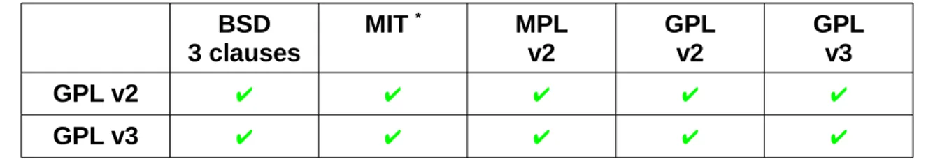
(45) 4IRCA Jsplumb The documentation on http://jsplumbtoolkit.com/doc/home is very comprehensive. But there is no information about plug-ins. Flexibility and customisability of jsplumb is better than of jointjs but much less than of d3.js. Sigma.js On sigmas webpage there are neither informations about an API-Reference nor plugins to find. But github lists 6 plugins. The tutorial is lean. Documentation is one page only: https://github.com/jacomyal/sigma.js/wiki. The flexibility and customisability of sigma is at the time out of recognition.. 4.3.5 Licence All libraries are under an open source licence as was the strict requirement. The following table shows the licences.. licence. d3.js. graph dracula. jointjs. jsdot. jsplumb. sigma.js. BSD 3 clauses. MIT. MPLv2. MIT. MIT / GPLv2. MIT. Table 4: Licences of the libraries All licences are compatible with GNU GPLv2 and v3. See table below:. 35.

(46) 4IRCA BSD 3 clauses. MIT *. MPL v2. GPL v2. GPL v3. GPL v2. ✔. ✔. ✔. ✔. ✔. GPL v3. ✔. ✔. ✔. ✔. ✔. Table 5: Licence compatibility The reader may read more information about all licences and the licence texts in Appendices A to F at the end of this document.. 4.3.6 Other cirteria D. Wheeler listed some more criteria in his paper. There are costs, performance, scaleability, useability, security and interoperability. The most of them are not relevant for this research. For instance costs: All libraries are under an open source licence and therefore no licence fee is to pay. Of course there are costs of installation and maintenance of the software but these costs are the same for other (proprietary) software. Other criteria are the performance, the useability and the security of the libraries which are dependent mainly on the program which includes the libraries. In the end there is the interoperability. The program which calls the library will run in a browser. Because it is an open source program only these browsers which are under an open source licence as well will be supported.. *The MIT licence is also known as X licence or as X11 licence. 36.

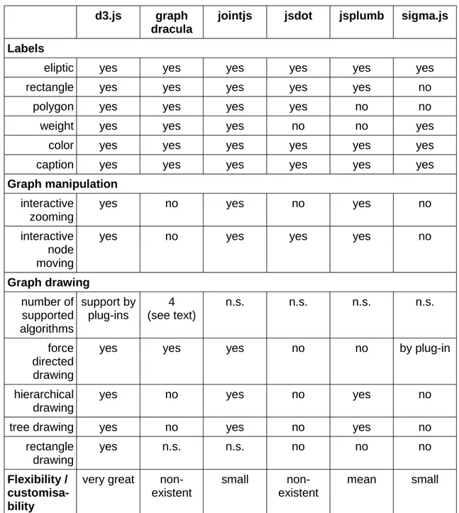
(47) 4IRCA. 4.4. Analysis in-depth. All the above listed information about the candidates is of general interest. We will now analyse the candidates for special features which are necessary for graph drawing and visualisation. First of all there is the question of labels for nodes and edges: Which labeling does the library support? Eliptic, rectangle, polygon drawing of a node and weight for an edge, color and caption for both? Graph manipulation functionality is the next question: Do the candidates support interactive zooming and interactive node moving? A very important question is the question for the integrated graph algorithms or whether it is possible to integrate graph drawing algorithms by plugins or any other mechanism. The table below indicates these features. Only graphdracula has implemented 4 graph drawing algorithms in its code. These algorithms are: Path finding (Dijkstra), shortest path (Bellman-Ford), max-flow-min-cut (Ford-Fulkerson) and string matching (Knuth-Morrison-Pratt). This list shows the functionality of the candidates. It is clear to see that d3.js has the most functions integrated and graph drawing algorithms can easily be inserted by plug-ins. Here is the web-link for a first step to write plug-ins for d3.js: http://bost.ocks.org/mike/chart. Graphdracula and jsdot have no flexibility and / or customisability. Jsplumb has a mean flexibility and customisability and that of jointjs and sigma is small.. 37.

(48) 4IRCA d3.js. graph dracula. jointjs. jsdot. jsplumb. sigma.js. eliptic. yes. yes. yes. yes. yes. yes. rectangle. yes. yes. yes. yes. yes. no. polygon. yes. yes. yes. yes. no. no. weight. yes. yes. yes. no. no. yes. color. yes. yes. yes. yes. yes. yes. caption. yes. yes. yes. yes. yes. yes. Labels. Graph manipulation interactive zooming. yes. no. yes. no. yes. no. interactive node moving. yes. no. yes. yes. yes. no. n.s.. n.s.. n.s.. n.s.. Graph drawing number of support by 4 supported plug-ins (see text) algorithms force directed drawing. yes. yes. yes. no. no. by plug-in. hierarchical drawing. yes. no. yes. no. yes. no. tree drawing. yes. no. yes. no. yes. no. rectangle drawing. yes. n.s.. n.s.. no. no. no. very great. nonexistent. small. nonexistent. mean. small. Flexibility / customisability. Table 6: Feature list of libraries. 38.

(49) 4IRCA. 4.5. Conclusion. Jsdot's development is discontinued. Graphdracula is still at the beginning and it is not clear whether it will develop. There is one developer only and it seems that he has discontinued the development. Jointjs is a small project with just 10 developers and its flexibility is small. Sigma.js is a new graph drawing project which may have a good future but its current flexibility is small. Probably it will improve. Jsplumb has also got only 7 developers but it seems the development will improve its features. Far away from the other candidates is d3.js. Its functionality and flexibility is much better than all the other libraries which we investigated. It is easy to write plug-ins for d3.js so any needed function can be integrated. D3.js is our favorite to implement as library into the web-based framework.. 39.

(50) 40.

(51) 5 Software Development. 5. Software Development. To develope software it is necessary to choose a methodical approach. There are different requirements for this approach: •. structure the development of a model to partial tasks and steps. •. use special means of representation. •. give a guidance for the realisation of the modeling. •. support the quality assurance of the models or includes critetia for „good“ models. •. as a general rule no algorithm (in mathematical meaning). •. support the relevant partial models and their integration. •. efficiency. In the development of a model the following numerous steps including repetitions and returns are generally used: •. definition of the object to model. •. determination of the modeling purpose. •. determination of the modeling environment / instruments of characterisation. •. appointment of the rules for the abstraction. •. determination of the reproduction of the reality to the modeling environment. •. testing of the model. 41.

(52) 5 Software Development There are different views for modeling of information systems: Function view ( also known as process view ): Describes the functions and partial functions prescinded from time and sequence. Sequence view ( also known as dynamic view ): Describes what activities and processes coincidentaly or consecutively execute prescinded from the semantic of the data. Data view: Describes the data which is treated or stored during a process or information system prescinded from time and independent of the sequence view. Object view: Describes a process or an information system as an amount of interacting objects prescinded from sequence, integration of data and function view. Organisation view: Describes the sequence of an organisational unit which is part of a process or information system. The communication and managerial authority correlations between the units are part of the organisational structure. Performance view: Describes the results of the process execution by product models. The purpose of such a model is: 1. To understand the reality (actual condition) •. to describe the benefit of the assumption. •. to explore the forecast about the behaviour. •. to evaluate / analyse the assignment of faults. 2. To construct the reality (target state) 42.

(53) 5 Software Development •. describing the requirements for the construction. •. analysing / simulating the examination of the construction before realisation. •. analysing potential / alternative representations of the reality. •. co-ordinating the involved persons ( customer, construtor, co-ordination between different employees / organisations, which execute the realisation co-operative ). One of these modeling languages for specification, visualisation, construction and documentation of (information) systems is the Unified Modeling Language (UML). 5.1. Unified Modeling Language (UML). UML is a standard of the OMG ( http://www.omg.org/uml ) . It is not a method , but a notation and semantics for specification, visualisation, construction and documentation of models for business processes, object orientated software development and other general systems. Like in all other languages there is a language range that kind what terms are part of the language and what denotation these terms have. This is the same what we know from other languages. But there is an important difference: While in other programing languages key words are real words, UML is a language that consists of simple geometric symbols. In UML there are defined numerous geometric forms like rectangle, arrows and ellipses and there are definitions of 43.

(54) 5 Software Development the denotation of these forms. UML knows rules how to combine these forms so that they will result in something meaningful. With these models the software developers can inspect a cut of an entire system, which important aspects will be highlighted and which unimportant aspects will be disregarded. This model is not a rebuild of the original, but a simplified description of the original with the goal to better understand the original. 13 types of diagrams are defined in UML. These diagram types are either structure diagrams or behaviour diagrams. The following six diagram types are structure diagrams: •. classes diagram. •. object diagram. •. component diagram. •. composition structure diagram. •. distribution diagram. •. packages diagram. Behaviour diagrams are the following seven diagrams:. 44. •. use case diagram. •. activity diagram. •. finite automation. •. sequence diagram. •. communication diagram. •. timing diagram.

(55) 5 Software Development •. interaction diagram. The modeling of software should aid to keep an overview. This diagram types should describe the software from different views. All together they show an overall picture of the software. Models are complied with requirements and are based of elements of the UML. The language range is independent of programing languages and platforms. The built models of software are hence independent of this technologies too. UML is also suited as co-ordinating instrument. Every developer will understand the UML models. Since UML is a graphical modeling language it is suited to communicate to non-technical persons (management) too. In the following we will restrict to show the use cases diagram and the sequence diagram of the software tool we are developing. Because JavaScript does not know the classes concept a classes diagram is not possible.. 5.1.1 Use Cases Diagram A use cases diagram consists of a lot of use cases and describes the relations between actors and use cases. A use cases diagram shows the externally visible behaviour of the system from the view of the users. Use cases will be represented by ellipses which hold the name of the use case and an amount of joint objects (actors). Any use case will be characterised in text form, more or less detailed. The correspondent use cases and actors will 45.

(56) 5 Software Development be connected by lines. The system limits are symbolised by a frame. Some use cases include further use cases, or will be extented by others. Example of an use cases diagram:. Picture 20: Example of an Use Cases Diagram In the software tool which we developed the students are the actors (and the system administrator). The user and graph databases are used for user login and logout and for up- and downloading graphs. Additionally there may be a system administration tool via which the system administrator administrates the system, e.g. the user and the graph databases (this is not part of our software). The use cases of this software are:. 46. •. user login (includes the user database). •. editing a graph. •. upload a graph (includes the graph database).

(57) 5 Software Development •. download a graph (includes the graph database). •. system administration. •. user logout (includes the user database). Editing a graph imbeds the following tasks: Changing the features of nodes and edges like shape, line, text, style, colour and weight. Nodes can be arranged in force-directed or fixed graph layout. Documenting a graph includes editing of text discribing a graph and embedding of images. The use cases diagram is shown here.. Picture 21: Use Cases Diagram of the software tool. 47.

(58) 5 Software Development. 5.1.2 Sequence Diagram A sequence diagram describes the chronology of interactions between a lot of objects within a temporal limited context. The objects will be visualised by rectangles from which the vertical life lines originate, depicted by dashed lines. The messages will be described by horizontal arrows between the life lines of the objects. At this arrows the messages will be noted in the form: message(arguments). Messages which are answers have the form: answer:=message(). Messages can also be allocated conditions by the form: [condition] message(). Iterations of messages will be depicted by a „*“ before the name of the message. Objects which are just active in interactions will be marked by a bar in the life line. An example is shown on the next page. In this software there are the students as actors, the user database which stores the allowed users and their passwords, the graph database where is stored an amount of example graphs and the students graphs. The intercations are: •. user login. •. graph editing as loop of numerous minor tasks. •. uploading a graph. •. downloading a graph. •. user logout. The sequence diagram is shown on the nextbut one page.. 48.

(59) 5 Software Development. Picture 22: Example of a Sequence Diagram. 49.

(60) 5 Software Development. Picture 23: Sequence Diagram of the software tool. 50.

(61) 6 Documention of the software tool. 6. Documention of the software tool. The purpose of the graph tool is: •. Drawing and editing graphs. •. Representation of graph theoretical structures. •. Visual representation of graph algorithms. 6.1. Installation in 4 steps. Prerequirements before installation: •. LAMP (XAMP) has to be installed. Instead of MySQL the user can also install SQLite or PostgreSQL.. •. Apache2 must be running.. •. Extraction of greedy.tar.gz to /var/www/. •. Directory /var/www/greedy, all subdirectories and files has to be owned by www-data or current apache user respectively. (command: chown -R www-data:www-data /var/www/greedy). •. The rights of /var/www/greedy/core/db have to be 777. If the users security policies do not allow 777, 755 would be good too. (command: chmod -R 777 /var/www/greedy/core/db). After the user has extracted the files to /var/www/ he has to insert “localhost/greedy” in a browser. The installation process will then start with an initial picture.. 51.

(62) 6 Documention of the software tool. Picture 24: Greedy installation initial picture He than just has to click on the arrow to proceed. In step 1 all requirements will be scanned. As long as not all requirements are fulfilled the user will see red lights as is presented in the next picture.. 52.

(63) 6 Documention of the software tool. Picture 25: Not all requirements are fulfilled When there are green lights only as seen in the following picture the user may click to continue. Otherwise the displayed problems nust be resolved. This steps have to be repeated as often as necessary by clicking on the arrow in top right corner.. 53.

(64) 6 Documention of the software tool. Picture 26: All requirements fulfilled In step 2 in the current state, the user has nothing to do just click the arrow.. Picture 27: Nothing to do In further releases, the installation can support MySQL and/or PostgreSQL as 54.

(65) 6 Documention of the software tool database systems too. The data for administration has to be inserted in step 3.. Picture 28: Data for administration not completed As long as not all required data is inserted the user will get an error message and cannot proceed to the next step.. Picture 29: Data input completed After a click on “Submit” the user will see the next picture.. 55.

(66) 6 Documention of the software tool. Picture 30: Admin account created successfully A click on OK will terminate the installation and the user can proceed after confirmation to the last step with the login to greedy.. Picture 31: Installation is finished Here the user has to insert his username and password.. 56.

(67) 6 Documention of the software tool. Picture 32: Greedy login window. Picture 33: User data inserted With the last click on “Login” the user will see the initial screen of greedy.. 57.

(68) 6 Documention of the software tool. Picture 34: The initial screen of greedy (The displayed graph is for testing purposes only, in the final version the workspace will be blank.) Now the user may begin to work with greedy.. 6.2. Workspace, Toolbar and Properties. In the centre there is the workspace. Right and left of it you find the toolbar and the area where the properties can be displayed and edited for the selected node. Both can be turned off and on.See picture 35. (The property “Location” cannot be edited, it is for information only.) In the toolbar, which is an accordion mechanism, there are the items “General” for selection of a graph element and to insert text or an image. Under the item. 58.

(69) 6 Documention of the software tool. Picture 35: Toolbar and Properties turned off “Nodes” the user can select a node, or choose one of the four node shapes: circle, square, diamond or triangle, to create an new node. Under the item “Edges” it is possible to select an edge, or to create a new edge as straight line or jagged line. See picture 36. On the right side of the workspace there is the properties area, where the name of the graph can be altered and the node properties lable, tooltip, font, colour, shape and size can be changed. Below the properties area there is a slider with which the graph can be zoomed in and out (currently this feature is not enabled, it is on the To-do-list, but instead the user can zoom in and out with the mouse wheel).. 59.

(70) 6 Documention of the software tool. 6.3. The Menu Bar. In the menu bar above the workspace there are the items: File, Edit, View, Algorithms, Options and Help. The item “File” contains: “New” to create a new graph, “Open” and “Save” to. Picture 36: Toolbar with item "Edges" choosen down- and up-load a graph from the graph database which can be located at UOC, “Save as...” to save a graph with a different name, “Import” and “Export” to load and save a graph on the local computer and “Logout” to quit greedy. See picture 37. Next is the item “Edit” where nodes, edges or “all” can be selected for demonstration purposes. See picture 38. The third item in the menu bar is “View”. Here the toolbar and properties can be 60.

(71) 6 Documention of the software tool selected to be displayed or not. See picture 39. “Algorithms” is the next item in the menu bar. Here the user can choose an algorithm to apply to a graph. Currently only the Dijksta algorithm (shortest path) is implemented (description see below). More algorithms can be integrated easily. See picture 40. The last but one item in the menu bar is the “Options” item. Here it is possible to change a graph's drawing from fixed to force-directed. If the hook at “Fix selected node” is set and a force-directed graph is drawn and the user had moved a node to another position than this node will be fixed at this position. The third item in Options is “Generate graphs”. Here the user can choose template graphs from a list. See pictures 41 and 42. As an example the graph K5 is selected in picture 43. The most right item in the menu bar is “Help”. Here the user will find the help sytem (not yet fully integrated) and the information about the licence and a link to it. See picture 44.. 61.

(72) 6 Documention of the software tool. Picture 37: Menu bar with item Files selected. 62.

(73) 6 Documention of the software tool. Picture 38: Menu bar with item Edit choosen. 63.

(74) 6 Documention of the software tool. Picture 39: View item of the menu bar. 64.

(75) 6 Documention of the software tool. Picture 40: Menu item Algorithms selected. 65.

(76) 6 Documention of the software tool. Picture 41: Item Options in the menu bar selected. Picture 42: List of template graphs 66.

(77) 6 Documention of the software tool. Picture 43: Graph K5 selected from list. 67.

(78) 6 Documention of the software tool. Picture 44: Item Help in menu bar selected with information about the licence. 6.4. Graph edit options. The following features are implemented in the graph editor: The user can draw graphs interactively and load graphs. a. from server site database (central) b. import / export (JSON format, jpeg format). To create a new graph the user has to choose “Nodes” from the toolbar, select one of the shapes and subsequently to click anywhere on the workspace. To create more nodes these steps have to be repeated until all nodes are created. See picture 45.. 68.