Stock markets, banks and economic growth in a context of common shocks and cross country dependencies

Texto completo

(1)www.iaes.es. Stock Markets, Banks and Economic Growth in a Context of Common Shocks and Cross-Country Dependencies Diego-Ivan Ruge-Leiva and Giuseppe Caivano. SERIE DOCUMENTOS DE TRABAJO 03/2017.

(2) Stock Markets, Banks and Economic Growth in a Context of Common Shocks and Cross-Country Dependencies. STOCK MARKETS, BANKS AND ECONOMIC GROWTH IN A CONTEXT OF COMMON SHOCKS AND CROSS-COUNTRY DEPENDENCIES1. ABSTRACT Although a great deal of research has shown how stock markets and banks may relate to economic growth, such studies ignore the role that common shocks play in the finance-growth nexus. Using panels of 54 advanced and emerging economies, and novel common factor frameworks which account for dynamics, reverse causality, observed heterogeneities, and unobserved common shocks which cause error cross-sectional dependencies across countries, we find that stock market development has positive long-term effects on economic growth, while high levels of banking development might be detrimental to overall output. These results also hold for a subsample of advanced countries; however, despite the positive and significant effect that stock market development has on growth for a subsample of emerging countries, the negative effect of bank development is as likely to be significant as insignificant in this case. Moreover, we find that ignoring the strong error cross-sectional dependencies caused by common shocks and/or assuming homogeneous coefficients may yield inconsistent estimates. Keywords: Economic Growth, Stock Market Development, Development, Cross-Section Dependence, Multifactor Error Structure.. Banking. JEL Codes: C23, G21, O16, O40. RESUMEN Aunque un elevado número de investigaciones han demostrado que los mercados de valores y los bancos pueden influir en el crecimiento económico, dichos trabajos ignoran el papel que las perturbaciones comunes juegan en el nexo finanzas-crecimiento económico. Usando datos de panel de 54 economías avanzadas y emergentes, además de nuevas estructuras de factores comunes que se toman en consideración para estudiar la dinámica, causalidad inversa, heterogeneidades observadas y perturbaciones comunes no observadas que causan errores de dependencia de corte transversal a través de los países, se encuentra que el desarrollo de los mercados de valores tiene unos efectos positivos de largo plazo sobre el crecimiento económico, mientras que los altos niveles de desarrollo bancario podrían resultar perjudiciales para la producción global. Estos resultados también se mantienen para una submuestra de países avanzados; sin embargo, a pesar del efecto positivo y significativo que el desarrollo del mercado de valores tiene sobre el crecimiento para la submuestra 1. We would like to thank Philip Arestis, Oana Peia, Margarita Rubio, and Ross Levine for helpful comments and suggestions. We also thank Markus Eberhardt for sharing a substantial portion of the econometric routines that we use for our empirical analysis. Diego Ruge is especially grateful to Mehdi Imani Masouleh, Xueheng Li, Jimmy Weiskopf, German Umaña, Tomás Mancha Navarro, and Camilo Romero for their unconditional guidance and encouragement.. Instituto Universitario de Análisis Económico y Social Documento de Trabajo 03/2017, 46 páginas, ISSN: 2172-7856 2.

(3) Stock Markets, Banks and Economic Growth in a Context of Common Shocks and Cross-Country Dependencies. de países emergentes, el efecto negativo del desarrollo bancario es tan probable que sea negativo como positivo en este caso. Por otro lado, se ha encontrado que el hecho de ignorar los fuerte errores de dependencia de corte transversal provocados por las perturbaciones comunes y/o asumir coeficientes homogéneos pueden generar estimaciones inconsistentes. Palabras clave: Crecimiento económico, desarrollo del mercado de valores, desarrollo bancario, dependencia de corte transversal, estructura de errores multifactoriales *The Appendix of this article is available in the DT 04/17.. AUTORES DIEGO-IVAN RUGE-LEIVA Universidad Externado de Colombia, [email protected].. Finance. Faculty.. Email:. GIUSEPPE CAIVANO Università degli Studi di Bari Aldo Moro, Dipartamento di Scienze Economiche. Email: [email protected].. Instituto Universitario de Análisis Económico y Social Documento de Trabajo 03/2017, 46 páginas, ISSN: 2172-7856 3.

(4) Stock Markets, Banks and Economic Growth in a Context of Common Shocks and Cross-Country Dependencies. ÍNDICE. Índice .......................................................................................... 4 1. Introduction .............................................................................. 5 2. Theoretical and Empirical Literature and Motivation ........................ 6 2.1. Previous research ............................................................................ 6 2.2. Common shocks and the finance-growth nexus ................................... 8. 3. Empirical Methodology and Data ................................................. 11 3.1. Empirical Specification .....................................................................11 3.2. Empirical implementation .................................................................13. 3.2.1. Static models ......................................................................................... 13 3.2.2. Dynamic models .................................................................................... 14 3.3. Data .......................................................................................................... 18 4. Results .................................................................................... 24 4.1. Cross-Section Dependence and Unit Root Tests ..................................24 4.2. Long-run effects of banking and stock market development on growth from 1988 to 2012 ................................................................................25. 4.2.1. Estimates of the basic static and dynamic models ............................... 25 4.2.2. Results for advanced and emerging economies and robustness checks ................................................................................................................. 28 4.3. Long-run effects of banking development on economic growth from 1961 to 2014 ................................................................................................32. 5. Conclusion ............................................................................... 36 6. References ............................................................................... 38. Instituto Universitario de Análisis Económico y Social Documento de Trabajo 03/2017, 46 páginas, ISSN: 2172-7856 4.

(5) Stock Markets, Banks and Economic Growth in a Context of Common Shocks and Cross-Country Dependencies. 1. INTRODUCTION. E. ver since the pioneering empirical studies of King and Levine (1993) and Levine and Zervos (1998), a large body of research has explored the effects of the development of both banks and equity markets on economic growth. Their insights into the functioning of financial systems have influenced economic policies and sparked the academic debate about the finance-growth nexus that emerged in the aftermath of the financial crisis of 2007-08. Our research contributes to this empirical literature by discussing the effects of unobserved common shocks on the relationship between finance and output growth. As Levine and Zervos (1998) note, common shocks to real activity and both banking and stock market development may drive the results of empirical studies. To our knowledge, previous studies have not addressed this concern sufficiently. Our research therefore asks: first, whether banking and stock market development boost long-run growth when common shocks are accounted for; and second, whether neglecting common shocks affects the consistency of estimates. Our study has three novel features: First, we employ a multifactor error structure that accounts for unobserved common micro- and macroeconomic shocks which affect the economic growth and financial development of each country in different ways and cause error crosssection dependencies, which in the context of our work are related to the cross-country financial and economic contemporaneous correlations that emerge through several channels of global financial contagion. We also allow for parameter heterogeneity to address observed crosscountry characteristics. Second, we account for such panel time series properties as dynamics, reverse causality and serial correlation in errors. Third, we construct two panels of 54 advanced and emerging countries. The first panel covers banking and stock market development from 1988 to 2012. The second panel, from 1961 to 2014, only covers bank development because the data for stock market development between 1961 and 1988-89 are scarce. Still, in contrast with the first panel, it allows us to better address the above panel time series properties and reduce a possible sample bias. We also derive two subsamples for emerging and advanced countries from those panels, employ several definitions for banking and stock market development and include additional variables to check the robustness of our results. On the basis of the above approach, we find that the functioning of stock markets may smooth the effects of common shocks, continue to efficiently allocate resources, and thus promote economic growth. On the other hand, banking development might be detrimental to long-run output growth. That may happen because when financial systems reach high levels of depth, banks become vulnerable to common shocks and therefore susceptible to malfunction. This may cause inefficiencies in. Instituto Universitario de Análisis Económico y Social Documento de Trabajo 03/2017, 46 páginas, ISSN: 2172-7856 5.

(6) Stock Markets, Banks and Economic Growth in a Context of Common Shocks and Cross-Country Dependencies. credit markets which hinder resource allocation and aggregate investment spending, and consequently curtail economic growth. These results hold for the subsample of advanced countries. For the subsample of emerging countries, however, while we do find a positive effect of stock market development on growth, the negative effect of bank development is as likely to be significant as insignificant. Our findings also suggest that financial systems structure matters for growth (e.g. Luintel et al., 2008; Demirgüç-Kunt, et al., 2012). Moreover, we find that most of the models that ignore the strong error cross-sectional dependencies caused by unobserved common shocks and/or assume homogeneous coefficients yield inconsistent estimates. The rest of this paper is organized as follows: Section 2 reviews the existing theoretical and empirical literature which motivates our empirical approach. Section 3 presents our empirical model, estimation methodology and data. Section 4 provides our results, and Section 5 concludes.. 2. THEORETICAL AND EMPIRICAL LITERATURE AND MOTIVATION. 2.1. Previous research Many previous empirical studies on the finance-growth nexus build on the idea that financial systems aid technological progress and promote economic development (Schumpeter, 1934). They thus focus on (i), the functions of financial intermediaries and stock markets that foster the allocation of resources and the growth of output; and, (ii), the influence of country-specific factors on the functioning of financial systems. A review by Levine (2005) states that banks and equity markets boost output growth by: first reducing the costs of finding information on possible investments; second, strengthening corporate governance; third, facilitating the trading, hedging and pooling of cross-sectional, intertemporal and liquidity risk; fourth, mobilizing savings more efficiently; and fifth, easing transactions and encouraging specialization and technological progress. Levine (2005) nevertheless makes a distinction between the role of stock markets and banks, whose functions are independent but complementary. For instance, stock markets are better at encouraging newer and riskier ventures, and develop richer risk management tools that allow the customization of risk ameliorating instruments, whereas banks are better at establishing long-term relationships with firms, privatizing the information that they acquire and offering better intertemporal risk sharing services.. Instituto Universitario de Análisis Económico y Social Documento de Trabajo 03/2017, 46 páginas, ISSN: 2172-7856 6.

(7) Stock Markets, Banks and Economic Growth in a Context of Common Shocks and Cross-Country Dependencies. A number of other studies (Rajan and Zingales, 1998; Allen and Gale, 1999; Deidda and Fattouh, 2008; Song and Thakor, 2010) argue that financial services influence economic activity, depending on countryspecific features such as the degree of economic development, technological progress, liberalization and the legal and institutional framework. Pioneering empirical studies which take the abovementioned issues into account find that (i), at an aggregate level, there is a positive relationship between financial development and economic growth (Goldsmith, 1969; King and Levine, 1993; Levine et al., 2000; Beck et al., 2000); and (ii), at a more specific level, security markets and banks are positively and independently correlated with economic performance (Levine and Zervos, 1998), and banking and stock markets have positive effects on growth (Arestis, et al., 2001; Beck and Levine, 2004). Levine (2002) adds that distinguishing countries by their overall level of financial development, rather than their financial systems structure, helps to explain cross-country differences in long-term economic performance. However, other studies question those conclusions. Demetriades and Hussein (1996) find that, for some observations, there may be reverse causation running from economic growth to financial development, or they have no causal relationship. Basing themselves on the observed heterogeneities in the data, Peia and Roszbach (2015) find that when financial systems reach large levels of depth, stock market development has a positive effect on economic growth while banking development does not. Still other studies, some of which account for country or region-specific characteristics, find that banking development may have a negative long-term impact on economic performance, either directly (Narayan and Narayan, 2013; Bezemer et al., 2016) or because it may reach a threshold beyond which it negatively effects growth (Shen and Lee, 2006; Arcand et al, 2015).2 This evidence complements the results of studies that show that financial systems structure seems to matter when accounting for observed heterogeneities in the data (Luintel et al., 2008),3 or when the link between growth and both banking and stock. 2. 3. Other studies, which in some cases consider observed heterogeneities, find either that financial development, at an aggregate level, has a vanishing effect on growth (Rousseau and Wachtel, 2011) or that its effect is only beneficial for growth up to a certain threshold, beyond which it may be detrimental (e.g. Cecchetti and Kharroubi, 2012; Aizenman et al., 2015; Arcand et al., 2015; Ductor and Grechyna, 2015). However, the studies of Beck et al. (2014), among others, warn that this conclusion should be viewed with caution due to the difficulties of measuring financial development, distinguishing the separate effects of the functions of financial systems, or examining the degree of the quality of finance and the access to credit by enterprises and households, among others aspects. In contrast with pioneering empirical studies, Luintel et al. (2008) also show that, due to the presence of observed heterogeneities across countries, the data cannot be pooled when examining the finance-growth nexus.. Instituto Universitario de Análisis Económico y Social Documento de Trabajo 03/2017, 46 páginas, ISSN: 2172-7856 7.

(8) Stock Markets, Banks and Economic Growth in a Context of Common Shocks and Cross-Country Dependencies. market development changes with the level of economic development (Demirgüç-Kunt, et al., 2012). Nevertheless, most of these studies do not account for the effects of unobserved common shocks on the finance-growth nexus, even though Levine and Zervos (1998) do acknowledge that common shocks may have an effect on economic growth and both banking and stock market development variables. Some recent studies (for example, Aizenman et al., 2015) admit that the link between financial development and growth is tenuous, in view of certain factors hitherto unaccounted for, such as the damaging effects of credit cycles. Another aspect that is ignored in such studies is that unobserved common shocks may cause crosscountry dependencies which are heightened by global financial networks and other channels of financial contagion. Disregarding such dependencies may lead to spurious inference.. 2.2. Common shocks and the finance-growth nexus In contrast with previous research, ours is the first to analyze the finance-growth relationship by accounting for unobserved common shocks that generate cross-country correlations. In the following lines we present the theoretical arguments which describe the reactions of financial systems to shocks, and the subsequent effects on the mobilization of resources toward productive activities, the dynamics of aggregate investment and output, and the economy. In line with these arguments, we then propose a strategy for empirical research to account for shocks as common across countries and variables. A strand of theoretical investigations shows that financial systems can smooth the impact of shocks on an economy, in a way that the functioning of banks and stock markets keeps promoting an efficient resource allocation. For instance, financial intermediaries can facilitate the intergenerational diversification of risks, such as macroeconomic shocks (Allen and Gale, 1997), and can provide long-term loans or marketed liquid assets to firms so that they can protect themselves from liquidity shocks that would prevent them from completing their projects (Holström and Tirole, 1998). Moreover, when shocks arise, equity markets effectively bankrupt distressed firms that would otherwise damage the economy (Rajan and Zingales, 2003), reduce liquidity risks by facilitating trade (Levine, 1991), and ease cross-sectional risk sharing (Allen and Gale, 1997). Another strand of theoretical research, however, argues that financial systems can instead spread and magnify the effect of shocks on the economy and hinder the allocation of savings toward productive activities. In line with the Fisher’s (1933) debt-deflation idea, Bernanke and Gertler (1989), Kiyotaki and Moore (1997), and Bernanke et al. (1999), among others, reason that, when negative shocks affect the economy, the net worth of companies may decline (that is, their liquid assets plus their collateral value) and thus increase the firms’ premium. Instituto Universitario de Análisis Económico y Social Documento de Trabajo 03/2017, 46 páginas, ISSN: 2172-7856 8.

(9) Stock Markets, Banks and Economic Growth in a Context of Common Shocks and Cross-Country Dependencies. on external finance (which depends inversely on the firms’ net worth) and the amount of external finance required. That, in turn, may cause malfunctions of financial systems because the costs of extending credit increase and the efficiency of allocation of resources is reduced. This worsening in credit-market conditions lead to a reduction of firms’ investment spending and production, generate fluctuations in real activity, and exacerbate an economic downturn. This process, known as the financial accelerator, can also be seen in credit markets used by households, where credit restrictions to households affect consumption, housing investment and aggregate output (Aoki, Proudman and Vlieghe, 2004; Iacoviello, 2005); and equity markets, due to the interaction between the profits of companies, their market capitalization and their distance-to-default (Riccetti, Russo and Gallegati, 2016). In addition to spreading shocks, financial systems may cause shocks of their own. For instance, Schularick and Taylor (2012) detect this when the leverage of financial systems becomes excessive, and take it as predictor of a coming financial crisis, an idea which is based on, among others, Minsky (1977) and Kindleberger (1978), who state that the formation of endogenous lending booms produces future economic instability. Shocks also generate dependencies in financial systems, generally through several sources of contagion. Kaminsky et al. (2003), who characterize cross-country dependencies as adverse chain reactions among economies, argue that they (i) materialize via currency markets, the leverage of financial institutions, capital flows, international trade, and surprise announcements; and (ii), are associated with financial and economic instability. The financial crisis of 2007-08 is an example of how dependencies can emerge in financial networks, which are a crucial source of contagion because they (i) interact with other sources of contagion and amplify their effects; and (ii), magnify the impact of shocks through bankruptcy costs, in the case of a default cascade, and liquidation costs and liquidity hoarding in a funding run (Glasserman and Young, 2016). 4 Although the 4. Several works show how financial networks may spread the impact of adverse shocks and augment dependencies. For example, Allen and Gale (2000) and Acemoglu et al. (2015) find that the degree of connectivity of financial networks and the size and number of shocks may determine the extent to which such networks facilitate contagion and initiate a cascade of failures. Moreover, Elliot et al. (2014) observe that, in the face of intermediate shocks, this contagion causes cascades that occur in waves of dependencies (i.e. some initial failures are enough to cause a second wave of failures, which in turn cause a third and so forth), especially in networks that have intermediate levels of diversification (the number of counterparts per financial organization) and integration (the dependence on counterparts). In fact, there is evidence that cascading effects, occurring through a chain of long-term interbank loans, can spread through the global economy (Hale et al., 2016). Kodres and Pritzker (2002) and Pavlova and Rigobon (2008), among other works, also find that, in networks of asset markets, the effect of shocks is. Instituto Universitario de Análisis Económico y Social Documento de Trabajo 03/2017, 46 páginas, ISSN: 2172-7856 9.

(10) Stock Markets, Banks and Economic Growth in a Context of Common Shocks and Cross-Country Dependencies. real consequences of dependencies in financial networks have not yet been investigated, Glasserman and Young (2016) state that the impairment of contractual obligations in financial networks, as a results of the effects of exogenous shocks, may have negative repercussions on the economy, such as the generation of economic losses, lower availability of credit for funding new investments projects, liquidation of existing investments to meet short-term obligations, larger administrative and legal costs, delays in making payments, markdowns in the valuation of assets, and deteriorating conditions of households balance sheets which lead to reductions on consumption and underutilization of productive capacity in the economy. While the studies we have just mentioned support our research, we believe there is a need to explain the relationship between shocks, the functioning of financial systems and the dynamics of output in a rigorous empirical way. Towards that end, we formulate the following two questions for empirical investigation: First, whether banking and stock market development foster long-run growth by taking common shocks into account; and second, whether neglecting such common shocks affects the consistency of estimates. We model shocks using a multifactor error structure, so that they are unobserved and common to all economies, have an impact on both financial development and economic growth which differs across economies, and generate error cross-sectional dependencies, which, according to our approach, are related to the cross-country financial and economic dependencies that emerge through global financial networks and other channels of financial contagion. We also address countryspecific features through heterogeneous coefficients.5 By employing this empirical approach we expect that, if there is a link between finance and growth when unobserved common shocks arise, then the impact of financial variables on economic growth is positive so long as the functioning of banks and equity markets smooth (though do not necessarily eliminate) the effect of common shocks and keep allocating resources towards productive activities and thus foster growth. However, if the effect is negative, unobserved common factors might cause malfunctions in banks and stock markets which hinder the efficient allocation of resources towards productive activities, hamper aggregate investment spending, and consequently curtail economic growth. Table 1 provides a summary of other factors that may explain such negative effect (particularly a possible detrimental impact of banking amplified through informational contagion, which may produce informational cascades. 5 There is only one study, by Gantman and Dabós (2013), which has analyzed some of the empirical aspects that we study here to examine the financegrowth nexus. However, it does not address all the theoretical concerns which our study does, and ignores such empirical issues as dynamics, reverse causality, and strong/weak error cross-section dependence.. Instituto Universitario de Análisis Económico y Social Documento de Trabajo 03/2017, 46 páginas, ISSN: 2172-7856 10.

(11) Stock Markets, Banks and Economic Growth in a Context of Common Shocks and Cross-Country Dependencies. development on growth), and that were generally ignored in the past but have been addressed by some recent studies (e.g. Arcand et al., 2015).6 TABLE 1 Summary of additional factors that explain a negative effect of financial development on economic growth Studies Factors Tobin (1984), Philippon and Reshef (2013), Cecchetti and Kharroubi (2015). An extraction of excessively high informational rents that causes suboptimal allocation of talents toward the financial sector and generates diminishing social returns. Galor and Zeira (1993). Credit market imperfections which at high levels of inequality obstruct the accumulation of human capital which enhances output growth. Jappelli and Pagano (1994). A reduction on credit restrictions on households which leads to suboptimal low savings rates by households. Rajan (2006). Excessive deregulation that may exacerbate financial cycles. Adrian and Shin (2010), Gennaioli et al. (2012). Financial innovation and the birth of the shadow baking system. Beck et al. (2012), Bezemer et al. (2016). The shifting of credit from enterprise ventures to households which may reduce investment in productive ventures. Farhi and Tirole (2012). An implicit government insurance and the expectation of rescue operations for distressed institutions. Schularick and Taylor (2012). The shrinkage of liquid safe assets that might serve as a buffer against economic stress. Aizenman et al. (2015). Lower quality of credit which no longer boosts economic growth when financial systems reach a certain depth. Ductor and Grechyna (2015). Rapid growth in private credit that is not accompanied by growth in real output. 3. EMPIRICAL METHODOLOGY AND DATA. 3.1. Empirical Specification Since the main objective of our empirical analysis is to estimate the long-term effects of financial development (explained by banks and 6. Although this effect may coincide with the negative long-run estimates that are obtained in studies about thresholds in the finance-growth nexus, our empirical approach offers a different interpretation of this result because we address the existence of observed and unobserved heterogeneities in the data.. Instituto Universitario de Análisis Económico y Social Documento de Trabajo 03/2017, 46 páginas, ISSN: 2172-7856 11.

(12) Stock Markets, Banks and Economic Growth in a Context of Common Shocks and Cross-Country Dependencies. stock market development) on growth for all the countries that we study here, we apply the following standard linear regression model for the relationship between growth and financial development, where we address the differences in the long-term effects across countries by accounting for observed and unobserved heterogeneity: 𝑌𝑖𝑡 = 𝛼𝑖 + 𝛽𝑖𝐵 𝐵𝑖𝑡 + 𝛽𝑖𝑆 𝑆𝑖𝑡 + 𝑢𝑖𝑡 ,. 𝑢𝑖𝑡 = 𝜸′𝒊 𝒇𝒕 + 𝑒𝑖𝑡. 𝑿𝒊𝒕 = 𝜞′𝒊 𝒇𝒕 + 𝒗𝒊𝒕. (1) (2). In equation (1), 𝑌𝑖𝑡 is economic growth, 𝐵𝑖𝑡 is the log of banking development, 𝑆𝑖𝑡 is the log of stock market development, and 𝛼𝑖 is an intercept. These variables, their respective coefficients and the intercept constitute the observable part of our framework and are specific to country 𝑖 at time 𝑡 for 𝑖 = 1, … , 𝑁 and 𝑡 = 1, … , 𝑇.7 In line with some studies of panel time series,8 equation (1) specifies that economic growth is not only determined by financial development, but also by a set of unobserved common factors. Thus, the term 𝑢𝑖𝑡 has a multifactor error structure, where 𝒇𝒕 is the 𝑚𝑋1 vector of unobserved common factors, 𝜸′𝒊 is a 1𝑋𝑚 vector of factor loadings, and 𝑒𝑖𝑡 are the idiosyncratic errors, which, according to Chudik et al. (2011, 2017), might themselves be weakly cross-correlated and serially correlated, and be uncorrelated with the factors. Equation (2) includes a 2𝑋1 vector of financial development variables, 𝑿𝒊𝒕 = (𝐵𝑖𝑡 , 𝑆𝑖𝑡 )′ , and assumes that these variables are also driven by the above unobserved common factors, 𝒇𝒕 , where 𝜞′𝒊 is the 2𝑋𝑚 matrix of factor loadings, and 𝒗𝒊𝒕 is the 2𝑋1 vector of the idiosyncratic components of 𝑿𝒊𝒕 which are assumed to be distributed independently of 𝑒𝑖𝑡 . In our framework, unobserved common factors are sources of error cross-section dependence and drive all variables in a fashion that differs across countries. Thus, we can characterize the differing impact of these factors as follows: 𝑚𝑓𝑠. 𝑢𝑖𝑡 = ∑. 𝑙=1. 𝑚𝑓𝑤. 𝛾𝑖𝑙𝑠 𝑓𝑙𝑡𝑠 + ∑. 𝑙=1. 𝛾𝑖𝑙𝑤 𝑓𝑙𝑡𝑤 + 𝑒𝑖𝑡. (3). In line with Chudik et al. (2011), the common factor structure is then described by a combination of a limited number (𝑚𝑓𝑠 ) of strong factors, 𝑓𝑙𝑡𝑠 , which may be possibly correlated with the regressors of the basic model, and a number (𝑚𝑓𝑤 ) of weak, semi-weak and semi-strong factors, 𝑓𝑙𝑡𝑤 , which might be infinite and affect a subset of countries in the sample. Examples of strong factors/shocks are structural changes, the stance of global financial cycle (Chudik et al., 2017), changes in U.S. 7. 8. This framework allows for heterogeneous coefficients; that is, ones that are fixed but differ across countries, as stated by Pesaran and Smith (1995). For a review, see Chudik and Pesaran (2015b).. Instituto Universitario de Análisis Económico y Social Documento de Trabajo 03/2017, 46 páginas, ISSN: 2172-7856 12.

(13) Stock Markets, Banks and Economic Growth in a Context of Common Shocks and Cross-Country Dependencies. interest rates, and commodity price shocks (Cavalcanti et al., 2015), while weak, semi-weak and semi-strong factors might be due to local spillovers produced by industrial activity, domestic consumption, geographical proximity, R&D investment (Eberhardt et al., 2013), house prices (Holly et al., 2010), or climate and agricultural productivity (Eberhardt and Vollrath, 2016). Allowing for possible error cross-section dependence caused by unobserved common factors is central to this study, because it enables us to account for the recent financial crisis and its consequences, such as the worldwide transmission of financial vulnerabilities and the slowdown in global economic growth. The financial crisis likewise may have had different effects in different countries, with a stronger effect on the smaller national economies than on the larger ones (Chudik et al., 2017).. 3.2. Empirical implementation Our estimation strategy follows Eberhardt and Teal (2013), Eberhardt and Presbitero (2015), and Chudik et al. (2017), by implementing different regression models that have different assumptions about parameters, the error term, and dynamics. The results are then compared to yield conclusions about the consistency of the estimates, and the sign and the magnitude of the long-term effects of bank and stock market development on growth.. 3.2.1. Static models First, we estimate the coefficients of the static panel time series version of the model proposed by Beck and Levine (2004), for the data from 1988 to 2012: 𝑌𝑖𝑡 = 𝛼𝑖 + 𝛽𝑖𝐵 𝐵𝑖𝑡 + 𝛽𝑖𝑆 𝑆𝑖𝑡 + 𝑢𝑖𝑡. (4). We assume, first, that the parameters are homogeneous, and that errors are cross-sectionally independent (i.e. cross-country dependencies that arise through global financial sources of contagion and are caused by the combined effect of unobserved common shocks, are not regarded). Here, we implement such estimators as the pooled OLS (POLS) augmented with year dummies, two-way fixed effects (2FE) augmented with year and country dummies, and first differences (FD) augmented with year dummies. We then allow for heterogeneous parameters (i.e. we address observed country-specific conditions) and use the Mean Group (MG) estimator proposed by Pesaran and Smith (1995). However, the assumption of error cross-section independence might be misleading because the exposure of countries to common shocks might affect financial systems and growth. If these shocks are ignored, while they are correlated in fact with the financial development regressors, we. Instituto Universitario de Análisis Económico y Social Documento de Trabajo 03/2017, 46 páginas, ISSN: 2172-7856 13.

(14) Stock Markets, Banks and Economic Growth in a Context of Common Shocks and Cross-Country Dependencies. may derive biased and inconsistent estimates (Phillips and Sul, 2007; Sarafidis and Wansbeek, 2012). Thus, to allow for cross-sectionally dependent errors, we propose the following model: 𝑌𝑖𝑡 = 𝛼𝑖 + 𝛽𝑖𝐵 𝐵𝑖𝑡 + 𝛽𝑖𝑆 𝑆𝑖𝑡 + 𝜓𝑖𝑌 𝑌̅𝑡 + 𝜓𝑖𝐵 𝐵̅𝑡 + 𝜓𝑖𝑆 𝑆𝑡̅ + 𝑒𝑖𝑡. (5). where 𝑌̅𝑡 , 𝐵̅𝑡 and 𝑆𝑡̅ are the cross-section averages of the GDP growth, log of bank development, and log of security market development, respectively. Following Pesaran (2006), these cross-section averages are used as proxies for the unobserved common factors of the equation (1).9 To estimate the coefficients of this model, we follow two approaches: first, the Common Correlated Effects Pooled estimator (CCEP) of Pesaran (2006), where coefficients are restricted so as to be homogeneous and common country dummies are included; and second, the Common Correlated Effects MG (CCEMG) of Pesaran (2006), where we allow for heterogeneous slopes and unobserved heterogeneities. 10 Given the limited data available for the stock market development variable and other regressors, we find it convenient to use the CCE approach, because the predetermined weights of the averages usually lead to a better small sample performance than do others that deal with error cross-section dependencies (Chudik and Pesaran, 2015b). 11. 3.2.2. Dynamic models We also pay attention to the estimates of the long-run effects of the development of stock markets and banks on output, using (i), the autoregressive distributed lag (ARDL) framework in an error correction model (ECM); and (ii), the distributed lag (DL) model. These models are intended to be a dynamic representation of (4) to deal with several time series properties that the above static models cannot handle. We employ these dynamic models for the two panel data sets in question.. These averages are employed to pool past and current views of the information on markets contained in the variables of the model. 10 In the models where we assume parameter homogeneity we obtain White heteroskedastic-robust standard errors. Meanwhile, in the case of specifications where we allow for heterogeneous slopes, our estimates follow Hamilton (1992) by employing weights based on the absolute residuals to mitigate the impact of outliers on the average estimate. For these models we also construct nonparametric standard errors following Pesaran and Smith (1995) and Pesaran (2006) (the latter for specifications where cross-section averages are modeled). 11 Other advantages of the CCE estimator are that it allows for nonstationary factors; the augmentation with averages also provides consistent estimates in the presence of structural breaks and serial correlation in errors; and it does not require prior knowledge of the number of unobserved common factors or that the variables of the model and factors be cointegrated (Pesaran, 2006; Kapetanios et al., 2011; Pesaran and Tosetti, 2011; Westerlund and Urbain, 2015). 9. Instituto Universitario de Análisis Económico y Social Documento de Trabajo 03/2017, 46 páginas, ISSN: 2172-7856 14.

(15) Stock Markets, Banks and Economic Growth in a Context of Common Shocks and Cross-Country Dependencies. Let us say that we have the following ARDL model: 𝐵 𝑆 𝐵 𝑆 𝑌𝑖𝑡 = 𝛼𝑖 + 𝛾𝑖1 𝑌𝑖,𝑡−1 + 𝛽𝑖0 𝐵𝑖𝑡 + 𝛽𝑖0 𝑆𝑖𝑡 + 𝛽𝑖1 𝐵𝑖,𝑡−1 + 𝛽𝑖1 𝑆𝑖,𝑡−1 + 𝑢𝑖𝑡. (6). which we can represent as an ECM, as follows: 𝐵 𝑆 ∆𝑌𝑖𝑡 = 𝛼𝑖 + 𝜆𝑖 (𝑌𝑖,𝑡−1 − 𝜃𝑖𝐵 𝐵𝑖,𝑡−1 − 𝜃𝑖𝑆 𝑆𝑖,𝑡−1 ) + 𝛽𝑖0 ∆𝐵𝑖𝑡 + 𝛽𝑖0 ∆𝑆𝑖𝑡 + 𝑢𝑖𝑡. where 𝜆𝑖 = −(1 − 𝛾𝑖1 ), 𝜃𝑖𝐵 =. 𝐵 𝐵 𝛽𝑖0 +𝛽𝑖1. 1−𝛾𝑖1. , 𝜃𝑖𝑆 =. 𝑆 𝑆 𝛽𝑖0 +𝛽𝑖1. 1−𝛾𝑖1. (7). , ∆𝑌𝑖𝑡 = 𝑌𝑖𝑡 − 𝑌𝑖,𝑡−1 , ∆𝐵𝑖𝑡 = 𝐵𝑖𝑡 −. 𝐵𝑖,𝑡−1 , and ∆𝑆𝑖𝑡 = 𝑆𝑖𝑡 − 𝑆𝑖,𝑡−1 . Here 𝜆𝑖 is the speed of convergence of the economy to its long-run equilibrium, and 𝑌𝑖,𝑡−1 − 𝜃𝑖𝐵 𝐵𝑖,𝑡−1 − 𝜃𝑖𝑆 𝑆𝑖,𝑡−1 yields the cointegrating relationship of the ECM system.12 We employ the ECM representation because we can (i), distinguish the short- from the longterm effects;13 (ii), analyze the speed of convergence towards the longterm equilibrium of steady state; and (iii), study cointegration through a statistical analysis of the error correction term. We include only one lag of the dependent and independent variables, given the restricted time series data for stock markets. According to Pesaran and Smith (1995) and Pesaran and Shin (1999), compared to the static specifications, the ARDL model allows for (i), dynamics; and (ii), feedback effects of lagged GDP growth on the financial development covariates, in a way that allows us to address a possible reverse causality.14 However, since we only include one lag for the variables, the ARDL model has a limitation because, as Chudik et al. (2017) note, sufficiently long lags are necessary to fully address reverse causality and derive consistent ARDL estimates. Still, we can compare the results of these models with those obtained from the static and DL models to arrive at some conclusions about the long-run effects of both banking and stock market development on growth. However, further research will be needed to tackle this concern. We also consider the ARDL model which uses the banking development variable as the only proxy for financial development between 1961 and 2014, since the data for this regressor are available for those years. As So long as 𝜆𝑖 ≠ 0, the economies in the panel return to the long-run path after a shock. In this case, we have cointegration between the variables of the model and the processes in 𝑌𝑖,𝑡−1 − 𝜃𝑖𝐵 𝐵𝑖,𝑡−1 − 𝜃𝑖𝑆 𝑆𝑖,𝑡−1 . As reported by Eberhardt and Presbitero (2015), the long-run is defined as an econometric concept, rather than a macroeconomic definition, and it refers to the range of years in the sample. In addition, we compute standard errors of the ARDL system in an ECM representation, employing the Delta method. 13 In order to ease comparison with the results of the static models, we only report the long-term coefficients of the ARDL models. Short-run estimates are available on request. 14 The ARDL model can also be used to estimate long-run effects even in the presence of I(0) or I(1) variables, or regardless if they are endogenous or exogenous. 12. Instituto Universitario de Análisis Económico y Social Documento de Trabajo 03/2017, 46 páginas, ISSN: 2172-7856 15.

(16) Stock Markets, Banks and Economic Growth in a Context of Common Shocks and Cross-Country Dependencies. in Chudik et al. (2017), we can include up to three lags for the dependent and independent variables in the ARDL system, 15 and we can thus properly account for endogeneity and the short-term dynamics from which the long-term coefficients are derived. For this model, we use the POLS, 2FE, and MG estimators. We employ the distributed lag (DL) model, allowing for coefficient heterogeneity as an alternative approach to the dynamic models. It can be derived from (6) as follows: 𝐵 𝑆 𝑌𝑖𝑡 = 𝛿𝑖 + 𝜃̈𝑖𝐵 𝐵𝑖𝑡 + 𝜃̈𝑖𝑆 𝑆𝑖𝑡 + 𝜂𝑖1 ∆𝐵𝑖𝑡 + 𝜂𝑖1 ∆𝑆𝑖𝑡 + 𝑢̈ 𝑖𝑡. (8). 𝐵 𝐵 𝑆 𝑆 𝐵 where 𝛿𝑖 = 𝐴(𝐿)−1 𝛼𝑖 , 𝜃̈𝑖𝐵 = 𝐴(𝐿)−1 (𝛽𝑖0 + 𝛽𝑖1 ), 𝜃̈𝑖𝑆 = 𝐴(𝐿)−1 (𝛽𝑖0 + 𝛽𝑖1 ), 𝜂𝑖1 = 𝑆 −1 𝐵 −1 𝑆 −1 −𝐴(𝐿) 𝛽𝑖1 , 𝜂𝑖1 = −𝐴(𝐿) 𝛽𝑖1 , 𝑢̈ 𝑖𝑡 = 𝐴(𝐿) 𝑢𝑖𝑡 , and 𝐴(𝐿) = 1 − 𝛾𝑖1 𝐿. In contrast with the ARDL, this model has a better small sample performance and only requires the selection of a truncation lag order; however, as Chudik et al. (2016) note, this approach produces consistent estimates so long as feedback effects from the lagged values of the dependent variable on the regressors are assumed to be absent. Given the short time series available for stock market development between 1988 and 2012, we only include one lag for the independent variable. Alternatively, we include three lags for the bank development variable for the panel between 1961 and 2014.16 For the DL model we use the MG estimator.. Although the above dynamic specifications deal with slope heterogeneity, dynamics, and endogeneity, they do not model common shocks and the error cross-section dependencies they cause. Therefore, we also analyze models that account for this with the use of a dynamic version of (5). To examine the role of observed and unobserved heterogeneity, reverse causality, and dynamics, we employ the following Cross-Sectional (CS) ARDL, which is based on Chudik and Pesaran (2015a), for the panel from 1988 to 2012: 𝐵 𝑆 𝐵 𝑆 𝑌𝑖𝑡 = 𝛼𝑖 + 𝛾𝑖1 𝑌𝑖𝑡−1 + 𝛽𝑖0 𝐵𝑖𝑡 + 𝛽𝑖0 𝑆𝑖𝑡 + 𝛽𝑖1 𝐵𝑖𝑡−1 + 𝛽𝑖1 𝑆𝑖𝑡−1 3. +∑. 𝑙=0. ̅ ) + 𝑒𝑖𝑡 (𝜓𝑖𝑙𝑌 𝑌̅𝑖𝑡−𝑙 + 𝜓𝑖𝑙𝐵 𝐵̅𝑖𝑡−𝑙 + 𝜓𝑖𝑙𝑆 𝑆𝑖𝑡−𝑙. (9). We also run ARDL regressions and choose the number of lags in line with the Akaike Information Criterion (AIC) and the Bayesian Information Criterion (BIC). We therefore conclude that including three lags of the dependent and independent variable is appropriate. We reach the same conclusion for the number of lags of the independent variable of DL models. 16 For both panels, we assume that the lags of the ARDL and DL models are the same across variables and countries because, as stated in Chudik et al. (2017), this helps to reduce the adverse effects of the selection of data which may be subject to the use of lag order selection procedures, such as the Akaike or Schwarz criteria. We thus leave the specific dynamics of a particular country for future studies and focus on the long-term average estimates of the sample. 15. Instituto Universitario de Análisis Económico y Social Documento de Trabajo 03/2017, 46 páginas, ISSN: 2172-7856 16.

(17) Stock Markets, Banks and Economic Growth in a Context of Common Shocks and Cross-Country Dependencies. In contrast with the traditional ARDL approach, we augment the CSARDL model with three lags for the cross-sectional averages of the dependent and independent variables to capture the dynamic effect of unobservable common factors, while allowing for slope heterogeneity and weakly exogenous regressors.17 We determine the lags for the cross-sectional averages independently of the number of lags for the variables in (9) and according to the rule of thumb 𝑇 1/3 (Chudik and Pesaran, 2015a), which in our case is made to approach three (i.e. 𝑙 = 0,1,2 and 3). This model can be represented as an ECM, as follows: 𝐵 𝑆 ∆𝑌𝑖𝑡 = 𝛼𝑖 + 𝜆𝑖 (𝑌𝑖𝑡−1 − 𝜃𝑖𝐵 𝐵𝑖𝑡−1 − 𝜃𝑖𝑆 𝑆𝑖𝑡−1 ) + 𝛽𝑖0 ∆𝐵𝑖𝑡 + 𝛽𝑖0 ∆𝑆𝑖𝑡 3. +∑. ̅ ) + 𝑒𝑖𝑡 (𝜓𝑖𝑙𝑌 𝑌̅𝑖𝑡−𝑙 + 𝜓𝑖𝑙𝐵 𝐵̅𝑖𝑡−𝑙 + 𝜓𝑖𝑙𝑆 𝑆𝑖𝑡−𝑙. 𝑙=0. (10). Following Chudik et al. (2017), we also employ the cross-sectional DL model for the panel between 1988 and 2012 as an alternative approach to estimating the long-run effects while accounting for common shocks.18 Thus, from (7), and assuming that 𝜓𝑖𝑙𝑌 = 0 for 𝑙 = 1,2 and 3, we obtain: 𝐵 𝑆 𝑌 ̅ 𝑌𝑖𝑡 = 𝛿𝑖 + 𝜃̈𝑖𝐵 𝐵𝑖𝑡 + 𝜃̈𝑖𝑆 𝑆𝑖𝑡 + 𝜂𝑖1 ∆𝐵𝑖𝑡 + 𝜂𝑖1 ∆𝑆𝑖𝑡 + 𝜋𝑖0 𝑌𝑖𝑡 3. +∑. 𝑙=0. ̅ ) + 𝑒̈𝑖𝑡 (𝜋𝑖𝑙𝐵 𝐵̅𝑖𝑡−𝑙 + 𝜋𝑖𝑙𝑆 𝑆𝑖𝑡−𝑙. (11). 𝑌 𝑌 where 𝑒̈𝑖𝑡 = 𝐴(𝐿)−1 𝑒𝑖𝑡 , 𝜋𝑖0 = 𝐴(𝐿)−1 𝜓𝑖0 , 𝜋𝑖𝑙𝐵 = 𝐴(𝐿)−1 𝜓𝑖𝑙𝐵 and 𝜋𝑖𝑙𝑆 = 𝐴(𝐿)−1 𝜓𝑖𝑙𝑆 for 𝑙 = 0,1,2 and 3. For the CS-ARDL and CS-DL models, we use the dynamic CCEMG estimator. We also use versions of these models for the panel between 1961 and 2014, where we include up to three lags for the output growth and bank development variables, and for cross-sectional averages.. Although we extensively use the ARDL and the DL models and their cross-sectional versions, we recognize that they have some drawbacks. The ARDL models may suffer from a large sampling uncertainty due to the limited time dimension of our samples. Furthermore, when we employ a time frame between 1988 and 2012, these models may not accurately capture the feedback effects running from output growth to the financial development variables since we only include one lagged value of the variables. Although we try to mitigate these problems for the estimates of banking development by expanding the sample of this 17 As stated in Eberhardt and Presbitero (2015), the standard instrumentation employed in the empirical frameworks that are based on Arellano and Bond (1991) and Blundell and Bond (1998) might not be appropriate for the empirical frameworks in our study, since it is not possible to obtain valid instruments due to the presence of unobserved common factors, slope heterogeneity, cointegration and other time series elements. 18 According to Chudik et al. (2016), the CS-DL model is robust to breaks in the errors and residual serial correlation, and to the possibility of unit roots in some or all of the regressors and/or factors.. Instituto Universitario de Análisis Económico y Social Documento de Trabajo 03/2017, 46 páginas, ISSN: 2172-7856 17.

(18) Stock Markets, Banks and Economic Growth in a Context of Common Shocks and Cross-Country Dependencies. variable to a time frame from 1961 to 2014; we are not able to implement this strategy for the estimates of stock market development in the absence of data for this variable before 1988-89. Nevertheless, as Chudik et al. (2017) point out, the ARDL and the DL frameworks are complementary when dealing with several econometric aspects and obtain robust estimates. We also use the static CCEMG models to complement the results of dynamic specifications because they yield a satisfactory performance for relatively small values of T and N.. 3.3. Data In line with the conventional approach, we measure (i) economic performance with the constant GDP growth; (ii) the log of bank development using the natural logarithm of the ratio of domestic credit to private sector by banks to GDP; and (iii), the log of stock market development with the natural logarithm of the ratio of market capitalization of listed companies to GDP. In some cases, we use alternative variables for GDP growth (such as the constant GDP per capita growth), banking development (such as the log of liquid liabilities to GDP and the log of the bank lending-deposit spread, the latter is used for the panel between 1988 and 2012 only because it has short time series data), and stock market development (such as the log of the ratio of the total value of traded stocks to GDP and the log turnover ratio of traded stocks). We also add other regressors to check the robustness of our results. These variables include inflation, human capital, the ratio of trade to GDP, the ratio between general government final consumption expenditure and GDP, the ratio of gross fixed capital formation to GDP (all these variables are in logarithms), population growth, a banking crisis dummy (1=banking crisis, 0=none), a term for the interaction between the dummy of banking crisis and the log of the ratio of domestic credit to private sector by banks to GDP, and a term for the interaction between the dummy of banking crisis and the log of the ratio of market capitalization of listed companies to GDP. The variables which are computed by using the banking crisis dummy are employed for the regressions from 1988 to 2012, due to the limited time series. We further include the ratio of the total (domestic plus external) gross (central and/or general) government debt to GDP because high levels of public debt may (i), trigger banking crises and therefore harm long-run economic growth (Reinhart and Rogoff, 2009, 2010, 2011; Eberhardt and Presbitero, 2015; Chudik et al., 2017); and (ii), worsen the effects of private sector deleveraging when entering a financial crisis recession, which is a problem that may be accompanied by a prolonged period of sub-par economic performance (Jordà et al., 2016). 19 See section A2 19. However, as documented in some studies which are reviewed by Eberhardt and Presbitero (2015), our measurement of public debt does not take into account (i) that a high proportion of foreign currency-denominated debt may generate financial instability; (ii), net debt; and (iii), that countries can borrow at different maturities and contractual forms.. Instituto Universitario de Análisis Económico y Social Documento de Trabajo 03/2017, 46 páginas, ISSN: 2172-7856 18.

(19) Stock Markets, Banks and Economic Growth in a Context of Common Shocks and Cross-Country Dependencies. from the online supplement for a brief description of the definitions and sources of the data for these variables. To provide estimates of the above models, we use two different unbalanced panel data sets with 𝑁𝑚𝑖𝑛 = 20 and 𝑇𝑚𝑖𝑛 = 20 annual observations across all countries and time periods: 20 the first panel is from 1988 to 2012, and the second from 1961 to 2014. Due to the scarcity of data for the three abovementioned measurements of stock market development for the panel between 1961 and 2014, we only use bank development to measure of financial development. The sample is made up of 25 advanced economies and 29 emerging economies for a total of 54.21 For some of our specifications we split the panel between advanced and emerging economies. Table 2 presents descriptive statistics for the variables in levels.22 TABLE 2 Descriptive Statistics, Variables in Levels From 1988 to 2012 Variable Mean SD Min Max GDP growth 3.42 3.55 -14.36 19.74 Log domestic credit to private sector by banks/GDP -0.66 0.77 -3.41 1.13 Log inflation 2.05 1.14 -2.79 8.68 Log trade/GDP -0.46 0.59 -2.02 1.48 Population growth 1.42 1.15 -6.34 7.98 Log general government final consumption expenditure/GDP -1.89 0.35 -3.51 -1.15 Log gross fixed capital formation/GDP -1.52 0.25 -2.73 -0.79 Log total (domestic plus external) gross (central and/or -0.71 0.65 -3.21 0.86 general) government debt/GDP Log human capital 0.92 0.22 0.12 1.28 Per capita GDP growth 2.16 3.50 -16.51 17.07 Log liquid liabilities/GDP -0.53 0.63 -2.67 1.38 Log bank lending-deposit spread 1.44 0.64 -1.62 4.36 Banking crisis dummy 0.11 0.31 0 1 Log market capitalization of listed companies/GDP -1.04 1.05 -5.86 1.51 Log total value of stocks traded/GDP -2.42 2.04 -10.01 1.46 Log turnover ratio of stocks traded -1.30 1.44 -6.53 1.60. Mean 3.93 -0.94 2.26 -0.63 1.66 -1.93 -1.51. From 1961 to 2014 SD Min Max 3.93 -31.88 23.39 0.79 -3.95 1.13 1.18 -2.79 8.68 0.68 -2.99 1.48 1.32 -6.34 12.99 0.35 -3.51 -0.83 0.25 -2.73 -0.77. -0.99. 0.76. -4.63. 1.04. 0.79 2.45 -0.72 1.42 0.06 -. 0.28 3.83 0.62 0.65 0.25 -. 0.05 -30.86 -2.74 -1.62 0 -. 1.28 20.10 1.38 4.36 1 -. Notes: These descriptive statistics refer to the sample of N = 54 countries from (i) 1988 to 2012, and (ii) 1961 to 2014.. Fig. 1 shows the evolution of the average ratio of bank credit to GDP, and its correlation with average GDP growth (both in percentage) for the full sample and for the subsamples of advanced and emerging countries. The chart on the upper left shows that the average bank credit has a We exclude several emerging and developing economies due to the lack of data for many of our variables. 21 Countries are classified as advanced or emerging economies in accordance with World Economic Outlook (2015), Adjusting to lower commodity prices. 22 The list of countries, the time coverage per variable and country, the descriptive statistics on growth rates and the number of total observations per variable can be found in Tables D1-D7 in the online supplement. 20. Instituto Universitario de Análisis Económico y Social Documento de Trabajo 03/2017, 46 páginas, ISSN: 2172-7856 19.

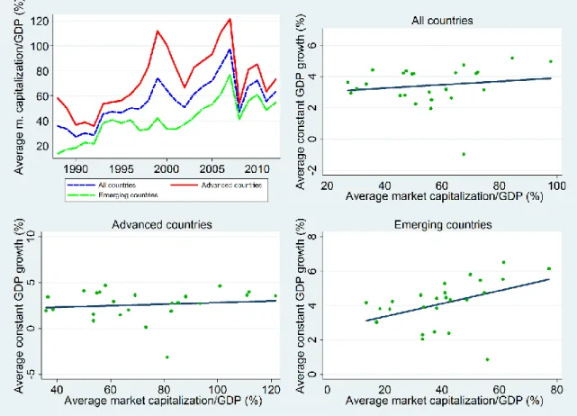
(20) Stock Markets, Banks and Economic Growth in a Context of Common Shocks and Cross-Country Dependencies. positive evolution for all samples, and that private deleveraging has occurred in recent years, particularly in advanced countries. 23 The other three plots show a negative relation between the average GDP growth and the average ratio of bank credit, for all samples. Moreover, they suggest that high levels of average banking credit might be associated with low or negative levels of average GDP growth in the case of the full sample, and that this might be explained by advanced countries. These levels coincide with those in the last two decades, as shown on the plot of the upper left.. Fig. 1. The upper left chart presents the average private credit by banks as a share of GDP (in percentages), for the time period between 1961 and 2014, the sample of all countries, and the subsamples of advanced and emerging economies. The other three graphs present the correlation of the average constant GDP growth with the average ratio of bank credit to GDP (both in percentages) for each year between 1961 and 2014, and for the three samples. We overlay a linear fit which predicts the average constant GDP growth from the average ratio of bank credit to GDP.. Fig. 2 presents the long-term characteristics of the average market capitalization of listed companies as a share of GDP, and illustrates its correlation with average GDP growth (both in percentages). The plots 23. The box plots in Fig. A4 in the online supplement coincide with this illustration.. Instituto Universitario de Análisis Económico y Social Documento de Trabajo 03/2017, 46 páginas, ISSN: 2172-7856 20.

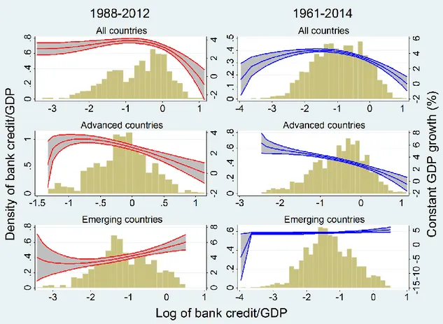
(21) Stock Markets, Banks and Economic Growth in a Context of Common Shocks and Cross-Country Dependencies. show data for all abovementioned samples, and indicate that, for all of these samples, average market capitalization has followed a positive trend over time, despite of an abrupt contraction during the recent financial crisis,24 and that it is positively correlated with GDP growth.. Fig. 2. The upper left chart presents the average market capitalization of listed companies as a share of GDP (in percentages), for the time period between 1988 and 2012, the sample of all countries, and the subsamples of advanced and emerging economies. The other three graphs present the correlation of the average constant GDP growth with the average ratio of market capitalization of listed companies to GDP (both in percentage) for each year between 1961 and 2014, and for the three samples. We overlay a linear fit which predicts the average constant GDP growth from the average ratio of market capitalization of listed companies to GDP.. Fig. 3 presents histograms of the log of the ratio of private credit by banks to GDP, and overlays fractional polynomial lines (with a 95% confidence interval) for GDP growth against the log of the ratio of private credit by banks to GDP. It includes information for all samples and the two time periods we study here. It clearly shows potential nonlinearities between both variables, as confirmed by recent studies (with thresholds between 60% and 90% for the sample of all countries, and both time frames), and strengthens the conclusions we obtain from Fig. 1, in that high levels of bank credit might be associated with lower 24. See Fig. A5 from the online supplement for similar evidence.. Instituto Universitario de Análisis Económico y Social Documento de Trabajo 03/2017, 46 páginas, ISSN: 2172-7856 21.

(22) Stock Markets, Banks and Economic Growth in a Context of Common Shocks and Cross-Country Dependencies. or negative levels of GDP growth, particularly for the full sample and the subsample of advanced economies. However, there is no graphical evidence for similar nonlinearities across the samples. In fact, Fig. A1 and Fig. A2 from the online supplement show that there are observed heterogeneities in nonlinearities for nine advanced and emerging countries and both time periods.. Fig. 3. It presents histograms of the log of the ratio of private credit by banks to GDP, and overlays fractional polynomial lines (with a 95% confidence interval) for GDP growth against the log of the ratio of private credit by banks to GDP. On the left side, plots are for a time frame from 1988 to 2012, and on the right side for a time period between 1961 and 2014. The first row of the graphs corresponds to the full sample, while the second and the third represent data for advanced and emerging economies, respectively.. The above shows that, although it might be reasonable to analyze nonlinearities in the finance-growth nexus, it should be done by addressing these heterogeneities and those which are produced by unobserved common shocks, otherwise empirical analysis might be misleading. We do not study such heterogeneous nonlinearities here because it would require large time-series data for our main financial development variables to obtain consistent estimates for the full sample and for each country.25 Thus, we leave the estimation of heterogeneous 25. Ours is not the first study to mention such data constraints, particularly for the proxy variables of stock market development (see Arcand et al., 2015).. Instituto Universitario de Análisis Económico y Social Documento de Trabajo 03/2017, 46 páginas, ISSN: 2172-7856 22.

(23) Stock Markets, Banks and Economic Growth in a Context of Common Shocks and Cross-Country Dependencies. tipping points for further research. Fig. 4 illustrates a similar analysis for GDP growth and the log of the ratio of market capitalization of listed companies to GDP. It shows that there are no thresholds beyond which larger levels of market capitalization are associated with a smaller growth of GDP, but this feature is not identical across samples and the abovementioned nine countries (see Fig. A3 from the online supplement).. Fig. 4. It presents histograms of the log of the ratio of market capitalization of listed companies to GDP, and overlays fractional polynomial lines (with a 95% confidence interval) for GDP growth against the log of the ratio of market capitalization of listed companies to GDP. Plots are for a time frame from 1988 to 2012. The first row of graphs (from the left to the right) present data for the full sample and for advanced countries, respectively; while the plot in the second row presents data for emerging economies.. This causes important problems for estimating country-specific, and even average, thresholds effects (Chudik et al., 2017); and since stock markets and banks provide complementary services (as stated in Section 2.1.), we believe that both financial development variables should have enough time series data for estimating of threshold effects.. Instituto Universitario de Análisis Económico y Social Documento de Trabajo 03/2017, 46 páginas, ISSN: 2172-7856 23.

(24) Stock Markets, Banks and Economic Growth in a Context of Common Shocks and Cross-Country Dependencies. 4. RESULTS. 4.1. Cross-Section Dependence and Unit Root Tests To study the extent of the cross-section dependence of errors caused by unobserved common shocks, we use the cross-section dependence (CD) test of Pesaran (2004, 2015) as in Chudik et al. (2017) and Eberhardt and Vollrath (2016). The implicit null hypothesis of the CD test, which is based on the average pair-wise error correlations and tested at a 5% level of significance, is a weak cross-section dependence of errors, and the alternative is a strong error cross-section dependence. 2627 In line with Chudik et al. (2017), a rejection of the null implies that such a strong error cross-section dependence might be due to unobserved common factors/shocks which are omitted or not properly accounted for. In this case, the estimates might be seriously biased and inconsistent. We also employ this test to examine the cross-section correlations of variables for the two panel data sets (the results are in Tables C9-C10 from the online supplement). We find that all the series are strongly cross-sectionally dependent in both panels, except for the one for liquid liabilities, which is weakly cross-sectionally dependent. We also carry out panel unit root tests, as in Eberhardt et al. (2013) and Eberhardt and Teal (2013), to investigate the stationarity of the variables and residuals of the static models. We employ (i), the firstgeneration panel unit root test of Maddala and Wu (1999) (for variables only); and (ii), the second-generation panel unit root test of Pesaran (2007) (for variables and residuals).28 The null hypothesis of these tests is that all the series are nonstationary and it is tested at a 5% level of significance. We examine these two tests by performing Dickey Fuller (DF) regressions, including (i) a zero to three lags augmentation for the. 26. More specifically, in line with the exponent of cross-sectional dependence, α, introduced in Bailey et al. (2016), the null hypothesis refers to the case when 0 ≤ 𝛼 < 1/2, which corresponds to different degrees of weak cross-sectional dependence, in contrast with the case when 1/2 < 𝛼 ≤ 1, which refers to different degrees of strong cross-sectional dependence.. According to Chudik et al. (2017), even though the properties of the CD test for dynamic panels that include lagged dependent and independent variables have not yet been investigated, the CD test continues to be valid in the presence of these types of variables. 28 We only use the Pesaran (2007) unit root test to examine the stationarity of residuals, since it accounts for the effect of unobserved common shocks; still, when we employ the Maddala and Wu (1999) unit root test we obtain similar results. Moreover, Pesaran et al. (2013) show that the Pesaran (2007) unit root test is exposed to size distortions if there is more than one common factor. Therefore, we suggest that further research should focus on addressing this concern. 27. Instituto Universitario de Análisis Económico y Social Documento de Trabajo 03/2017, 46 páginas, ISSN: 2172-7856 24.

(25) Stock Markets, Banks and Economic Growth in a Context of Common Shocks and Cross-Country Dependencies. panel from 1988 to 2012; and (ii), a zero to four lags augmentation for the panel from 1961 to 2014.29 From our results (found in Tables C1-C8 from the online supplement), we infer that, for the panel between 1988 and 2012, all variables in levels may be integrated of order 1 (I(1)), except for log inflation, which might be I(0), and log human capital, which is neither I(0) nor I(1). In this panel, we do not employ these variables for static models since cointegration in this case requires all variables to be I(1); 30 we nevertheless employ the log of inflation in dynamic models. Moreover, the results for the panel between 1961 and 2014 suggest that all the variables are I(1), except for log inflation, GDP growth, GDP per capita growth, and the log human capital, all of which are I(0). In the results we also provide the Root Mean Squared Error (RMSE), the number of country-time observations (NXT), and the number of countries (N) per regression.31. 4.2. Long-run effects of banking and stock market development on growth from 1988 to 2012 4.2.1. Estimates of the basic static and dynamic models Table 3 presents the results of the pooled panel estimators (POLS, 2FE, FD), and the CCEP, MG, and CCEMG estimators, according to the static specifications (4) and (5). Overall, the development of stock markets has positive, long-term statistical effects on economic growth. The effect of banking development, on the other hand, is negative and statistically significant. Turning to the diagnostics, the Pesaran (2007) unit root test suggests that the 2FE and CCEP models yield nonstationary residuals. Furthermore, the CD test shows that the MG estimator suffers from strong residual cross-section dependence. Due to these problems, we infer that the 2FE, CCEP and MG models may be misspecified, while the estimates of the POLS, FD and CCEMG specifications are consistent.. We determine the lag length for each panel by analyzing DF regressions and following information criteria such as the AIC or BIC. In addition, DF regressions of the Pesaran (2007) unit root test are augmented with crosssection averages to account for cross-sectional dependence. 30 See Engle and Granger (1987) and Breitung and Pesaran (2008). 31 We carry out our empirical analysis by employing the Stata commands written by Markus Eberhardt, such as the xtcd, xtmg and multipurt. 29. Instituto Universitario de Análisis Económico y Social Documento de Trabajo 03/2017, 46 páginas, ISSN: 2172-7856 25.

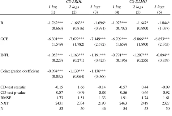
(26) Stock Markets, Banks and Economic Growth in a Context of Common Shocks and Cross-Country Dependencies. TABLE 3 Static models according to the basic specification POLS 2FE FD CCEP (1) (2) (3) (4). MG (5). CCEMG (6). B. -0.667*** -1.284*** (0.171) (0.353). -2.474** (1.200). -2.115*** (0.571). -4.122*** (0.769). -3.780*** (0.855). S. 0.480*** 1.547*** (0.133) (0.223). 1.073** (0.427). 1.977*** (0.316). 1.855*** (0.232). 2.170*** (0.279). -0.39 0.69 I(0) 3.39 1259 54. 0.20 0.84 I(1) 2.53 1313 54. 38.15 0.00 I(0) 2.63 1313 54. -0.07 0.94 I(0) 2.09 1313 54. CD-test statistic CD-test p-value Order of Integration RMSE NXT N. 0.06 0.95 I(0) 3.24 1313 54. -0.41 0.68 I(1) 2.77 1313 54. Notes: GDP growth is the dependent variable. Log domestic credit to private sector by banks to GDP (B) and log market capitalization of listed companies to GDP (S) are the independent variables. The estimates of the intercept term are omitted. Standard errors are given in parentheses. Results are reported for a period of time from 1988 to 2012. Estimators: (1) POLS: Pooled OLS, augmented with T-1 year dummies; (2) 2FE: Two-way fixed effects, augmented with T-1 year dummies and N-1 country dummies; (3) FD: First Differences, augmented with T-2 year dummies; (4) CCEP: Pooled Pesaran (2006), augmented with common country dummies and cross-section averages; (5) MG: Mean Group Pesaran and Smith (1995); (6) CCEMG: Common Correlated Effects MG Pesaran (2006), augmented with cross-section averages. White heteroskedasticity-robust standard errors are reported for models (1)(4). For models (5)-(6) we report (i), the estimates of the outlier-robust mean of parameter coefficients across groups following Hamilton (1992); and (ii), nonparametric standard errors according to Pesaran and Smith (1995) and Pesaran (2006) (the latter only for (6)). Levels of significance are represented by * 10%, ** 5% and *** 1%. Diagnostics: (evaluated at the 5% level of significance, full results of the following tests are available on request): 1) CD test: The Pesaran (2004, 2015) test, for which Ho: Weak cross-section dependence of the residuals (the test statistic as well as the p-value for each model are reported). 2) CIPS test: The Pesaran (2007) test evaluates the order of integration of the residuals where I(0): stationary, I(1): nonstationary. We include an augmentation of up to 3 lags in the Dickey Fuller regressions employed. The root mean squared error (RMSE), NXT number of country-time observations and N number of countries are also included.. The estimates of the dynamic models in Table 4 are statistically significant and agree with those presented in Table 3 in terms of the sign of the effect of the financial development variables on GDP growth. Moreover, a long-term cointegration is achieved at the 1% level in the ARDL models. While the estimates of the POLS, 2FE, CS-ARDL and CSDL are consistent, the results of the MG and DL-MG models are seriously biased and inconsistent, due to strong residual cross-section dependence. Results from Tables A1 and A2 from the online supplement show that when modelling bank and stock market development separately by employing all of the above estimators, the level of significance and sign of the estimates coincide with those of the. Instituto Universitario de Análisis Económico y Social Documento de Trabajo 03/2017, 46 páginas, ISSN: 2172-7856 26.

(27) Stock Markets, Banks and Economic Growth in a Context of Common Shocks and Cross-Country Dependencies. abovementioned results.3233 As can be seen, some of the pooled static and dynamic models provide consistent estimates even when unobserved common factors are ignored. However, further estimates, in particular those in section 4.3., suggest that we cannot fully rely on pooled specifications because they ignore potential observed countryspecific features and error cross-section dependencies, and may therefore yield inconsistent estimates. TABLE 4 Dynamic models according to the basic specification POLS 2FE MG DLMG CS-ARDL (1) (2) (3) (4) (5). CS-DLMG (6). B. -1.013*** -1.930*** (0.268) (0.441). -3.905*** (0.844). -4.317*** (0.794). -4.679*** (1.568). -4.871*** (1.638). S. 0.592*** 1.757*** (0.196) (0.299). 2.642*** (0.333). 2.583*** (0.323). 3.078*** (0.724). 3.244*** (0.621). -0.569*** -0.816*** (0.042) (0.048). -0.944*** (0.039). Cointegration coefficient. CD-test statistic CD-test p-value RMSE NXT N. -0.42 0.67 2.86 1259 54. -0.76 0.44 2.64 1259 54. 30.07 0.00 2.21 1259 54. -1.261*** (0.073) 30.23 0.00 2.30 1259 54. -1.92 0.05 0.82 1133 52. -1.59 0.11 1.25 1167 54. Notes: GDP growth is the dependent variable. Log domestic credit to private sector by banks to GDP (B) and log market capitalization of listed companies to GDP (S) are the independent variables. The estimates of the intercept term are omitted. Standard errors are given in parentheses. Results are reported for a period of time from 1988 to 2012. Long run estimates of dynamic models and cointegration coefficients of ARDL models are reported. Estimators: (1) POLS: Dynamic autoregressive distributed lagged (ARDL) Pooled OLS, augmented with T-2 year dummies; (2) 2FE: Dynamic ARDL Two-way fixed effects, augmented with T-2 year dummies and N-1 country dummies; (3) MG: Dynamic ARDL Mean Group Pesaran and Smith (1995); (4) DLMG: Distributed lagged DL Mean Group; (5) CS-ARDL: Dynamic cross-sectional ARDL Chudik and Pesaran (2015a), augmented with three lags of the cross-sectional averages of the dependent and independent variables; (6) CS-DLMG: Cross-sectional DL Chudik et al. (2016) Mean Group, augmented with three lags of the cross-sectional averages of the independent variables. Models (1), (2), (3) and (5) are represented by a Error Correction Model (ECM) and are augmented with one lag of the dependent and independent variables. Standard errors of ARDL models are computed via the Delta method. Models (4) and (6) are augmented with one lag of the independent variables. White heteroskedasticity-robust standard errors are reported for models (1) and (2). For models (3)-(6) we report (i), the estimates of the outlier-robust mean of parameter coefficients across groups following Hamilton (1992); and (ii), nonparametric standard errors according to Pesaran and Smith (1995) and Pesaran (2006) (the latter only for (5) and (6)). Levels of significance are represented by * 10%, ** 5% and *** 1%. Diagnostics: See Table 3, except for the CIPS test.. For a brief description of the results from the online supplement that complement the findings that we present here, see section A1. 33 We obtain similar findings when we model bank development separately and use data from 1988 to 2014. 32. Instituto Universitario de Análisis Económico y Social Documento de Trabajo 03/2017, 46 páginas, ISSN: 2172-7856 27.