Informa Ltd Registered in England and Wales Registered Number: 1072954 Registered office: Mortimer House, 37-41 Mortimer Street, London W1T 3JH, UK
International Journal of Computer Mathematics
Publication details, including instructions for authors and subscription information:http://www.tandfonline.com/loi/gcom20
Asymptotic behaviour of a mathematical model of
hematopoietic stem cell dynamics
M. Adimy a , O. Angulo b , J. C. López-Marcos c & M. A. López-Marcos c
a
INRIA Team Dracula, Université, Lyon 1, CNRS UMR 5208, Institut Camille Jordan, 43 blvd. du 11 novembre 1918, F-69622, Villeurbanne-Cedex, France
b
Departamento de Matemática Aplicada, ETSIT, Universidad de Valladolid, Pso. Belén 15, 47011, Valladolid, Spain
c
Departamento de Matemática Aplicada, Facultad de Ciencias, Universidad de Valladolid, Pso Belén 7, 47011, Valladolid, Spain
Accepted author version posted online: 26 Feb 2013.
To cite this article: M. Adimy , O. Angulo , J. C. López-Marcos & M. A. López-Marcos (2013): Asymptotic behaviour of a mathematical model of hematopoietic stem cell dynamics, International Journal of Computer Mathematics, DOI:10.1080/00207160.2013.778400
To link to this article: http://dx.doi.org/10.1080/00207160.2013.778400
Disclaimer: This is a version of an unedited manuscript that has been accepted for publication. As a service to authors and researchers we are providing this version of the accepted manuscript (AM). Copyediting, typesetting, and review of the resulting proof will be undertaken on this manuscript before final publication of the Version of Record (VoR). During production and pre-press, errors may be discovered which could affect the content, and all legal disclaimers that apply to the journal relate to this version also.
PLEASE SCROLL DOWN FOR ARTICLE
Full terms and conditions of use: http://www.tandfonline.com/page/terms-and-conditions
This article may be used for research, teaching, and private study purposes. Any substantial or systematic reproduction, redistribution, reselling, loan, sub-licensing, systematic supply, or distribution in any form to anyone is expressly forbidden.
A
cc
ep
te
d
M
an
us
cr
ip
t
International Journal of Computer Mathematics
Vol. 00, No. 00, January 2008, 1–11
RESEARCH ARTICLE
Asymptotic behaviour of a mathematical model of hematopoietic stem cell dynamics
M. Adimya and O. Angulob∗ and J.C. L´opez-Marcosc and M.A. L´opez-Marcosc aINRIA Team Dracula, Universit´e Lyon 1, CNRS UMR 5208, Institut Camille Jordan,
43 blvd. du 11 novembre 1918, F-69622 Villeurbanne-Cedex, France;
bDepartamento de Matem´atica Aplicada, ETSIT, Universidad de Valladolid, Pso. Bel´en
15, 47011 Valladolid, Spain;
cDepartamento de Matem´atica Aplicada, Facultad de Ciencias, Universidad de
Valladolid, Pso Bel´en 7, 47011 Valladolid, Spain
(Received 19 Oct 2012, revised 08 Jan 2013, accepted 18 Feb 2013)
We deeply researched into the asymptotic behaviour of a numerical method adapted for the solution of mathematical model of hematopoiesis which describes the dynamics of a stem cell population. We investigated the stationary solutions of the original model by their numerical approximation: we proved the existence of a numerical stationary solution that provides a good approximation to the nontrivial equilibrium solution of the problem. Also, we presented a numerical simulation which confirms this behaviour.
Keywords:Hematopoietic stem cell; Population dynamics; Age-structured model; Asymptotic analysis; Numerical integration
AMS Subject Classification: 35Q80; 35l50; 65M25; 92C37
1. Introduction
All blood cells arise from a common origin in the bone marrow, the hematopoietic stem cells (HSC). These stem cells are undifferentiated and have a high proliferative potential. They can proliferate and mature to form all types of blood cells: the red blood cells, white cells and platelets. Hematopoiesis is the term used to describe this process of production and regulation of blood cells. The HSC compartment is separated in two sub-compartments: proliferating and non-proliferating [16, 18] (also known as resting, quiescent or G0 phase). Resting cells represent the main part of the HSC population (90% of HSC are in a resting compartment [18]). Pro-liferating cells are actually in the cell cycle (G1-S-G2-M) where they are committed to divide during mitosis at the end of this phase. After division, the two newborn daughter cells enter immediately in G0-phase. A part of them remains in the HSC compartment (self-renewal) [17]. The other part can enter by differentiation into the mature cells compartment [20].
Mathematical modeling of hematopoietic stem cell dynamics has been investi-gated intensively since the 1970s (see, for example, Mackey [16]) and still interests a
O. Angulo, J.C. L´opez-Marcos, M.A. L´opez-Marcos were supported in part by the Ministerio de Ciencia e Innovaci´on (Spain), project MTM2011-25238.
∗Corresponding author. Email:[email protected]
ISSN: 0020-7160 print/ISSN 1029-0265 online c
2008 Taylor & Francis DOI: 0020716YYxxxxxxxx http://www.informaworld.com
A
cc
ep
te
d
M
an
us
cr
ip
t
lot of researchers. This interest is greatly motivated, on one hand, by medical appli-cations and, on the other hand, by the biological phenomena (such as oscillations, bifurcations, traveling waves, or chaos) observed in these models (Mackey [16], Adimyet al. [4–6]).Blood cells die and must be replaced continuously. In the normal conditions, the body must maintain a constant blood volume to function properly. Then, the hematopoiesis regulates its internal environment to maintain a stable population of blood cells (homeostasis). It is believed that several hematological diseases are due to some abnormalities in the feedback loops between different compartments of hematopoietic populations [5, 6, 13, 16]. These disorders are considered as major suspects in causing destabilization of the homeostasis.
In this work, we consider a model of HSC dynamics with age-dependent coeffi-cients which was proposed in [4]. It is comprised by a nonlinear partial differential system of equations that represents a balance law,
rt+ra=−(δ(a) +β(a, R(t)))r, 0< a, t >0,
pt+pa=−(γ(a) +g(a))p, 0< a < τ, t >0, (1)
a non local boundary condition, that means the way in which cells regenerate,
r(0, t) = 2R0τg(a)p(a, t)da, t >0,
p(0, t) =R∞
0 β(a, R(t))r(a, t)da, t >0,
(2)
and a set of initial conditions
r(a,0) =r0(a), 0≤a,
p(a,0) =p0(a), 0≤a < τ. (3)
The independent variables a and t are, respectively, spent age in each phase and time. The dependent variablesr(a, t) andp(a, t) are densities of resting and prolif-erating HSC, respectively. The age has no limit for resting cell, whereas a maximal division ageτ is used for proliferating ones. Since we assume here that τ is finite, all proliferating cells that did not die must divide before they reach it (see [14]). All the vital functions depend on age, which is the internal variable:δ(a) is the differ-entiation rate of resting cells (also, it could count some necrosis) andγ(a) andg(a) are the apoptosis and division rate of proliferating cells, respectively. The transi-tion rate from resting phase to proliferating compartment,β, depends on the age and the total number of resting cellsR(t) =R∞
0 r(a, t)da,t >0. In our model the
positive equilibrium is the homeostasis of the hematopoietic stem cell population. This age-structured model (1)–(3) was previously studied by Adimyet al.[4]. The authors proved the existence and uniqueness of solutions to this problem. They also investigated the existence of stationary solutions with the contribution of the conditions that a nontrivial stationary solution must satisfy. However, the stability of such equilibrium was not theoretically investigated. The authors introduced a numerical method adapted to (1)–(3) to show such stability.
Models such as the one considered above cannot be solved analytically and re-quire numerical integration to obtain an approximation of the solutions. In [1, 2], we can find a review of the numerical schemes proposed to solve models of phys-iologically structured populations, which are compared with regards to accuracy, efficiency, generality, mathematical methodology and qualitative behavior depend-ing on the compatibility conditions between initial and boundary data of the prob-lems. On the other hand, modern numerical methods have been successfully applied to physiologically structured models to replicate available field and/or laboratory
A
cc
ep
te
d
M
an
us
cr
ip
t
data, for a variety of different systems [3, 7–11, 15]. All these works indicate that structured population models and numerical simulations are valid tools to investi-gate systems such as the one under consideration here. Besides, new techniques for the numerical solution of more general nonlocal boundary problems than (1)-(3) has been recently introduced in [12].The numerical method used in [4] was very helpful to investigate the dynamics of the solutions of problem (1)-(3). In different numerical tests, the authors observed the existence of an asymptotically stable steady state. This represents, from a medical point of view, the situation of normal hematopoiesis (homeostasis). The unstable nontrivial steady state produces long-period oscillations which can be related to observations of some periodical hematological diseases. However, the theoretical study of this numerical procedure was not performed in our previous work [4]. This is the aim of this work.
In section 2, we introduce the theoretical results developed in [4] about sys-tem (1)–(3). In section 3, we present the numerical method. We show the existence of the nontrivial numerical steady state provided by the method, and we analyze the convergence of the numerical steady state to the theoretical one in section 4. Finally, in section 5, we numerically illustrate our results.
2. Theoretical Properties of the Model
In this section, we describe some properties of the solutions of (1)–(3). In this way, we introduce the following assumptions related to the vital rates (see [4] for more details).
(A1) For R∈R+, the function β satisfies 0≤β(·, R)≤β+ a.e., decreasing with respect toR on [0,+∞) and limR→+∞β(·, R) = 0, a.e. in [0,+∞). (A2) There is an increasing functionC: [0,+∞)→[0,+∞) such that, if 0≤
R1 ≤M and 0≤R2 ≤M then:kβ(·, R1)−β(·, R2)k∞≤C(M)|R1−R2|. (A3) Function δ satisfies 0≤δ≤δ+ a.e.in [0,+∞).
(A4) Function γ satisfies 0≤γ ≤γ+ a.e. in [0, τ). (A5) Functiong is nonnegative, belongs toL1
loc[0, τ) and Rτ
0 g(a)da= +∞. Under (A1)-(A5), the existence of a unique local solution of system (1)–(3) can be proved via a fixed point argument (see [19]). On the other hand, regularity, positivity and global existence of this solution depend on the initial conditions and some criteria on the parameters of the model. With respect to stationary solutions,
r(a, t) = ϕ(a), a > 0, and p(a, t) = ψ(a), 0 < a < τ, we observe that the trivial
equilibrium (i.e. (ϕ, ψ) ≡ (0,0)) always exists. On the other hand (see [4] for a more detailed discussion), we can characterize another stationary solution in the following way. We denote by Φ the total number of resting cells at the steady state, Φ =R0∞ϕ(a)da. Then a nontrivial steady state can be written as
ϕ(a) = R+∞Φ Λ (a,Φ) 0 Λ (σ,Φ)dσ
,0≤a; ψ(a) = ΦL(a)
2K R0+∞Λ (σ,Φ)dσ,0≤a < τ; (4)
withL(a) = exp−R0a(γ(s) +g(s))ds, Λ (a,Φ) = exp−R0a(δ(σ) +β(σ,Φ))dσ,
K=R0τg(a) exp−R0a(γ(σ) +g(σ))dσ da, and Φ is just a solution of the equation
2K
Z +∞
0
β(a,Φ) Λ (a,Φ)da= 1. (5)
A
cc
ep
te
d
M
an
us
cr
ip
t
Therefore, if we define the net growth rate of the population at the constant size asH(Φ) := 2KR0+∞β(a,Φ) Λ (a,Φ)da, from (5), the existence of such nontrivial equilibrium, is just associated to the existence of solutions of equationH(Φ) = 1. So, under (A1)-(A5) we have the following resultProposition 2.1 System (1)–(2) has exactly one nontrivial stationary solution if
H(0)>1. Otherwise, no nontrivial stationary solution exists.
3. Numerical method
In this section, we describe a method which integrates numerically the nonlin-ear system (1)–(3) along the characteristic curves. Taking into account that the problem is defined over an unbounded age interval, for numerical purposes we in-troduce a maximum individual ageAmax for resting cells (Amax will be considered enough large to assure that after this maximum age, the density r vanishes, and
soτ < Amax).
The numerical method that we propose integrates the model along the char-acteristic curves by means of a discretization of an integral representation of the solutions of the model. We introduce an age grid in which we stateτ as a node. To this end, given a positive integerJ, we define the step sizek=τ /J and denoting byJ∗
= [Amax/k], we introduce a uniform partition on the interval [0, Amax], given by aj =j k, 0 ≤ j ≤ J∗ (note that aJ = τ). We will integrate the problem in a fixed time interval [0, T], so we define the discrete time levels,tn=n k, 0≤n≤N, whereN = [T /k].
The values Un
j, 0≤j ≤J ∗
, and Vn
j , 0≤j≤J, for each 0 ≤n ≤N, represent numerical approximations to r(aj, tn) and p(aj, tn), respectively (the subscript j refers to the grid pointaj and the superscriptnto the time leveltn); we also denote the discrete approximations as vectors Un, Vn, 0 ≤ n ≤ N, with components
Un
j, 0 ≤ j ≤ J ∗
, and Vn
j , 0 ≤ j ≤ J, respectively. The notations Ik(W) and
I∗
k(W) represent the open second order quadrature rules Ik(W) = PJ−1
j=1 000
k Wj,
forW= (W0, . . . , WJ), andIk∗(W) =
PJ∗−1 j=1
000
k Wj, forW= (W0, . . . , WJ∗), that
will be used to approach the nonlocal terms (the notation P000 indicates that the first and last term are multiplied by 32).
Given approximations U0 ∈ RJ∗+1
, V0 ∈ RJ+1 of the initial conditions in (3), the numerical method is defined from the following general recursion that pro-vides the numerical approximation at the time leveln+ 1, (Un+1,Vn+1), from the approximations at the time leveln, (Un,Vn):
Uj+1n+1 =Ujn exp
−k
2
βnj +βn+1j+1− Z k
0
δ(aj+σ)dσ
,0≤j ≤J∗
−1, (6)
Vj+1n+1 =Vjn exp
−
Z k
0
(γ(aj+σ) +g(aj+σ))dσ
, 0≤j≤J −1. (7)
The discretization of the boundary conditions provides the numerical boundary values that complete the description of this time step,
U0n+1 = 2Ik(g· Vn+1), (8)
V0n+1 =I∗
k(βn+1· Un+1), (9) 0 ≤ n ≤ N −1. We denote as g and βn, 1 ≤ n ≤ N, vectors with components
A
cc
ep
te
d
M
an
us
cr
ip
t
g(aj), 0≤j≤J, andβ(aj, Ik∗(Un)), 0≤j≤J∗, respectively. The productsg·Vn and βn· Un, in (8)-(9), represent the componentwise product of the vectors g,
Vn, and βn, Un, respectively. Note, that for sake of simplicity only the nonlocal dependent function β has been discretized. Depending on the expressions of the other age-dependent functions, the required integrals may be exactly obtained or numerically computed. In any case, taking into account that these values do not change with time, they can be obtained before the numerical method starts. An analysis of convergence as in [11] can be applicable for this numerical procedure.
4. Asymptotic Behavior of the Numerical Scheme
As in the model, the trivial solution is a steady state of the numerical method. Now, if we look for a nontrivial equilibrium solution of (6)-(9), it is easy to see that such solution (U,V) satisfies
Uj+1=Uj exp
−k
2 βj+βj+1
− Z k
0
δ(aj+σ)dσ
, 0≤j≤J∗
−1,
Vj+1=Vj exp
−
Z k
0
(γ(aj +σ) +g(aj +σ))dσ
, 0≤j ≤J−1,
U0 = 2Ik(g· V),
V0 =Ik∗(β· U).
Nowβ represents the vector with componentsβj =β(aj, Ik∗(U)), 0≤j ≤J ∗
−1. Next, we can describe the equilibrium solution of the numerical method in terms of the numerical total population of resting cells, and such total population as a solution of a transcendental equation only involving the parameters of the problem. So, denoting by Sk = Ik∗(U), then a nontrivial numerical steady state can be written as
Uj =
SkΛk(aj, Sk) Θ∗
k(Sk)
,0≤j ≤J∗
; Vj =
SkL(aj) 2KkΘ∗k(Sk)
,0≤j≤J, (10)
with Λk(aj, Sk) = exp
−Pji=000
kβi−Raj
0 δ(σ)dσ
, Kk =
PJ−1 j=1
000
k g(aj) exp −R0aj(γ(σ) +g(σ))dσ
, Θk(Sk) =
PJ∗−1 j=1
000
kβjΛk(aj, Sk),
Θ∗
k(Sk) = PJ
∗−1 j=1
000
kΛk(aj, Sk), (where the notation P00 indicates that the first and the last term are multiplied by 12). Now Sk is just a solution of the equation
2KkΘk(Sk) = 1, (11) discrete counterpart of (5). Associated to this equation we define the numerical growth rate of the population at the constant size asHk(Sk) := 2KkΘk(Sk).
Now, we want to show that the equilibrium solution of (6)-(9) is just an ap-propriate approximation of the equilibrium solution of (1)-(2) as the step size k
tends to zero. In order to obtain this convergence result, we consider the following steps. First, note that the inclusion of Amax for the numerical method could be interpreted as a modification of the original model by truncation of the age inter-val. Therefore, we will show the convergence of the steady state solution of this truncated model to the steady state of (1)-(2) as Amax goes to infinity. Then we
A
cc
ep
te
d
M
an
us
cr
ip
t
conclude the convergence of the numerical equilibrium solution to the equilibrium of the truncated system ask goes to zero.Therefore, we consider the introduction of Amax for resting cells as a change of the original model by means of a truncation version of the system over [0, Amax]. So we introduce
rt+ra=−(δ(a) +β(a, R(t)))r, 0< a < Amax, t >0,
pt+pa=−(γ(a) +g(a))p, 0< a < τ, t >0, (12)
(
r(0, t) = 2R0τg(a)p(a, t)da, t >0,
p(0, t) =RAmax
0 β(a, R(t))r(a, t)da, t >0,
(13)
r(a, t) =r0(a), 0≤a≤Amax,
p(a, t) =p0(a), 0≤a≤τ. (14)
Now, the total number of resting cells is defined byR(t) =RAmax
0 r(a, t)da,t >0.
By means of the same procedure than the one used to obtain the equilibrium solution of (1)-(2), we can characterize the equilibrium solution of (12)-(13) in terms of the total number of resting cells at the steady state. So, denoting by ( ¯ϕ(a),ψ¯(a)) a nontrivial steady state of the truncated model, and ¯Φ =RAmax
0 ϕ¯(a)da, its total number of resting cells, we can write
¯
ϕ(a) = Φ Λ¯ a,Φ¯
RAmax
0 Λ σ,Φ¯
dσ,0≤a < Amax; ¯ψ(a) =
¯ ΦL(a) 2K RAmax
0 Λ σ,Φ¯
dσ,0≤a < τ,
(15) where ¯Φ is just a solution of the equation
2K
Z Amax
0
β a,Φ¯Λ a,Φ¯da= 1, (16)
truncated version of (5). Again, we define the net growth rate of the population at the constant size ¯Φ asHmax Φ¯:= 2K R0Amaxβ a,Φ¯Λ a,Φ¯da. The following result states that the equilibrium solution of (12)-(13) converges to the nontrivial stationary solution of (1)-(2) exponentially withAmax, by assuming the following regularity condition
(A6) The function x → β(a, x) is continously differentiable on [0,∞), for
a≥0, andβx(·, x) belongs toL1 forx≥0. Whereβx describes the derivative with respect to the second argument,
Theorem 4.1 Let (A1)-(A6) be satisfied. IfH(0)>1, there existsA∗
maxsuch that
if Amax > A∗max, (12)-(13) has exactly one nontrivial stationary solution. In such
case, letΦand Φ¯ denote the unique positive solutions of (5) and (16), respectively, and let be definedϕ and ψ by (4) and ϕ¯ and ψ¯ by (15).Then, there exist positive constantsαi, i= 1,2,3, such that,
|Φ−Φ¯|=O(e−α1Amax
), (17)
|ϕ(a)−ϕ¯(a)|=O(e−α2Amax
), a∈[0, Amax], (18) |ψ(a)−ψ¯(a)|=O(e−α3Amax
), a∈[0, Amax]. (19)
Otherwise, no nontrivial stationary solution of (12)-(13) exists.
Proof: First we prove the existence and uniqueness of solutions of the
A
cc
ep
te
d
M
an
us
cr
ip
t
tion (16). As H(0) > 1 and limAmax→∞Hmax(0) = H(0), we can find A∗ max such that if Amax > A∗max then Hmax(0) > 1. Now, we consider the function
ξ(x) = 1−Hmax(x), related to the transcendental equation (16) that defines ¯Φ (i.e.,ξ( ¯Φ) = 0). Note that forAmax> A∗max,ξ(0)<0 andξ
0
(x)>0 (because func-tionHmax(x) is decreasing in (0,+∞)). Now, from the assumptions imposed to the vital functions, and using similar arguments used in the proof of Proposition 2.1 (see [4]) for the original model, we can conclude that, limx→+∞ξ(x) = 1. So, ¯Φ is the unique positive root ofξ, and ¯Φ<Φ because ξ(Φ)>0.
By means of the mean value theorem, (A1) and (A6) and the smoothness prop-erties of vital functions, there existsΦe ∈( ¯Φ,Φ) such that
|Φ¯−Φ| ≤C
R+∞
Amaxβ(a,Φ) Λ (a,Φ)da
ΛAmax,Φe R0Amax
−βx
a,Φeda
≤C e−RAmax
0 β(a,Φ)da≤C e−α1Amax,
so (17) holds. On the other hand, if a ∈ [0, Amax], then, (4) and (15), the mean value theorem, (A3), (A1) and (A6), allow us to arrive at
|ϕ(a)−ϕ¯(a)| ≤ |ϕ(0)−ϕ¯(0)|+C
Z a
0
β(s,Φ)ds−
Z a
0
β s,Φ¯ds
≤ |ϕ(0)−ϕ¯(0)|+C Φ−Φ¯. (20) Now, after some computations we arrive at
|ϕ(0)−ϕ¯(0)| ≤C|Φ¯−Φ|+C
Z +∞
Amax
Λ (a,Φ)da+C
Z Amax
0
Λ a,Φ¯da− Z +∞
0
Λ (a,Φ)da
, (21) Therefore, by means of (A3), (A1) and (A6), and using (21) in (20) we can con-clude (18). Finally, ifa∈[0, Amax], (4) and (15) and properties (A4)-(A5) produce
|ψ(a)−ψ¯(a)| ≤ |ψ(0)−ψ¯(0)|= 1
2K |ϕ(0)−ψ¯(0)|
that, by means of (18) and properties (A3), (A1) allows us to obtain (19).
By means of similar arguments than in Theorem 4.1, and using the convergence properties of the quadrature rules that are included in the description of the numer-ical scheme, we can arrive to the following result which shows that the equilibrium solution of the numerical method (6)-(9) converges to the equilibrium solution of the truncated problem as k tends to zero. More precisely, the convergence is of second order.
Theorem 4.2 Let be the vital functions δ, β, g and γ sufficiently smooth. If
Hmax(0)>1then, fork >0enough small, (11) has a unique solution. In such case,
letΦ¯ andSkdenote the unique positive solutions of (16) and (11), respectively, and
let be defined ϕ¯ and ψ¯ by (15) and U andV by (10). Then, as k→0
|Φ¯−Sk|=O(k2), (22) |ϕ¯(aj)−Uj|=O(k2), 0≤j≤J∗, (23) |ψ¯(aj)−Vj|=O(k2), 0≤j≤J. (24)
Proof: Consider the function ξk(x) = 1−Hk(x), related to the transcendental equation (11) that definesSk (i.e. ξk(Sk) = 0). Note that, fork sufficiently small,
A
cc
ep
te
d
M
an
us
cr
ip
t
due to the regularity properties of functionβand the error bound of the quadrature rule, (ξk)0(x) = −2KkΘ0k(x) > 0 on (0,+∞); limx→∞ξk(x) = 0 and Hk(0) =Hmax(0) +O(k2), soSk is the unique positive root of ξk.
By means of the mean value theorem applied to the functionξ−1
k on the interval defined byξk( ¯Φ) andξk(Sk), there exists Φ in this interval such thate
|Φ¯ −Sk|= ξ−1
k 0
(ξk(Φ))e
ξk( ¯Φ)−ξk(Sk) =
2 (K−Kk)
Z Amax
0
β(a,Φ)Λ¯ a,Φ¯da−2Kk
Z Amax
0
β(a,Φ)Λ¯ a,Φ¯da−Θk( ¯Φ)
2KkΘ0k(Φ)e
.
The regularity properties of the vital functions, and the error bounds of the quadra-ture rule allow us to obtain that
|K−Kk| ≤C k2,
Z Amax
0
β(a,Φ)Λ¯ a,Φ¯da−Θk( ¯Φ)
≤C k2.
By means of these inequalities, and thatK > 0 and bounded, we conclude (22). Next, if 0≤j≤J∗
, (15) and (10) allows us to have |ϕ¯(aj)−Uj| ≤ |ϕ¯(a0)−U0|Λ aj,Φ¯
+U0
Λ aj,Φ¯
−Λk(aj, Sk)
, (25) the smoothness properties of the vital functions and the error bounds of the quadra-ture rules allow us to get
Λ aj,Φ¯
−Λk(aj, Sk)
≤C k2. (26) On the other hand, due to the boundedness and regularity properties of the vital functions, (22) and the error bounds of the quadrature rules, we arrive at
|ϕ¯(a0)−U0| ≤C
Φ¯ −Sk+C
Z Amax
0
Λ a,Φ¯da−Θ∗ k(Sk)
≤C k2. (27) Then, we obtain (23) by using (26)-(27) in (25). Finally, using (15) and (10), and the positivity of the vital functions, we have
|ψ¯(aj)−Vj| ≤ |ψ¯(a0)−V0|. (28) And, with the boundedness of data functions, we get
|ψ¯(a0)−V0| ≤C
Φ¯ −Sk+C
Z Amax
0
Λ a,Φ¯da−Θ∗ k(Sk)
+
Z Amax
0
β a,Φ¯Λ a,Φ¯da−Θk(Sk)
(29) and by means of the same smoothness arguments applied to (29) we arrive at
|ψ¯(a0)−V0| ≤C k2,
A
cc
ep
te
d
M
an
us
cr
ip
t
which substituted in (28) allow us to have (24).From Theorem 4.1 and Theorem 4.2, we can conclude that the equilibrium solu-tion of the numerical method, given by (10), is close to the theoretical equilibrium solution, given by (4), by takingAmaxlarge enough andksufficiently small. On the other hand, we can conclude the same convergence result for the total populations.
5. Numerical experiments
In this section, we will integrate numerically (1)–(3) by means of the numerical method introduced in Section 3. We are going to show how much the numerical stationary state approaches the theoretical one. The initial conditions are given by functions r0(a) = ν(Amax−a) andp0(a) = Γ(τ −a), whereν and Γ are fixed constants, chosen in a suitable form in order to satisfy the compatibility condition between the initial and boundary conditions. We also use the following values (see Adimy et al. [4]) τ = 7, δ(a) = 0.05, γ(a) = 0.2, g(a) = τ−1a. The transition rate functionβ is taken as
β(a, R) =βe0(a)
θn
θn+Rn,
with θ = 1.62 ×10⁸. We have considered two kinds of functions βe
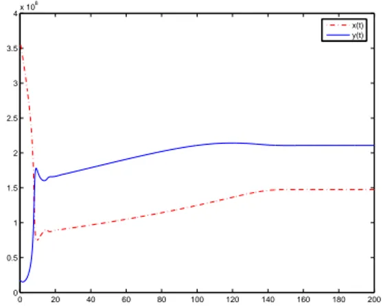
0(a) but, in all the cases, the maximum of βe0(a) is β0 = 1.77. In the first test problem, we use βe0(a) = β0(1−e−α a), with α = 1 and n = 6, which satisfies H(0) > 1. In this case, the theoretical study of the model (1)–(3) (see [4]) predicts a positive steady state. It describes, from a medical point of view, a normal hematopoiesis (homeostasis). We show in Fig. 1 the results obtained with our numerical method. We present the evolution with time of total populations of resting and proliferating cells. We observe that the numerical solution is attracted towards a positive stable equilibrium. Due to the convergence results (Theorem 4.1 and Theorem 4.2), such asymptotically stable equilibrium provides an accurate numerical approximation of the theoretical steady state predicted in the analysis of the model. So, the numerical observations carried out provide relevant information about the dynamics of the solutions of the model.
0 20 40 60 80 100 120 140 160 180 200 0
0.5 1 1.5 2 2.5 3 3.5 4x 10
8
x(t) y(t)
Figure 1. Evolution with time of resting population (straight line) and proliferating population (dashed line), forα= 1 andn= 6.
In the second test problem we have takenn= 2 andβe0(a) =β0, because we are able to obtain the exact value of the theoretical steady state Φ. So we compare this value with the numerical results in order to show its convergence. We have
A
cc
ep
te
d
M
an
us
cr
ip
t
used Amax = 400, and we have computed the difference between the theoretical and numerical steady states for different values of the step size. Then, the quantityrk= log
|Φ−Sk|/|Φ−Sk
2|
/log 2, provides numerically the order of convergence to the theoretical steady state. The results in table 1 shows the predicted second order of convergence.
k rk
1e-2 2.045 5e-3 2.003 2.5e-3 1.997 1.25e-3 1.997
Table 1. Numerical order of convergence of the numerical steady state to the theoretical one.
6. Conclusions
We considered a problem that describes the evolution of an hematopoietic stem cell population. We took into account cell age dependence of coefficients. We an-alyzed the asymptotic behaviour of a new numerical method proposed ad hoc to solve the model. We obtained that when the model presents a nontrivial stationary solution, the numerical method also does, and the numerical stationary solution converges to the original one. We presented numerical experiments which corrobo-rate the theoretical results. First, the numerical method was able to approach the nontrivial steady state in a case in which it is not possible to obtain theoretically such equilibrium. On the other hand, we showed that this convergence is of second order.
References
[1] L.M. Abia, O. Angulo, and J.C. L´opez-Marcos,Size-structured population dynamics models and their numerical solutions, Discrete Contin. Dyn. Syst. Ser. B 4 (2004), pp. 1203–1222.
[2] L.M. Abia, O. Angulo, and J.C. L´opez-Marcos,Age-structured population models and their numerical solution, Ecol. Model. 188 (2005), pp. 112–136.
[3] L.M. Abia, O. Angulo, J.C. L´opez-Marcos, and M.A. L´opez-Marcos,Numerical study on the prolif-eration cells fraction of a tumour cord model, Math. Computer Model. 52 (2010) pp. 992-998. [4] M. Adimy, O. Angulo, F. Crauste, and J.C. L´opez-Marcos,Numerical integration of a mathematical
model of hematopoietic stem cell dynamics, Comput. & Math. Appl. 55 (2008), pp. 337–366. [5] M. Adimy, F. Crauste, and S. Ruan,A mathematical study of the hematopoiesis process with
appli-cations to chronic myelogenous leukemia, SIAM J. Appl. Math. 65 (2005), pp. 1328–1352.
[6] M. Adimy, F. Crauste, and S. Ruan, Stability and Hopf bifurcation in a mathematical model of pluripotent stem cell dynamics, Nonlinear Anal. Real World Appl. 6 (2005), pp. 651–670.
[7] O. Angulo, J.C. L´opez-Marcos and M.A. Bees,Mass Structured Systems with Boundary Delay: Os-cillations and the Effect of Selective Predation, J. Nonlinear Sci. 22 (2012), pp. 961-984.
[8] O. Angulo, J.C. L´opez-Marcos and M.A. L´opez-Marcos,Numerical approximation of singular asymp-totic states for a size-structured population model with a dynamical resource, Math. Computer Model. 54 (2011), pp. 1693-1698.
[9] O. Angulo, J.C. L´opez-Marcos, M.A. L´opez-Marcos, and J. Mart´ınez-Rodr´ıguez,Numerical analysis of an open marine population model with spaced-limited recruitment, Math. Computer Model. 52 (2010) pp. 1037-1044.
[10] O. Angulo, J.C. L´opez-Marcos, M.A. L´opez-Marcos, and J. Mart´ınez-Rodr´ıguez, Numerical inves-tigation of the recruitment process in open marine population models, J. Stat. Mech. Theory Exp. (2011) P01003, doi:10.1088/1742-5468/2011/01/P01003.
[11] O. Angulo, J.C. L´opez-Marcos, M.A. L´opez-Marcos, and F.A. Milner,A numerical method for non-linear age-structured population models with finite maximum age, J. Math. Anal. Appl., 361 (2010), pp. 150-160.
[12] B. Bialecki, G. Fairweather, and J.C. L´opez-Marcos,Orthogonal spline collocation for quasilinear problems with nonlocal boundary conditions, Adv. App. Math. Mech. (2012)accepted.
[13] C. Foley and M.C. Mackey,Dynamic hematological disease: a review, J. Math. Biol. 58 (2009), pp. 285-322.
A
cc
ep
te
d
M
an
us
cr
ip
t
[14] M. Iannelli, Mathematical Theory of Age-Structured Population Dynamics, Applied MathematicsMonographs, C.N.R., Giardini Editori e Stampatori, Pisa, 1994.
[15] Y. Kocak, and A. Yildirim,An efficient algorithm for solving nonlinear age-structured population models by combining homotopy perturbation and Pad´e techniques, Int. J. Comput. Math. 88 (2011), pp. 491-500.
[16] M.C. Mackey,Unified hypothesis of the origin of aplastic anaemia and periodic hematopoiesis, Blood 51 (1978), pp. 941-956.
[17] B.R. Smith,Regulation of hematopoiesis, Yale J. Biol. Med. 63 (5) (1990) 371-380.
[18] W. Vainchenker,H´ematopo¨ı`ese et facteurs de croissance, Encycl. Med. Chir., Hematologie, 13000, 1991, M85.
[19] G.F. Webb,Theory of nonlinear age-dependent population dynamics, Monographs and Textbooks in Pure and Applied Mathematics 89, Marcel Dekker Inc., New-York, 1985.
[20] I.L. Weissman, I.L.,Stem cells: units of development, units of regeneration, and units in evolution, Cell 100 (2002), pp. 157-168.