The Intertemporal Approach to the Current Account: Evidence from
Argentina
Diego N. Moccero
The Intertemporal Approach to the Current
Account: Evidence from Argentina
Diego N. Moccero
[email protected]
PSE (Paris School of Economics) - ENS
Abstract
In this paper, an intertemporal model is used to analyze the current account and test whether it accounts for the evolution of the Argentinean current account over the period extending from 1855 to 2002. The in-tertemporal model presented here takes into account several sources of external shocks for small economies such as a change of the real interest rate and the real exchange rate. Evidence shows that the intertemporal model does not pass the statistical tests and does not explain the
Argen-tinean experience. More specifically, if the Argentinean current account
was to behave as the model predicts, one would observe the opposite move-ment to that observed for the actual current account. Our main conjecture about the weak performance of the model is related to i) the fact that one of its most important assumption is violated for some part of the period under consideration (1931 - 1989); and ii) that the balance of payments’ crises and stop and go cycles may have altered the relation between the variables suggested by the model. To cope with this problem, we have estimated a model for the period 1885-1930 (a period with relatively high capital mobility and with neither currency crises nor stop and go cycles) and found some evidence in favour of this result. A general conclusion to be drawn is that, in contrast to other Latin American countries, an intertemporal current account model can not appropriately account for the dynamics of the current account of Argentina, even thought there is some evidence in favour of the model for the period 1885-1930.
1
Introduction
we can distinguish the “old” or traditional view, which studies the specific de-terminants of trade andfinancialflows, and the “new” or modern view (called the intertemporal approach to the current account), that highlights the impor-tance of saving-investment decisions taken by forward-looking optimizing agents in the determination of the internationalflow of commodities andfinancial cap-ital. In the simpler intertemporal models, a country’s current account surplus should be equal to the present value of expected future declines in output, net of investment and government purchases (called net output). In these papers there is no room for a variable real interest rate and for the real exchange rate. More recent papers expand earlier models precisely by considering the role played by those variables in the determination of the current account.
For the case of Argentina the few papers that exist on the subject use mostly the “old view” to analyze the current account. In particular, Musalem (1984 and 1985) estimates econometrically an equation for the determination of the trade balance including as explanatory variables the real exchange rate and the international interest rate. On the other hand, Wynne (1997) makes an analysis of the determinants of aggregate savings and its impact on growth. In this context, the author studies the sustainability of the Argentinean current account during the 90s.
In this paper we use an intertemporal model to the current account and test it both formally and informally to see whether it can account for the evolution of the Argentinean current account during the period 1885 - 2002. In particular, we know that the current account of Argentina has exhibited largefluctuations through time. Particularly, during the last part of the XIXth century and the beginning of the XXth century (Belle Epoque), the country had access to the internationalfinancial market that allowed it tofinance important current ac-count deficits (of approximately 6% of the GDP per year during 1885-1931). Since then, the international environment has changed drastically. Firstly with the occurrence of the big crises of the 30s and secondly with the Second World War. The international trade has slumped and protectionary policies were ap-plied world wide. The country could not maintain the huge current account imbalances of the past and we observed an almost equilibrated current account until the beginning of the 90s (-0,1% of GDP). Since 1990 and as a consequence of the rise in external funds available to developing countries, Argentina could once again run important current account imbalances of the order of 3.4% of GDP during the period 1992-2001. A good question would then be to know whether an intertemporal current account model may account for the dynamics in the current account of Argentina since the last part of the XIXth century. In accordance with the simpler intertemporal theory, the periods 1885-1930 and 1991-2002 should have been periods in which agents anticipated a rising net output while in the period 1931-1990 agents should have expected a decline in net income. Given that the end of the XIXth and the beginning of the XXth century were very affluent times and that the opposite case applies for the pe-riod 1931-1991, it seems that in principle the theory should track the long run evolution of the current account in Argentina reasonable well.
ap-proach by enhancing the theoretical and empirical elements that favored its creation (Section 2). Section 3 briefly exposes the theory of “present value mod-els” which underlies all the empirical work made on the intertemporal approach. This section also makes a revision of the applied literature, an important obser-vation is that the majority of the papers applied a “simple” version of the current account model where only the future evolution of the “net output” (gross do-mestic product less investment and government expenditures) was relevant. An important extension of these models that also considers a variable interest rate and the real exchange rate in the determination of the current account is pre-sented in Section 4 (The Theoretical Model). The precise econometric method used to test the theory is presented in Section 5. This is just an application to the current account of the concepts and methods developed in Section 3. The construction of the data needed to test this theory for the case of Argentina is presented in Section 6. Various sources of data were combined tofinally build the long time series needed to test the theory (the working-age population, the real exchange rate, nominal interest rates and so on for the period 1885 - 2002). Section 7 exposes the empirical results,first checking that the time series have the necessary properties to be included in the model and estimating a Vector Auto Regression Model (VAR). We then combine some key parameters of the theory (the intertemporal discount factor, the share of non tradables on total private consumption, etc.) and the results from the VAR to obtain the formal and informal results for the validity of this model for the case of Argentina. Section 8 concludes.
2
The Intertemporal Approach and its Origins
Intertemporal analysis of the current account balance became common in the early 1980s when researchers begun to explore the implications of modeling the current account based on assumptions of representative individuals that made forecasts of the relevant variables in a rational expectations context. Buiter (1981) and Sachs (1981a and 1981b), Obstfeld (1982), Greenwood (1983) and Svensson and Razin (1983) have developed such models highlighting these fea-tures. This was the result from both theoretical advances and from economic events at the international level (Obstfeld and Rogoff, 1994).
On the one side, the Lucas’s Critique of econometric policy evaluation was one important theoretical motivation for an intertemporal approach. His insis-tence on grounding policy analysis in the actual forward-looking decision rules of economic agents suggested that open-economy models might yield more reli-able policy conclusions if demand and supply functions were derived from the optimization problem of households and firms rather than specified to match reduced-form estimates based on ad hoc econometric specifications.
pat-terns of current account adjustments by industrialized and developing countries raised the inherently intertemporal problem of characterizing the optimal re-sponse to external shocks. Similarly, the explosion in bank lending to developing countries after thefirst oil shock sparked fears that borrowers’ external debt lev-els might become unsustainable. The need to evaluate developing-country debt levels again led naturally to the notion of an intertemporally optimal current-account deficit.
One might of course wonder whether this theory that was created as a re-sponse to precise international events during a certain period of time could be applied to examine other cases and circumstances. Even if not of the same nature and with some qualifications, some of the characteristics of thefinancial markets turmoil in the 70s were also seen during the 90s and even, over the last part of the nineteenth century. In particular, for the last part of the nine-teenth century we know that it was a period of very high capital mobility, with resourcesflowing from the Old World (mainly England) to the New world (see Williamson et al., 1994; Obstfeld et al., 2002; and Taylor, 2002). As for the 70s and 90s we know that the proportion of private to official capital inflows to less developed countries has grown substantially, the international money market has expanded dramatically, and capital controls have been liberalized in many developing countries (for an analysis of the 70s period see Sachs, 1981b). As a consequence, most Latin American countries exhibited current account imbal-ances. This was also the case for the biggest economy in the world (the US) which raised again some concerns over the sustainability of these imbalances (see Mann, 2002).
3
How to Test the Theory
To test this theory, “present value” models are used by recent papers. In these type of studies, one variable is written as a linear function of the present dis-counted value of other variables.1 These analysis rely heavily on the modern
theory of time series and on vector auto regressive models. One of their most important virtues is that they make use of the theoretical model’s structure to derive testable hypothesis.
Thefirst articles that applied this technique over current account data ap-peared in the early 90s. In these simple versions of the intertemporal model the objective was to expand the idea of Campbell (1987) that consumers “save for a rainy day”, to an open economy. In particular in the earlier literature, a coun-try’s current account surplus was equal to the present value of expected future declines in output, net of investment and government purchases (called directly the net output). The analogy to household savings is instructive: households save when they expect their future labor income to decline. The key element that is being introduced by using this type of test is how one proxies for
pri-1In formal terms a present value model for two variablesy
t andYt states that the last
variable can be written as: Yt=P∞i=0δiEtyt+i; whereδis the discount factor,Et denotes
vate agents’ expectations of future values of the relevant variables. The basic insight is that as long as the information set used by the econometrician does not contain all the information available to private agents, then past values of the current account should contain information useful in constructing estimates of agents’ expectations of future values of the relevant variables (net output in these early models and interest rates and the real exchange rate in the more modern models, as we will see later). Another important feature of these mod-els is that the international real interest rate is considered to be constant and there is no room for non tradable goods.
The pioneering paper on the subject is the one by Sheffrin and Woo (1990a). The authors study the case of Belgium, Canada, Denmark and the UK for the period 1955-1985. They found evidence in favor of the theory only in the case of Belgium. Later on, other case studies have appeared: Otto (1992) considered the case of US and Canada using quarterly data for the period 1950:1 to 1988:4. For both countries, the formal restrictions implied by the present-value relationship for the current account are strongly rejected, finding only some “informal” evidence in favor for the US case. Ghosh (1995) studied the case of Japan, Germany, the US, Canada and the UK using quarterly data for the period 1960 : 1 - 1988 : 4. He concludes that the model performs extremely well in characterizing the direction and turning points of the current accounts of the countries studied even if the theory can not be rejected only in the case of US. More recently, McDermott et al. (1999) wrote a paper for France using quarterly data for the period 1970: 1 to 1996:4finding that the model explains thefluctuations of the current account balance fairly well, even for a period during which France experienced large external shocks and there were restrictions on overseas capital transactions.
One thing to note is that papers for developing economies are by far less common. For Latin America and to our knowledge, there are only two studies that applied the simple version of the model: one for Colombia and the other for Peru. For thefirst country, Suarez Parra (1998) tests this simpler version of the intertemporal model using annual data over the period 1950 - 1996 and for the second economy, Arena and Tuesta (1999) do the same thing using annual data for the period 1960 - 1996. For both countries the intertemporal model seems to track quite well the effective movement in the actual current account. A somewhat general finding in all these articles is that the actual current account is in fact more volatile than the “theoretical” current account, except in the case of the US.2As noted by Bergin and Sheffrin (2000), this is surprising
since the assumptions of the theory seem to be more appropriate for small open economies than for big ones. This result naturally leads to the idea that there were some missing variables not included in the model that should have been considered to explain the current account.
A likely explanation already advanced by Sheffrin and Woo (1990a) but not developed, is that small economies may be affected strongly by external
2
shocks not passing through changes in net output -a factor not considered in the simple version of the model. To explain the current account behavior of small economies it may be important not only to consider shocks to domestic output but also shocks arising in the world in general. These external shocks will generally affect the small economy via movements in the interest rates and exchange rates. Ten years later, Bergin and Sheffrin (2000) developed and constructed a model that precisely incorporated in the model, a moving interest rate and the real exchange rate, following a proposal by Dornbusch (1983). The idea was that an anticipated raise in the relative price of internationally traded goods can raise the cost of borrowing from the rest of the world when interest is paid in units of these goods. As a result, changes in the real exchange rate can induce substitution in consumption between periods, and thus can have intertemporal effects on a country’s current account similar to those of changes in the interest rate. In addition to these intertemporal effects, exchange rate changes of course can also have more standardintratemporaleffects by inducing substitution between internationally-traded goods and nontraded goods at some point in time. The authors tested the model for Australia, Canada and the UK and concluded that the incorporation of these variables may help explain the evolution of the current account in the case of the twofirst countries over the simpler intertemporal models used in earlier tests. This model was also tested for Chile using quarterly data from 1960:1 to 1999:4, concluding that with the inclusion of both a variable real interest rate and the expected appreciation of the exchange rate, the performance of the model improves a lot over the case where these variables were not included (Landeau, 2002).
It is considered that this constitutes an important improvement to the in-tertemporal theory since it takes into account two other sources of possible external shocks which may in principle be very important for small developing economies. This is the case since as it is widely known, interest rates and the exchange rate are more volatile in developing countries than in developed ones. In what follows we will present this model in detail and test its functioning for the case of Argentina.
4
The Theoretical Model
As aforementioned, we consider the model developed by Bergin and Sheffrin (2000) in which a small country produces traded and nontraded goods. The country can borrow and lend with the rest of the world at a time-varying real interest rate. The representative household solves an intertemporal maximiza-tion problem, choosing a path of consumpmaximiza-tion and debt that maximizes the expected discounted lifetime utility:
maxEt +∞
X
s=t
βs−tU(CT s, CNs)
whereU(CT t, CN t) =
1 1−σ
¡
CT ta CN t1−a¢1−σ
σ >0, σ6= 1, 0< a <1
Etdenotes expectations conditional on agents’ timetinformation set.
Con-sumption of the traded good is denotedCT t, and consumption of the nontraded
good isCN t. Yt denotes the value of current output, It is investment
expen-diture, andGt is government spending on goods and services, all measured in
terms of traded goods. The relative price of home nontraded goods in terms of traded goods is denoted Pt. The stock of external assets at the beginning of
the period is denotedBt. Finally,rtis the net world real interest rate in terms
of traded goods, which may vary over time. The lefthand side of this budget constraint may be interpreted as the current account. We may express total consumption expenditure in terms of traded goods asCt=CT t+PtCNt.
From thefirst-order conditions for this problem we can derive the following optimal consumption profile (see Appendix A):
1 =Et
"
β(1 +rt+1)
µ Ct
Ct+1
¶σµ
Pt
Pt+1
¶(1−σ)(1−a)#
(2)
Assuming joint log normality and constant variances and covariances, con-dition (2) may be written in logs as:
Et∆ct+1=γEtr∗t+1 (3)
where γ = 1/σ is the intertemporal elasticity of substitution andr∗ t+1 is a
consumption-based real interest rate defined by:
rt∗+1=rt+1+ ∙1
−γ
γ (1−a) ¸
∆pt+1+ constant term
We also define∆ct+1= lnCt+1−lnCtand∆pt+1= lnPt+1−lnPt. For the
world real interest rate (defined in terms of traded goods) we use the approxima-tion: ln (1 +rt+1)≈rt+1. The constant term at the end of the expression will
drop out of the empirical model when we later demean the consumption-based real interest rate. See Appendix B for a derivation of these equations.
This condition characterizes how the optimal consumption profile is infl u-enced by the consumption-based real interest rate, rt∗, which reflects both the interest rate rt and the change in the relative price of nontraded goods, pt.
increase in the conventional real interest rate, rt, makes current consumption
more expensive in terms of future consumption foregone, and induces substitu-tion toward future consumpsubstitu-tion.
A similar intertemporal effect can result from a change in the relative price of nontraded goods. If the price of traded goods is temporarily low and ex-pected to raise, then the future repayment of a loan in traded goods has a higher cost in terms of the consumption bundle than in terms of traded goods alone. Thus the consumption-based interest rate r∗ raises above the
conven-tional interest rate r, and lowers the current total consumption expenditure. In addition to this intertemporal substitution, a change in the relative price of nontraded goods also induces intratemporal substitution. Again if the price of traded goods is temporarily low relative to nontraded goods, households will substitute toward traded goods by the intratemporal elasticity, which is unity under a Cobb-Douglas specification. This intratemporal effect will be domi-nated by the intertemporal effect if the intertemporal elasticity (γ) is greater than unity.
The representative agent optimization problem above entails an intertempo-ral budget constraint (equation (1)) that may be rewritten as:
Bt=N Ot−Ct+ (1 +rt)Bt−1
where we define net output as follows: N Ot = Yt−It−Gt. Net output
is random and the source of uncertainty in the model. Define also Rt,S as the
market discount factor betweenS andt so that (forS > t):
Rt,S =
1
S
Q
j=t+1
(1 +rj)
with the convention thatRt,t= 1 Summing and discounting over all periods
of the infinite horizon, and imposing the following transversality condition:
lim
T→+∞Rt,TBT = 0
we may write an intertemporal budget constraint:
+∞
X
s=0
Rt,t+sCt+s= +∞
X
s=0
Rt,t+sN Ot+s+B 0
t (4)
whereBt0 is the initial net foreign assets. We log linearise this intertemporal budget constraint to get:
− +∞
X
s=1
βs
∙∆no t+s
Ω −∆ct+s+
µ 1− 1
Ω
¶ rt+s
¸ = 1
Ωnot−ct+
µ 1− 1
Ω
¶ b0t+
where lower case letters represent the logs of upper case counterparts, except in the case of the world real interest rate, where we use again the approximation that ln (1 +rt)≈rt.HereΩis a constant grater than one,Ω= 1 +BΨ, whereB
is the steady state value of net foreign assets andΨis the steady state value of the present value of net output. Next, take expectations of this equation and combine it with the log-linearized Euler equation (3) to write:
−Et +∞
X
s=1
βs
∙∆no t+s
Ω −γr
∗ t+s+
µ 1−Ω1
¶ rt+s
¸ =not
Ω −ct+
µ 1−Ω1
¶ b0t+
+ constant term
The right hand side of this equation is similar to the definition of the current account (CAt = N Ot−Ct+rtBt−1), except that its components are in log
terms and there appearsΩand a constant term in it. We label this transformed representation of the current account asCA∗t. We will follow the convention of choosing the steady state around which we linearize to be the one in which net foreign assets are zero (B = 0). In this case, Ω = 1 and the condition above may be written:
CA∗t =−Et +∞
X
s=1
βs¡∆not+s−γrt∗+s
¢
(6)
where CA∗
t ≡not−ct and where we neglected the constant term since in
the empirical model we will demean all the variables.3 See Appendix C for a
derivation of the intertemporal budget constraint and its log-linearization. This condition says that if net output is expected to fall, the current account will rise as the representative household smooths consumption. But the condition also says that aside from any change in domestic output, a rise in the consumption-based interest rate will raise the current account by inducing the representative household to lower consumption below its smoothed level. Then, the agent may also be willing to “unsmooth” consumption because of changes in the consump-tion based real interest rate. For comparison, we also test two simpler versions of the intertemporal model. In the first one, the consumption-based interest rate is assumed to be constant, and consequently only thefirst of the two effects described above will occur. This amounts to testing a condition similar to (6) above, where the second term in the brackets is not present. The second version is one in which we only allow for a variable real interest rate, the real exchange rate being constant in the expression of the consumption based real interest rate. The objective in thefirst case is to see whether an expanded model can improve upon the simpler versions developed in the early literature and in the second one, if any, to try to determine the source of this improvement.
3
5
The Econometric Method
To test the restriction that the current account depends on expected future values of net output and the consumption based interest rate, we mustfirst have proxies for these two sets of expected values. The simplest approach would be to project every single variable (the net output, the real interest rate and the exchange rate appreciation) on past values of itself. As noted by Ghosh (1995), this is unlikely to be adequate since individual agents will in general have a much richer information set on which base their expectations. Nowadays, the standard procedure for generating expectations of the net output and the consumption based real interest rate is to project these variables forward on the basis of past data using a VAR framework in which the past values of all of the series intervene in the expectation formation. As noted in all of the papers already mentioned on the subject, this is equivalent to regarding conditional expectations as equivalent to linear projections on the information set. In turn, as noted in Campbell and Shiller (1988), one possibility would be to consider the expression∆not+s−γrt∗+s
as a single variable from which we make expectations, in which case we would have to estimate just a two variable VAR. As Bergin and Sheffrin (2000) do, another option is to consider∆not+sandrt∗+sas separate variables and estimate
a three variable VAR. Instead, the option that we follow here is to consider the change in net output, the real interest rateandthe appreciation rate of the real exchange rate as separate variables. The advantage over the other possibilities is that in this fashion, one can judge the relative importance of every variable, if any, on the current account If the model performs well, we would then be able to see which of the three variables is more important in determining the evolution of the current account.
In order to do that, we rewrite equation (6) using the expression for the consumption based real interest rate that takes into account that r∗
t+s is a
function ofrt+sand∆pt+s:
CA∗t =−Et +∞
X
s=1
βs[∆not+s−γrt+s−(1−γ)(1−a)∆pt+s] (7)
As will be said in the next section, as Argentina suffered from exchange rate controls in their international transactions during some periods of time, it is convenient to split the appreciation of the real exchange rate (∆pt+s) into
two components. One component corresponds to the appreciation of the real exchange rate calculated using a “commercial” exchange rate and the other, to one corresponding to a “market” exchange rate. Thefirst one corresponds to a regulated exchange rate used for exports and imports while the second one is the “free market” exchange rate determined in the black or free market.4 We
will then call∆pC
t+sthe appreciation of the commercial real exchange rate and
∆pM
t+s the appreciation of the market real exchange rate. We are now able to
rewrite equation (7) as (wherebis a weighting parameter):
CA∗t =−Et +∞
X
s=1
βs£∆not+s−γrt+s−(1−γ)(1−a)
£ b∆pC
t+s+ (1−b)∆pMt+s
¤¤
(8) Under the null hypothesis of this last equation, the current account itself should incorporate all of the interest rate, devaluation rate and net output changes specified in that equation.5 This leads us to estimate a five variable
VAR to represent consumers’ forecasts:
⎡ ⎢ ⎢ ⎢ ⎢ ⎣ ∆no CA∗ r
∆pC
∆pM ⎤ ⎥ ⎥ ⎥ ⎥ ⎦ t = ⎡ ⎢ ⎢ ⎢ ⎢ ⎣
a11 a12 a13 a14
a21 a22 a23 a24
a31 a32 a33 a34
a41 a42 a43 a44
a51 a52 a53 a54 ⎤ ⎥ ⎥ ⎥ ⎥ ⎦ ⎡ ⎢ ⎢ ⎢ ⎢ ⎣ ∆no CA∗ r
∆pC
∆pM ⎤ ⎥ ⎥ ⎥ ⎥ ⎦
t−1
+ ⎡ ⎢ ⎢ ⎢ ⎢ ⎣ u1 u2 u3 u4 u5 ⎤ ⎥ ⎥ ⎥ ⎥ ⎦ t (9)
Or written more compactly: zt=Azt−1+ut, whereE(zt+s) =Aszt. This
may easily be generalized for higher orders of VAR. A test of the simpler model that holds interest and devaluation rates constant would involve a VAR that omits the third, fourth andfifth equations and the third, fourth and fifth vari-ables. Of course, a model that considers the appreciation rate of the real ex-change rate to be constant is one that omits the forth andfifth equations and variables in the VAR system.
Using (9), the restrictions on the current account in (8) can be expressed as:
CA∗t =h0z
t=−
+∞
X
s=1
βs[g0
1−γg20 −(1−γ)(1−a)g03]Aszt (10)
whereg0
1= [1 0 0 0 0],g02= [0 0 1 0 0],g30 = [0 0 0 b1−b], andh0 = [0 1 0 0 0]
(again this can be generalized for a larger number of lags). If the VAR is stationary, it is possible to write (10) as:
CA∗t =h−[g0
1−γg20 −(1−γ)(1−a)g30]βA(I−βA)−1
i zt
With the estimated parameters of the VAR and some values for the param-etersβ,γ, aandbit is possible to find the estimated optimal current account:
∧
CA∗t =k0z
t
where:
k0=−[g0
1−γg02−(1−γ)(1−a)g03]βAb
³
I−βAb´−1
5Note that what matters for the determination of the current account is the agent’s
whereAbis the matrix of estimated parameters from the VAR. This expres-sion gives a model prediction of the current account variable consistent with the VAR and the restrictions of the intertemporal theory. Note that k0z
t is
not a forecast of the current account in the conventional sense, but rather a representation of the model’s restrictions (Bergin and Sheffrin, 2000).
In addition, if the restrictions of the theory were consistent with the data, such that CA∧∗t = CA∗t except for an innovation, then the vector k0 should equal [0 1 0 0 0]. This implies that the model may then be tested statisti-cally by using the delta method to calculate a χ2 statistic for the hypothesis
that k0 = [0 1 0 0 0]. If we write the estimated vector of VAR coefficients as π, the estimated variance-covariance matrix of these coefficients as V, and the vector of deviations of the estimated system from the theoretical model as ek (the difference between the actual k and the hypothesized value), then e
k0¡(∂k/∂π)V(∂k/∂π)0¢−1ekwill be distributed chi-squared with degrees of free-dom equal to the number of restrictions (the number of elements ofek, five in this case).6
6
Data Construction
In this section we proceed to construct the series that we will use to test the model. We had to use annual data since the National Institute of Statistics did not report quarterly data for private consumption before 1993. In any case, this is not problematic at all since this model of the current account determination seems to be more a statement of longer-run tendencies than of short run dynamics (Sheffrin and Woo, 1990b). We had to combine lots of sources of information to build the relevant series for the period 1885 - 2002, as will be seen below.
6
To see what the expressions ofV and ∂π∂k look like, let’s consider a two variable VAR
with only one lag :
µ
x1t
x2t
=
µ
a1 b1
a2 b2
¶ µ
x1t−1
x2t−1
¶ + µ 1t 1t 
.If we call the vector of
estimated parameters of the VARπ0=£ a1 b1 a2 b2 ¤,then, the estimated variance
-covariance matrix of these coefficients is given by :V =
⎡ ⎢ ⎢ ⎣
σa1a1 σa1b1 σa1a2 σa1b2
σb1a1 σb1b1 σb1a2 σb1b2
σa2a1 σa2b1 σa2a2 σa2b2
σb2a1 σb2b1 σb2a2 σb2b2
⎤ ⎥ ⎥ ⎦.
This matrix is estimated asΣ⊗(Z0Z)−1
,whereΣis the 2x2 variance - covariance matrix of the residuals andZis the matrix
⎡ ⎢ ⎣
x11 x21
.
.. ...
x1T−1 x2T−1
⎤ ⎥ ⎦.
The estimated k−vector will, in this case, be a 1x2 vector where each component is a function of the parameters in the VAR (and, of course, of the other parameters -β, γ,etc.) :
k0=£ k1(a1, b1, a2, b2) k2(a1, b1, a2, b2) ¤.Then, the expression ∂k
∂π will be a 2x4 matrix
of the form : ∂k∂π =
" ∂k1
6.1
Population and Working-age Population
All the models of the intertemporal approach to the current account express the net output and the current account in per capita terms (using total population) with the explicit goal to mimic the theoretical assumption of a representative agent. In our case, the representative agent is a person of working age and not a person in the general population . This difference may have an effect on the dynamic of the variables since in the long run the working-age population may have a different dynamic than that of the total population.
The total population for the period 1980 - 2002 was taken from CEPAL (2002). To construct the series for the period 1914 - 1979, we applied the “re-gression” method using data from Maddison (1995). That is, we ran a regres-sion in logs (natural logarithms) for the period of superposition of data (1980 - 1994) and then employed the coefficient resulting from the regression and the data from Maddison to extend CEPAL’s data overt the past.7
The data for the years that go from 1885 to 1913 was constructed using the method of “the rate of variation”. More precisely, we took the variations for the data from V´azquez-Presedo (1971) and applied them to the data previously constructed.
The population composition by age was elaborated using data from V´azquez-Presedo (1971), V´azquez-V´azquez-Presedo (1976) and the National Institute of Statistics and Censuses of Argentina (INDEC). From thefirst author we got the compo-sition by ages for the years 1869, 1895 and 1914 (which correspond to thefirst, second and third National Census). From the second author we got information for the years 1915, 1920, 1925, 1930, 1935 and 1940 (statistics published by the Oficina de Migraciones). Finally, from INDEC we also got quinquennial data for the period 1950 - 2005. Using this data we calculated the share of people between 15 and 60 years in total population (considered to be our measure of population in working age). Then, the missing values (the years for which we did not have information) were replaced with the linear interpolation between the observed values.
Finally, combining the series for total population and the share of people of working age, we constructed the series for the working - age population.
6.2
The Real Exchange Rate
The real exchange rate for the period 1900 - 1993 corresponds to that of Wino-grad and V´eganzon`es (1997) and is measured in australes (the national currency before the peso) of 1985. As was said before, we will use two series of the real exchange rate constructed by these authors since Argentina faced exchange rate
7Suppose thaty
tis a series that goes toT andxtis a series that starts inHwithH < T.
The objective is to extendytto the future, using the values ofxtfort > T.Then, we just run
a simple regression of the form ln(yt) =α+βln(xt) +εtfort∈[H, T]. For the periodT+ 1
the estimated value of (the log of)yT+1will be ln(byT+1) =αb+bβln(xT+1) +bεT, which may
be rewritten as ln(byT+1) =βb[ln(xT+1)−ln(xT)] + ln(yT). Then, for anys >1,we’ll have
controls in their international transactions beginning in the 1930s and lasting until the beginning of the 1990s. One corresponds to a commercial real ex-change rate, created using the regulated nominal exex-change rate for exports and imports. The other is a “free market” real exchange rate, using the black or free exchange rate. Of course, these series do coincide when there are no exchange rate controls (until the 30s and since the 90s). To extend these series over the past, we used the method of the “rate of variations” since we did not have a superposition period to run a regression. In order to do that, we constructed a multilateral real exchange rate for the period 1885 - 1900 as a weighted aver-age of the bilateral exchange rates between Argentina and some countries with which Argentina held strong commercial relationships. The main partners of Argentina during the last twenty years of the nineteenth century were Germany, England, United States, France and Belgium. In spite of that, we only consid-ered the threefirst countries since we did not have enough information about France and Belgium.
For every year, we used as weights, the share of each country’s trade (exports to that country and imports from that country) over the total trade with the three countries. The series of the origin of imports and the destination of exports were taken from V´azquez-Presedo (1971). The real bilateral exchange rate with every country was calculated as: BRER=N ER∗W P I∗/W P I; whereBRER is the bilateral real exchange rate,N ERis the nominal exchange rate between both countries (national currency per unit of foreign currency), W P I∗ is the
wholesale price index of the foreign country, andW P I is the wholesale price index for the home country.
In computing the bilateral exchange rates the following information was used :
Price index of Argentina and nominal exchange rate (per U.S. dollar): we used the wholesale price index and the nominal exchange rate (pesos per US dollar) presented in Della Paolera and Taylor (2003). The base for the price index is 1885 = 100.
Price index of USA: we constructed the annual wholesale price index as an average of monthly values. The source is the NBER Macrohistory Data Base. The base for the price index is 1885 = 100.
Price index of England and Nominal exchange rate between the peso and the sterling pound: We constructed the annual wholesale price index as an average of monthly values. The source was the NBER Macrohistory Data Base. The base for the price index was 1885 = 100. For the nominal exchange rate, we used a monthly series of the exchange rate between the sterling pound and the US dollar. We calculated the annual exchange rate as an average of the monthly values. Then, we used the nominal exchange rate between the peso and the US dollar to construct the exchange rate between the peso and the sterling pound.
For the period 1994 - 2002 we used the “regression method” to construct the real exchange rate. In particular, we ran a regression for the overlapping period 1980 - 1993 between the two real exchange rates of Winograd and V´eganzon`es (1997) and that calculated for the Center of International Economics (Ministry of Foreign Relationships, Argentina). This is a multilateral real exchange rate calculated using the wholesale price indexes of the countries and following the methodology presented in Ott (1997). We then used the coefficient from this regression and the data from the Center of International Economics to extend the series to 2002 as explained in an earlier footnote.
Using these series we constructed the appreciation of the commercial and market real exchange rate,first by taking the inverse of the real exchange rates, then taking their natural logarithm and finally, taking the difference with the preceding value of the variable (remember that∆pt+1= lnPt+1−lnPt).
6.3
The Wholesale Price Index
In constructing the wholesale price index we made use of three series. First of all, we used the wholesale price index published by Della Paolera and Taylor (2003) for the period 1885 - 1900. The second one was the series by Winograd and V´eganzon`es (1997) that was used to extend the later series for the years 1901 - 1993. And the last one was the one by the National Institute of Statistics and Censuses of Argentina (INDEC), from which we calculated the index for the last period 1994 - 2002. We applied the “rate of variations” method to construct the final index since we found no differences in the evolution of the series during the overlapping periods.
6.4
Nominal and Real Interest Rates
As we have already mentioned, the simpler intertemporal current account model considers a constant interest rate which was generallyfixed between 2% and 6% (Sheffrin and Woo, 1990a; Ghosh, 1995; Suarez Parra, 1998, McDermott et al., 1999). On the other hand, since the real interest rate in the model considered here is not heldfixed, the question then arises of how to construct an interna-tional real interest rate to conduct the analysis The tradiinterna-tional view consists of building an ex-ante interest rate following the method of Barro and Sala i Martin (1990). This method consists of collecting data on nominal interest rates and inflation (calculated from the consumer price index) for the G-7 economies. The expected inflation is calculated as a forecast using an ARMA model. The nominal interest rate in each country is then adjusted by inflation expectations to compute an ex-ante real interest rate. An average real interest rate is then computed using time-varying weights for each country based on its share of GDP in the G-7 total. We do not follow this procedure since in our view it does not seem to be applicable to a case like Argentina, that will usually pay a by far greater rate if it has access to the internationalfinancial market and will display far more volatility than the G-7 rate. Unfortunately, a series does not exist for the cost of capital in the internationalfinancial market for a country like Argentina. In such an event, even if it is not entirely satisfactory, we pre-fer to use an internal interest rate to the alternative of using an international interest rate as stated above.8
The nominal interest rate that we consider here is an average of a passive and active rate. The nominal active and passive rates for the period 1900 - 1993 are those presented in Winograd and V´eganzon`es (1997). For the period 1885 - 1899 we made use of the series of Della Paolera and Taylor (2001) which is respectively taken from Cortes Conde (1998). This corresponds to the implicit yield on an internal government bond (fondos p´ublicos nacionales). To extend the series by Winograd and V´eganzon`es (1997) to the years 1994 - 2002 we applied the “regression method” to our own calculations of these rates for the overlapping interval 1991 - 1993. Our active rate corresponds to an average of an active rate of the Banco Naci´on (tasa de descuento de documentos) and that of loans granted between localfinancial institutions (the source of this data is the Central Bank of Argentina). On the other hand, our passive rate is an average of the deposit rate measured by the IMF (2003) and that measured by the Central Bank of Argentina (interest rates on ordinary saving account deposits and time deposits). We then used the wholesale price index to obtain the real ex - post interest rate using the formula: rt= (1 +it)PPt+1t −1, where rt is the real interest rate between periodt andt+ 1,itis the nominal interest
rate between periodtandt+ 1 andPtis the price index for periodt.
8Surprisingly, even for the case of a small economy like Chile, Landeau (2002) follows the
6.5
Consumption and Net Output
To construct the series for consumption and net output wefirst took the data for the nominal National Accounts presented in IEERAL (1986) for the period 1914 - 1980. The net output was calculated as the gross domestic product less investment and public expenditures. We then extended these series over the future using data from INDEC. In particular, we used the nominal National Accounts (methodology 1986) to construct the net output and add it to the later using the rate of variation method for the period 1981 - 1993. The same procedure was repeated to construct the consumption variable. The source for this data was INDEC (1993).
An equal thing was done with the nominal National Accounts (methodology 1993) for the period 1994 - 2002 for both consumption and net output (the source of the data is the web page of the Direction of National Accounts, INDEC).
To extend the series over the past (1885 - 1913), we used information from Taylor (1997), V´azquez-Presedo (1971) and IEERAL (1986). From the first author we got the nominal GDP, nominal investment and the nominal total consumption (private plus public consumption). To be able to split total con-sumption into private and public concon-sumption wefirst took the share of public consumption of total consumption for the year 1914 calculated from IEERAL (1986) and applied it to the data from Taylor (1997). Then, we used the evolu-tion of the expenditures of the federal government provided by V´azquez-Presedo (1971) to reconstruct the evolution over the past for the public consumption. Note that by doing that, we neglected the evolution of the public expenditures of the local governments, which are included in the National Accounts. This didn’t seem to be a problem since by that time the local governments represented only 16% of the total public expenditures (federal plus provincial governments). See Porto (2003) on this subject. The private consumption was then obtained as the difference between total and public consumption. Finally, we were already able to compute the net output and to chain both series using again, the method of the rate of variation. Once with the series of nominal net output and consump-tion in hand, we used the wholesale price index to make the conversion into australes of 1985 and we expressed them in terms of the population in working age.
Using the series for net output and consumption, we calculated the modified current account as CA∗
t ≡ not−ct and using net output we calculated the
change in net output as∆not=not−not−1.The series for net output, private
7
Empirical Results
7.1
Checking the Stationarity of the Series
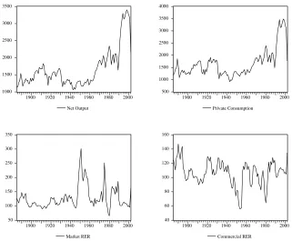
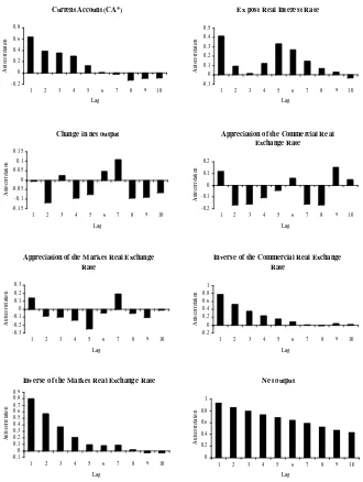
Before estimating the VAR model, we have to check that the variables that appear in it are stationary (the change in net output, the current account, the real interest rate and the appreciation of the real exchange rates). In order to do this, wefirst look at the correlograms of the series which are presented in Figure 3. Note that we included in Figure 3, not only the variables just mentioned, but also the levels of net output and of the inverse of the commercial and market exchange rate. Testing the stationarity of these series is a very important step. This is so because the estimation of a VAR such as the one presented before, for variables that are integrated of order one and cointegrated, would result in the loss of very valuable information. A more appropriate representation would in this case be a Vector Error Correction Model.9 Surprisingly, in the paper that first presented the model used here (Bergin and Sheffrin, 2000) and in later applications (Landeau, 2002) this point is not even mentioned. Observing Figure 3, we see that the only correlogram that shows a strong persistence is the one for the log of net output. This would be initial evidence that all of the series but the log of net output are stationary, because the correlogram for non-stationary variables shows a slow linear decay, while that of a stationary variable decays exponentially towards zero. To see whether this is the case we must then proceed to more formal tests.
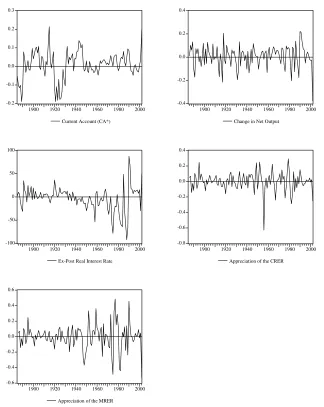
In particular, we tested for the presence of unit roots in the series using the Elliott-Rothenberg-Stock methodology. We chose this test because it is the most powerful; it is more capable of discerning a near unit root from a unit root. We proceeded as follows: first, the series that presented a trend were detrended and those that did not have a trend were demeaned to remove the deterministic components of the series.10 Based on a visual inspection of Figures 1 and 2, we demeaned the current account, the change in net output, the ex-post real interest rate, the appreciation rate of the market and commercial real exchange rate and the levels of the commercial and market real exchange rate. On the other hand, the net output was detrended. The next step consists of performing an ADF test to the series without constant or time trend, as explained in Salanie (1999).11 In order to choose the lags to be included in the ADF test we computed
the Schwarz information criteria (SIC) for every variable and up to 5 lags which seems very reasonable for annual data. We chose two lags for the test for the
9
The idea is that a principal feature of cointegrated variables is that their time paths are influenced by the extent of any deviation from long-run equilibrium. After all, if the system is to return to the long run equilibrium, the movements of the variables must respond to the magnitude of the disequilibrium. As such, when variables are cointegrated their appropiate representation is a vector error correction and not just a VAR in differences. Estimating just a VAR model would entails in this case a misspecification error.
10
Note that the terms “demeaned” and “detrended” are not used here in the conventional sense. See Salanie (1999) for a detailed explanation of this procedure.
11Remember that an ADF test without constant or time trend for any variablex
tis a test
of the form4xt =αxt−1+Ppi=1βi4xt−i+εt where we test whether the coefficientα is
current account and only one for the other variables. We cannot reject the null hypothesis that the series contain a unit root only for the level of the net output. For the rest of the variables we can reject at 5% (for the current account) and at 1% (in the other cases) that the series contain a unit root in favor of the alternative that the series are stationary.
However, before these results are accepted, it is necessary to determine whether the error terms from the estimated equations satisfy the assumptions of the Dickey-Fuller test. In particular, we tested for autocorrelation using the Breusch-Godfrey LM test statistic (that regress the residuals on the original regressors and lagged residuals) and for autoregressive conditional heteroskedas-ticity using the ARCH LM test (that regress the squared residuals on a constant and lagged squared residuals). We performed both tests starting with 5 lags and then reducing the number of lags to 4, 3, 2 and 1,finding no evidence of auto-correlation in every variable and for any lag (see Table 1). The same table shows that heteroskedasticity is a problem for some of the regressions. This is the case for the ex-post real interest rate, the appreciation of the market real exchange rate, the inverse of the market real exchange rate and the net output, where we can reject the null hypothesis of absence of conditional heteroskedasticity.
Following Trehan and Walsh (1991) we will also test for unit roots using the Phillips - Perron (PP) test for the variables that present conditional het-eroskedasticity in the residuals of the ADF regressions.12 Even if this test is less powerful than the ERS test, we will apply it to the ex-post real interest rate, the appreciation of the market real exchange rate, the inverse of the market real exchange rate and the net output because this test is robust to the presence of conditional heteroskedasticity in the error terms. To make the results com-parable with those of the ERS test, we first demeaned the series that did not not have a time trend. This was the case for the ex-post real interest rate, the appreciation rate of the market real exchange rate and the inverse of the market real exchange rate. As with the ERS test, for these series we would like to reject the null hypothesis that the series contain a unit root (this is, they are a random walk without drift) against the alternative in which they are stationary around zero. The PP test is then performed without a constant term or time trend invoking the Newey-West automatic truncation lag selection, which is four for every variable.13 The results show that we can reject the null hypothesis that
the series have a unit root in favor of the alternative for all of the variables at the 1% significance level. For the log of the net output, we computed the PP test with a constant but not a time trend, so that under the null, the series is a random walk with drift. Again, we invoked the Newey-West automatic truncation lag selection, which is again four,finding that we cannot reject the presence of a unit root.
We can then conclude that the variables to be included in the VAR are sta-tionary and that the level of the commercial and market real exchange rates are
12
Their study concerns the sustainability of the US federal Buget and the US current account during the second half of the twentieth century.
13This selection is based solely on the number of observations used in the test regression
also stationary and so, they can not be cointegrated with the net output. We then have that the appreciation rate of both real exchange rates are overdiff er-enced. We will have to take this result into account in the following section at the moment of estimating the VAR system.
7.2
Estimation of the VAR System
In this section we present the methodology used to estimate the VAR model and the residual’s analysis. To estimate the VAR we first demeaned all the variables to be included in it. We will work with the demeaned variables, since our model restricts only the dynamic interrelation between the variables but not their mean values. Then, the redefinition of variables as deviations from means enables us to drop the constant terms present in the VAR model. The variables that are included in the VAR and that were demeaned are the change in net output, the current account, the ex-post real interest rate and the appreciation rate of the commercial and market real exchange rate. We also demeaned the levels of the inverse of the commercial and market real exchange rates which are also included in the system since they are already stationary in levels. These variables will be included in the system with a two period lag.14
The next step in the estimation of the system consists of choosing an appro-priate lag length for the VAR. The criterion that we will use here consists of choosing the most parsimonious VAR which has multivariate white noise errors. In particular, we sequentially computed VARs of the order 5 to 1, and checked at each time whether their residuals were white noises in the multivariate sense.15
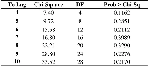
Once we do that, we choose the smallest VAR (the most parsimonious) for which the residuals are white noise. To test for multivariate white noise in the errors we apply the Portmanteau test for orders that goes fromp+ 1 to 10,wherepis the order of the VAR.16When estimating thefive VARs, we found that residuals
were white noise in the multivariate sense for the VAR with one, two and four
14To see why this is the case, consider an univariate time seriesy
t, and suppose that we
are willing to write its first difference as a function of their past differences. In order to do so start by rewriting the stochastic process using evident notation asφ(L)yt= t.After
some calculations we can easily show that the process can be rewritten as (1−φ∗(L))4yt= t−φ(1)yt−1.For expositional porposes, suppose that (1−φ∗(L)) = (1−φL),so that the
process becomes4yt=φ4yt−1−βyt−1+ twhereβ=φ(1).Again, after some manipulation
we have4yt= (φ−β)4yt−1−βyt−2+ t.In this expression we have thefirst difference of
the variable as a function of its difference lagging by one period and the level of the variable lagging by two periods. This is what is being said in the text.
15VAR models for the current account usually involve a few lags. Obsfeld and Rogoffuse a
one lag VAR in their study of Grait Britain with annual data. Sheffrin and Woo (1990a) use a 2 VAR model with annual data from 1955 to 1985 to test a basic model of the intertemporal approach and Suarez Parra (1998) uses up to 5 lags when testing for the optimal lag in his VAR for Colombia.
16In particular, callΓ\(h) the residual cross-covariance matrix of orderh.Then, the
expres-sionTPhj=1T r
µ
[
Γ(j)‘Γ[(0)−1Γ[(j)Γ[(0)−1
has approximately a chi-square distribution
withn2(h
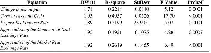
lags. That is, we found that we could not reject the null hypothesis of multivari-ate white noise for all of the orders of the Portmanteau test going fromp+ 1 to 10.In the other cases we were able to reject the null hypothesis of multivariate white noise for some orders of the Portmanteau test. Applying the criteria just mentioned, we will keep the first order VAR for the five variables case. The results for the multivariate test and some statistics concerning the estimation of every equation in the VAR are presented in Tables 2 and 3, respectively. In particular we can see that every residual does not have autocorrelation of the first order using the DW statistic17and that all of the variables in every
equa-tion are jointly significative using an F test. We also checked that the VAR(1) itself is stationary by calculating all the eigenvalues of the companion matrix of the VAR written in compact form. Since the modulus of the eigenvalues are less than one we conclude that the VAR(1) is stationary.18
As mentioned before, we will also compare the performance of the extended (full) model just estimated with one in which only the real interest rate is allowed to vary (but not the appreciation of the exchange rates) and the other in which both the real interest rate and the appreciation rates are constant. In the second case the idea is to see whether the extension of the model improves over the simpler intertemporal model and, if such is the case, the first case is used in order to determine the source of this improvement.
In order to accomplish this goal we start by estimating a VAR model that includes the change in net output, the current account and the real interest rate (but not the appreciation rate of the real exchange rates). As before, the criterion used to choose the lags to include in the VAR consists of selecting the most parsimonious VAR such that its residuals are multivariate white noise. We then estimated VARs from 5 to 1 lags, finding that the residuals can be considered multivariate white noise for every order of the Portmanteau test only for three lags (again, going formp+ 1 to 10).For the other cases we were able to reject the null for some orders of the test. We will then keep the VAR(3) as our preferred model in a system that includes the three variables. Tables 4 and 5 present the results for the Portmanteau test and some basic statistics for the estimation. We then went on to estimate a VAR with only the current account and the change in net output, which is the simplest version of the intertemporal model. We successively estimated a VAR with 5 to 1 lagsfinding, as before, that only for the VAR with three lags the residuals are white noise in multivariate sense. For the other orders of the VAR, we were able to reject the null of the multivariate white noise. Results for the multivariate Portmanteau test and some statistics for the estimated equations are presented in Tables 6 and 7. For both of the chosen models (with three and two variables) we also
17
Remember that the DW statistic is no longer valid when there are lagging values of the explained variable. In any case and as is usual in the literature, we use it as a rough indicator offirst order autocorrelation in the residuals.
18Remember that the condition for the modulus of all of the eigenvalues of the companion
matrix of the VAR in compact form te be less than one is equivalent to the condition that all of the roots lie outside the unit circle in the determinant ofΦ(L) =I−Φ1L−...−ΦPLP for
have that the modulus of the eigenvalues of the companion matrices are less than one, leading us to conclude that these VARs are stationary.
7.3
Evaluating the Performance of the Model
As was already said several times, we will test equation (8) using annual data for Argentina. In order to do so, we mustfirst have values for the parameters that appear in that equation: the discount factor (β), the intertemporal elasticity of substitution (γ), the share of tradables over total private consumption (a) and the coefficient of the appreciation of the real exchange rates (b). Of course, when testing the simpler version of the intertemporal model that includes only the change in net output (called the benchmark-model in this section), we need to deal only with thefirst of these parameters. While estimating the model that also includes the real interest rate, we have to consider also the second of the parameters. Using these parameters and the coefficients of the VAR systems already estimated in the last section for every type of model (the benchmark-model, the model with only real interest rate and the full-model) we are able to compute thek‘ vector and then theχ2 statistics to test for the validity of the
model.
Concerning the discount factor (β), from equation (2) we can see that the model implies that in the steady-state we must have thatβ= 1
1+r, where ris
the steady-state value of the real interest rate. Since in our data set the value for the sample mean of the real interest rate for the period 1885 - 2002 is negative, implying a value forβgrater that one, we will rely on the literature as a guideline to chose the value ofβ. Sheffrin and Bergin (2000) compute a value of 0.94 in their study of the intertemporal approach for Canada, Australia and the UK. Landeau (2002) computes a value of 0.95 when doing the same exercise for Chile. Vegh and Riascos (2003) and Uribe (2001) use a bit greater parameter. Thefirst authors use aβof 0.97 when calibrating their model to explain the prociclicity of public expenditures in developing countries and the second author uses a value of 0.984 when calibrating his model when studying the relation between private consumption and exchange rate behavior in stabilization plans using data for Argentina. Since the last author uses data from Argentina and for reasons that will be made clear later, we are more sympathetic towards a value of 0.98 for the discount factor.
of traded goods (a) using this decomposition, finding that the average for the period 1901 - 1997 is about 0.5 with no evident trend to raise or fall. This result is consistent with thefindings of Stockman and Tesar (1995) in their sample for developed economies.
The intertemporal elasticity of substitution is the most problematic of the parameters. Sheffrin and Bergin (2000) use values for γranging form 0.022 to 1, depending on the country. Uribe (2001) uses a value of 0.2 for Argentina in analyzing the relation between private consumption and exchange rate behavior. Landeau (2002) and Kydland and Zarazaga (2000) use a value of 0.5 for Chile in thefirst case and for Argentina in the second case.19 In what follows and in order
to reflect the probable uncertainty regarding this parameter, we will present the results concerning the estimations made with values for the intertemporal elasticity of substitution of 0.2, 0.5, 0.9 and the value that makes the predicted current account match the variance for the actual current account.
For the value ofb,wefind no reason to chose any other value than 0.5 so that we will keep this value in computing the results that follow. Of course, knowing that the test of the equation (12) is contingent on the values of the parameters just chosen, we will also consider another range for the unknown parameters to see whether there are important modifications in our conclusions.
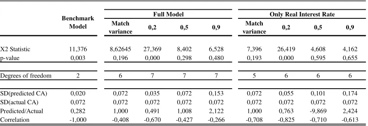
The results from the present value tests for the period 1885 - 2002 are sum-marized in Table 8. Each column of the Table represents a different specifi -cation of the model. The first column shows the benchmark - model which ignores changes in the real interest rate and the exchange rates. Columns two tofive show the model augmented with these two variables for different values of the elasticity of substitution. In particular, we first consider the value of γ that makes the predicted current account (calculated using the expression
∧
CA∗
t = k0zt) have the same variance as the actual current account and then
consider the results for the model withγ taking the values of 0.2, 0.5 and 0.9. Finally, columns six to nine are similar to columns two tofive but for the model in which the exchange rate is not permitted to vary, but the real interest rate is. This is intended to distinguish the separate effects of the two components of the consumption-based real interest rate and to try to determine, if any, the most important one. Thefirst row in each column reports the estimatedχ2 statistic
and its associatedp−value,respectively.In the third row of each column are the number of degrees of freedom used in the calculation of thep−values, which corresponds to the number of restrictions in the system (the number of elements in the vector k).20 We then present the volatility of the predicted and the
ac-tual current account (measured by the standard deviation), their ratio, and the simple correlation between the predicted and the actual current account. To illustrate further how well the restrictions of the model are satisfied, we will present somefigures with the model prediction for the current account and the
19The authors calibrate a real business cylcle model for Argentina for the period 1951
-1997.
20
actual data.21
The ratio of the standard deviations of the predicted and actual current accounts, their correlation, and their simple graph are presented as a way to in-formally evaluate the performance of the model. The actual series of the current account should equal this theoretical series whenever the model is correct. If the variance and the correlation both equal one, then both series are the same and the model is satisfied. Deviations of historical values from the theoreti-cal ones consequently provide an informal measure of the “fit” of the model. Large observed differences in the time series movements of the two variables imply (subject to sampling error) economically important deviations from the model. This evaluation may be an important complement to formal statistical tests since formal tests are often too powerful so that the merits of the model frequently became obscured by statistical rejections (Huang and Lin, 1993).
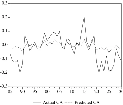
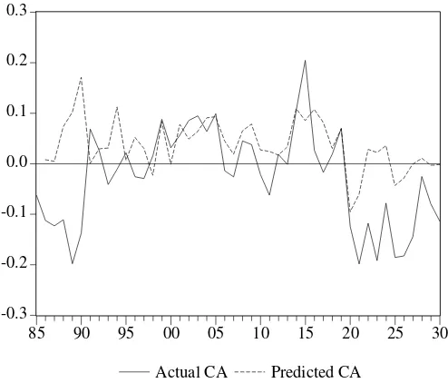
For our case, Figure 5 shows the current account variable computed from the data and the prediction generated by the version of the intertemporal model that excludes interest rates and exchange rates for the period 1885 - 2002 (the benchmark-model). This simple model is a bad predictor of the general direction of the current account fluctuations. Even worse, what is apparent from the picture is that if the Argentinean current account should have behaved as the benchmark - model predicts, one should have observed almost the opposite evolution of the current account. Even if the volatility of both series is not so different, their correlation is very negative. In total accordance with these results, the statistical test presented in column one of Table 8 soundly rejects the model. The intertemporal theory suggests that with two variables and three lags (which was the VAR selected in the last section) the k−vector accompanying theztvector should be
£
0 0 0 1 0 0 ¤while the estimatedk−vector is in fact£ 0.226 0.133 −0.016 −0.458 −0.176 −0.230 ¤.22The coefficient
on the current account at datetis -0.458853 and while it is significantly different from zero it is also different from the value of unity suggested by the theory. Further, the other values are significantly different from their theoretical values of zero. The negative values of the actual and past current account in the vector zt are at the heart of the negative relation found between the predicted and
actual current account. This result is a sharp contrast to the general tests in the area in which a simple graphical analysis suggests that the simple intertemporal model can explain much of the evolution of the actual current account without being validated by the statistical tests.
Next consider an intertemporal model which includes a time varying real interest rate and the appreciation of the exchange rates. We present in Figure 6 the predicted current account using an elasticity of intertemporal substitution of 0.9. By looking at thep−valuethis is supposed to be the less rejected of the full-models with different elasticities of substitution. From that Figure we can see that the performance of the model is as bad as that of the benchmark - model,
21Note that the
figures do not offer a way to control for the number of variables in the model. Therefore, if one is willing to make comparaisons between alternative models, we must rely primarily on the statistical tests.
22Thez
t‘ vector in this case consists of£ 4not 4not−1 4not−2 CA∗t CA∗t−1 CA∗t−2
¤
because the volatility is by far greater in the predicted current account and the correlation with the actual current account is almost zero. In column five of Table 8 we see that we can statistically reject the model. In particular, with only one lag and seven variables (remember that we included also the levels of the inverse of the commercial and market real exchange rates in the estimation of the VAR ) the theoretical k− vector should be £ 0 1 0 0 0 0 0 ¤ when it is in fact£ −0.252 −0.223 0.275 0.034 0.042 −0.335 0.458 ¤. The value for the coefficient of the current account is again negative (−0.223) and the other values seem to be significantly different from zero. Columns two, three and four show that we get similar results with other values for the elasticity of substitution. This is, we are always able to reject the model both formally and informally (thep−valuesare zero and the correlation of the predicted and actual current account is negative).23
The picture does not get better with the model that includes the change in net output and the real interest rate but not the appreciation of the real exchange rates. Even if we cannot reject the model for values ofγequals 0.5 and 0.9, the predicted current account is by far more volatile than the actual (2,418 times for aγ equal 0.5 and 3,836 times for aγequal 0.9) and the correlation is still negative.24 So, even if formally we cannot reject the model, we can do so
informally. The coefficient for the current account attin thek−vectorremains negative and the other values do not seem to be statistically equal to zero.
From what we have been saying, the intertemporal model in any of the forms (the benchmark the full model and the one with only real interest rate) do not pass the formal nor informal statistical tests for the validity of the model for the Argentine experience in the period 1885 - 2002. The model is not even capable of explaining the turning points of the Argentinean current account. So, the results just obtained show that if the Argentinean current account should have behaved as the model predicted, one should have observed almost the opposite evolution of the actual current account. We derive this result from the negative and higher correlations between the actual and predicted current accounts.
Why is the performance of the model so poor in the case of Argentina? From a statistical point of view, the problem comes from the fact that the estimated coefficients in the VAR models (in terms of signs and magnitudes) contrast with what would be predicted by the theory. For instance, we should have that the lagged values of the current account in the equation of the change in net output are negative, since from the model an increase in the current account today should anticipate a fall in the future net output. This is not what we found since we oftenfind positive signs for that variable in that equation. Changing just the signs of these coefficients makes us get by far more similar results to those suggested by the theory, than those that we get now.25
23The positive value for the elasticity of intertemporal substitution that match the variances
is 0.468.
24
Note that as with the full model, the volatility of the predicted current account rises with the intertemporal elasticity of substitution.
25Consider, for example, the model with only the real interest rate and the change in net