www.depeco.econo.unlp.edu.ar/cedlas.htm
C
C
|
E
E
|
D
D
|
L
L
|
A
A
|
S
S
Centro de Estudios
Distributivos, Laborales y Sociales
Maestría en Economía Universidad Nacional de La Plata
Simulating Income Distribution Changes in Bolivia:
a Microeconometric Approach
Leonardo Gasparini, Martín Cicowiez, Federico
Gutiérrez y Mariana Marchionni
Preliminary draft Comments welcome
The World Bank Bolivia Poverty Assessment
Simulating Income Distribution Changes in Bolivia:
a Microeconometric Approach
Leonardo Gasparini *
Martín Cicowiez Federico Gutiérrez Mariana Marchionni
Centro de Estudios Distributivos, Laborales y Sociales Universidad Nacional de La Plata, Argentina
This version: September 13, 2003
Abstract
This paper uses microeconometric simulations to characterize the distributional changes occurred in the Bolivian economy in the period 1993-2002, and to assess the potential distributional impact of various alternative economic scenarios for the next decade. Wage equations for urban and rural areas estimated by both OLS and quantile regression are the main inputs for the microsimulations. A sizeable increase in the dispersion in worker unobserved wage determinants is the main factor behind the significant increase in household income inequality in the 90s. The results of the microsimulations suggest a small poverty-reducing effect of several potential scenarios, including education upgrading, sectoral transformations, labor informality reduction, gender and race wage gap closing, and changes in the structure of the returns to education. Sustainable and vigorous productivity growth seems to be a necessary condition for Bolivia to meet the poverty Millennium Development Goal by 2015.
Keywords: distribution, Bolivia, wages, decompositions, quantile, education, MDG
JEL Classification: C15, D31, I21, J23, J31
1.
Introduction
Bolivia experienced important economic, political and social changes during the 90s following major structural reforms in the latter half of the 80s. Macroeconomic stabilization was accompanied by market reforms to increase private sector participation, align prices with market forces and increase the integration to the global economy, as well as by important political reforms to strengthen the democratic process. As part of the HIPC initiative in 2000-2001 the country developed its national Poverty Reduction Strategy with broad participation of different sectors and donors.
The Bolivian economy expanded at an average annual rate of 4.4% for most of the 90s, but decelerated to an average rate of only 1.7% during 1999-2002 in the face of external and internal shocks. The country has achieved considerable improvements in living conditions, particularly in education, health and other social indicators, although yet insufficient to meet many of the Millennium Development Goals (MDGs). Particularly, progress in reducing income poverty during the 90s was very limited and has been partially reversed with the economic stagnation that set in after 1999. Bolivia continues to be one of the poorest countries in the region. Inequality remains among the highest in the region and is a key factor as to why growth has made a small dent in poverty. The Gini coefficient for the distribution of household per capita income in 2002 was close to 60, placing Bolivia as one of the most unequal economies in Latin America, and in the world.
This paper analyzes the factors driving changes in the Bolivian income distribution by estimating wage equations from household survey microdata. We use the results of these estimations for two different microsimulations exercises. In the first one we decompose the inequality changes between 1993 and 2002 into the contribution of changes in observed characteristics of households and individuals, the returns to those characteristics and unobserved heterogeneity. We find that a sizeable increase in the dispersion in unobserved wage determinants is the main factor behind the significant increase in household income inequality in the 90s.
In the second exercise the coefficients of the wage equations estimated for 2002 are used to predict the distributional outcome of several alternative scenarios that could be generated by public policy interventions. We are especially interested in assessing the potential of each scenario in helping Bolivia reach the MDGs of halving poverty by 2015. The results of the microsimulations suggest a very modest poverty-reducing effect of a range of potential scenarios including education upgrading, sectoral transformations, labor informality reduction, gender and race wage gap closing, and changes in the structure of the returns to education. Only sustainable and vigorous productivity growth seems to be able to help Bolivia meet the poverty MDG by 2015.
considering quantile regression models. One exception arises from the fact that between 1997 and 2002 in urban areas the returns to higher education increased for the mean, but decreased for the bottom quantiles. Taking this fact into consideration by using quantile regression allows us to estimate with much more precision the impact of the changes in the returns to education on the wage and household income distributions.
The rest of the paper is organized as follows. In section 2 we present the data and show wage equations estimated by both OLS and quantile regression. The results of these estimations are used in section 3, where we characterize inequality changes in the wage distribution and the equivalized household income distribution in Bolivia between 1993 and 2002 through microeconometric decomposition techniques. In section 4 we use the estimates of the Mincer equations for 2002 to simulate the potential effect on different dimensions of the income distribution of some economic and social policy changes. Section 5 concludes with final remarks.
2.
Wage equations
In this section we first present the data, then show the results of the wage equations estimated for 2002, which serve as inputs for the microsimulations of section 4, and finally show results of the wage equations estimated for 1993, 1997 and 2002, which are the basic inputs for the decompositions of section 3.
2.1. The data
Distributional statistics come from household surveys. Bolivia has substantially improved its household surveys during the last decade. Among other things, the coverage of the survey has become national, and most sources of incomes (including non-monetary payments) have been introduced in the questionnaires. These improvements, however, introduce comparability problems among surveys in different years. For instance, the Encuesta Integrada de Hogares (EIH) of the early 90s was only urban, while the most recent Encuesta Continua de Hogares (ECH) is nationally representative. To alleviate this comparability problem we identify in the recent surveys areas covered by the early surveys to provide a “bridge” to connect results from different time periods. Table 2.1 shows the characteristics of each survey used in the paper.
We tried to make all the definitions consistent. For that reason we ignore non-monetary payments in the analysis. Also, for the decomposition of inequality changes between 1993, 1997 and 2002 (see section 3) we had to restrict the educational dummies to five categories: no education, primary, secondary, technical college and college. This specification does not allow to capture graduation or ship-skin effects, but it has the advantage of considering homogenous definitions across years. When estimating the 2002 wage equations to perform the microsimulations of section 4 we are able to expand the categories to consider incomplete and complete educational levels.
2.2. Wage equations, 2002
The estimation of wage equations is a key step for both the decomposition of past distributional changes performed in section 3 and the simulations of potential future scenarios made in section 4. We split the sample of workers into 4 groups according to two
criteria: (1) individual role in the household (household heads and non-household heads),1
and (2) type of labor market (urban and rural). Thus, we estimate the hourly earnings equations separately for household heads and non-heads, both in rural and urban areas.
The specification of the four models is almost the same. The dependent variable is the log of hourly earnings (log of wages). The vector of covariates includes the typical human capital proxies as education and age (and its squared), and other controls such as gender, ethnicity, sector of activity, geographical region, and labor-informality indicators. For the non-household heads we include an indicator of whether the individual is the spouse of the household head or any other family member.
As a measure of educational attainment we use six educational categories: no education, primary incomplete and complete, secondary complete and complete, and superior. An alternative specification could be a quadratic function of years of education. However, this is a more rigid specification, it does not allow for ship-skin effects, the variable years of education is not very reliable in the surveys of the early 90s, and moreover the gain of being able to compute returns for each year does not seem to be large, since returns are
mostly constant within educational levels.2 As explained above, we do not separate superior
education into incomplete and complete due to changes in the household surveys questions over the 90s, which make impossible to identify these two categories in a consistent way.
For the estimation of the parameters in the wage equations we use alternatively (a) ordinary least squares (OLS) and (b) quantile regression methods. The choice of OLS instead of other methods that allow controlling for sample selection is based on two considerations: (i) in absence of a good model for the selection equation, controlling for sample selection is not a dominant practice; and (ii) comparability with the estimations by quantile regressions.
1 We prefer this specification, instead of estimating models for men and women, since in the decompositions we assume that the spouse (rather than the women) takes the labor market participation decision based on the labor status of the head (rather than the men) of the household.
In what follows we provide a brief explanation of the potential advantages of estimating the wage equations also by quantile regression techniques.
Quantile regressions
Evidence for increasing within-inequality has been found in many countries, suggesting a relevant role for factors that are not captured in household surveys, like quality of
education, labor market connections, or work ethics.3 Quantile regression are designed to
take advantage of that information by modeling quantiles of the conditional distribution of
the response variable as functions of the observed covariates.4 With sizeable unobserved
heterogeneity mean linear regression models provide only a limited characterization of the dependent variable as a function of covariates, since this is modeled as a unique function of the covariates. In particular, models seek to find the relationship between the observed covariates and the mean of the conditional distribution of the response variable. This characterization leaves useful distributional information outside the model. The technique of quantile regression, introduced by Koenker and Basset (1978), can provide a richer characterization of the conditional distribution of the dependent variable when the
regression errors are not iid. Although quantile regression was originally proposed as a
robust alternative to OLS for estimating the parameters of a linear model, the literature has used this technique for revealing how the covariates affect the entire shape of the conditional distribution. To provide a brief idea of quantile regression, write a wage equation as
(2.1) w = Xβ + ε
where w is the (log) hourly wage, X is a vector of covariates, β a vector of parameters, and
ε a vector of independent error terms. The θ-th conditional quantile of w can be written as
(2.2) Qθ(w\ X)=Xβ(θ)
where the θ-th conditional quantile of the error term is assumed to be zero. Equation (2.2)
can be defined for a set of quantiles θ, given rise to a family of quantile regression curves,
which provide a more detailed characterization of the relationship between X and w.
Naturally, the most interesting case is when the estimated β(θ) coefficients differ across
quantiles θ, suggesting that the marginal effect of a particular explanatory variable differs
across quantiles of the conditional distribution of w.
Suppose X is just years of formal education. OLS provides a single β, and hence a single
estimate of the returns to education for the whole population. Returns to education however may depend on some unobservable factors, like education quality, talent, or labor market connections, and hence they may differ across groups of these factors. Quantile regressions
3 See Buchinsky (1994) and Juhn et al. (1993) among others.
provide a parametric way to assess these potential differences. By modeling the conditional distribution of wages by quantile regression, we allow the unobserved component of wages to interact with the available measures of observed skills. Moreover, it allows to recover features of the entire distribution without imposing any a priori shape such as normality.
Results
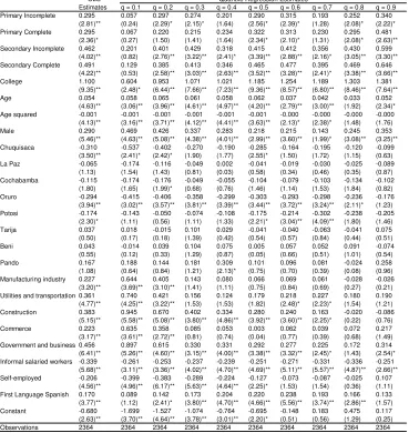
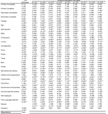
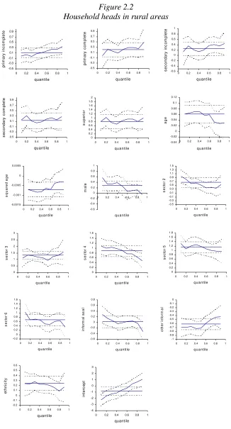
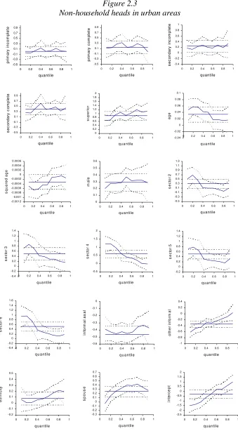
In what follows we present the results of the wage equations for 2002 estimated by OLS and quantile regression techniques. The results described here correspond to the specification used for the simulations in section 4. Tables 2.2 to 2.5 report OLS and quantile regression estimates for each of the four sample groups considered. These results are also plotted in Figures 2.1 to 2.4, where we show the estimated quantile regression coefficients, the mean effect estimated by OLS, and the corresponding 95% confidence intervals.
Estimations by OLS produce positive returns for each educational level and, at least for the higher levels (beyond secondary education), they are always significant. For household heads in urban areas each level significantly contribute to increase hourly earnings. Primary school increases the mean wage of this population group in almost 30%. However, there seems to be no difference in wages from having some primary education and finishing that educational level. The returns for secondary incomplete, secondary complete and superior are 46%, 49% and 110% respectively, compared to a similar household head worker with no education. It is interesting to notice that for urban non-heads workers and for rural workers having incomplete primary education does not add to wages, while the contribution of having a primary education degree is small and probably non-significant.
Unexpectedly, the quantile regression estimates are quite consistent with the ordinary least square estimates. It is clear from the figures that the quantile regression estimates lie inside the 95% confidence interval for the estimated mean effect in most cases. One of the exceptions to this pure location shift effect for the group of urban household heads appears at the lowest quantile (0.10), where in contrast to OLS estimates, high school completion and college education have almost no returns in terms of wages. There are also some cases in which for the higher quantiles the estimated return significantly exceeds the mean effect.
The specification adopted for the hourly earnings equations includes age and its squared to
capture non linearities in the returns to aging, potentially related to work experience. Except for the group of non-household heads in rural areas, age has a significant concave (mean) effect on wages. For household heads, both in urban and rural areas, aging increases wages up to age 45 approximately. Again, the quantile regression estimates do not differ significantly from the estimated mean effect. Despite this fact, at the lower quantiles the wage-age profiles appear to be more concave. For household heads in urban areas, for example, hourly earnings for the first quantile increase between ages 14 to 40 and then decreases, while for the highest quantile wages continue increasing up to age 52, amplifying the wage gap.
woman with similar characteristics. For the rest of the groups the wage gap in favor of men hovers around 28%. This effect appears to be slightly decreasing by quantiles for household heads, possibly reflecting the higher dispersion of female earnings. For household heads in rural areas, for example, for quantiles 0.6 and higher the gender effect is not significant. For non-household heads the gender effect seems to be quite constant across the conditional distribution of the independent variable.
To control for the potential effect of the worker sector of activity on wages we include five sectoral dummies: manufacturing industry, utilities and transportation, construction, commerce, and skilled-labor intensive services (government, education and business). The omitted category is the primary sector (agriculture, fishing and mining). In general, the mean effect of not being in the primary sector is to increase hourly wages. This effect is particularly high for household heads in rural areas, where the return to working in the manufacturing industry or in the skilled-labor intensive services -compared to the primary sector- is approximately 65%, while working in commerce has the (mean) effect of more than duplicating wages. In contrast to other variables, the effect of sector of activity on wages varies significantly across conditional quantiles, especially in urban areas. Generally, not being in the primary sector has a stronger effect for the lower quantiles and sometimes insignificant for the higher ones. This might be caused by a relatively higher dispersion of earnings in the primary sector.
According to OLS estimates the effect of informality in urban areas is to reduce wages, both for informal salaried workers and the self-employed. In rural areas informality appears to have a negative effect, though not always significant, only for salaried workers. Regarding the quantile regression estimates, the effect of informality for wage-earners is generally consistent with the results from OLS estimation. In contrast, for the self-employed informality has strong negative effects for the lower quantiles, and - depending on the case- no effect or even positive effects for the upper quantiles. This fact is consistent with high heterogeneity within this group, which comprises self-employed workers of very low productivity and highly productive self-employed professionals.
For the 2002 survey we have information on the first language spoken by the worker, which we use as a proxy for ethnicity. The indicator takes the value 1 for individuals who have Spanish as their first language. According to OLS estimates, having Spanish as the first language has a positive effect on wages for household heads, while it is unimportant to determine wages of other population groups. For household heads in urban areas the mean effect is a 17% increase in wages, while for rural areas it hovers around 25%. Estimates by quantile regression do not differ significantly from the estimated mean effect.
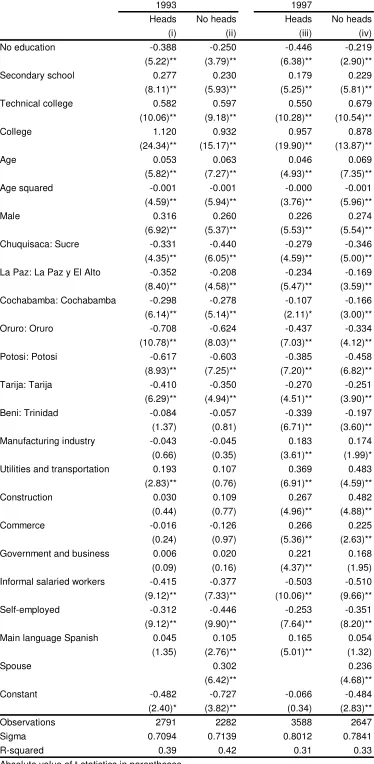
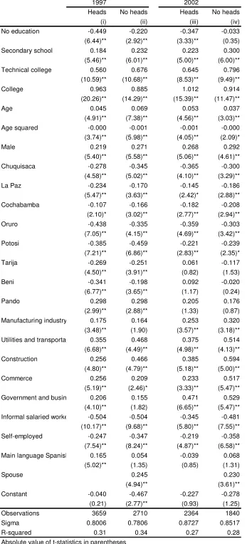
2.3. Wage equations, 1993-2002
Tables 2.6 and 2.7 show the results of estimating the wage equations by OLS. To help interpret the results regarding the returns to education, Figures 2.5 to 2.7 depict the predicted hourly wages as a function of the educational level for male household heads aged 40 living in Santa Cruz de la Sierra, working in the manufacturing industry in a formal job. In each figure values are normalized so that wages for those with primary education coincide in both years. Returns to education are always positive. The wage-education profile became less convex between 1993 and 1997 in the main cities of Bolivia, as the returns to college education significantly decreased, implying an equalizing effect on the wage distribution.
In contrast, returns to a college education increased between 1997 and 2002 in urban areas. This change in the wage-education profile implies an inequality-increasing effect on the hourly earnings distribution, and also on the equivalized household income distribution, since workers with a college education are located in the upper tail of that distribution. From the figures, this unequalizing effect, however, seems to be weaker than the equalizing effect of the early 90s. Similar changes have occurred for spouses and other members of the household.
Figure 2.7 does not show a clear pattern of change in the returns to education in rural areas between 1997 and 2002. Returns to primary education and secondary education fell relative to no education, while there was a large increase in the returns to those with a non-university superior education. The aggregate effect of these changes on wage inequality is not clear. The decomposition can help us to assess the sign and size of these effects on the income distribution.
The standard deviation for the distribution of the regressions residuals are shown under the
label of sigma in Tables 2.6 to 2.7. These residuals are usually interpreted as capturing the
effect of unobservable factors like natural school quality, ability, labor market connections,
or work ethics on wages. The values of sigma in the table suggest that the dispersion in
these unobservable factors have substantially increased in Bolivia over the last decade both for heads and non-heads. This fact could be the consequence of an increasing dispersion in the endowment of the unobservable factors and/or an increase in the “returns” to these
endowments. The latter interpretation has been the dominant in the literature (see Juhn et
al., 1993), and it is particularly more compelling for short periods of time. The increase in
the values of sigma is sufficiently large to believe that a sizeable proportion of the overall
increase in the dispersion of wages can be due to this factor. The decomposition analysis will assess this relevance within a more rigorous framework.
As in most countries, in Bolivia men earn more than women even when controlling for observable characteristics. According to the results of the wage regressions the gender wage gap has significantly shrunk between 1993 and 1997, but has widened again in the next 6 years, both in urban and rural areas.
they increased for quantiles 0.5 and 0.9. For technical college the increase in the returns is very small for quantile 0.1 and much larger for the rest, while the returns to secondary school fell for quantiles 0.1 and substantially increase for quantile 0.9. Similar divergent patterns for the change in the returns to education across conditional quantiles are present in the results of Tables 2.8 and 2.10.
3.
A characterization of inequality changes, 1993-2002
In this section we show inequality patterns for Bolivia during the last decade, present a methodology that helps to characterize distributional changes, and report the results.
3.1. Income inequality in Bolivia
Bolivia is, and has been for decades, one of the most unequal countries in Latin America, and in the world. This fact combined with low per capita GDP account for the high poverty levels of the country. Figure 3.1 shows the Gini coefficient for the distribution of household equivalized income for several countries in Latin America and the Caribbean (LAC) around year 2000. Bolivia clearly stands as a high-inequality country.
The focus of this section is not on the relative position of Bolivia in the region, but instead on the factors underlying the persistent highly unequal income distribution in the last decade. In particular, we divide the decade into two periods according to the growth performance: 1993-1997, a period where the economy grew at an average rate of 4.5%, and 1997-2002, a period of stagnation.
Column (i) in Table 3.1 shows the Gini coefficient for the distribution of household equivalized income, defined as total household income divided by the number of adult equivalents raised to a parameter that captures household economies of scale (see Deaton
and Zaidi, 2002).5 Household income comprises labor and non-labor income and includes
only monetary payments, since non-monetary payments are not available in all surveys in the period under analysis. The Gini coefficient for the distribution among individuals of equivalized household income remained constant around 50.3 between 1993 and 1997 in the urban areas covered until mid 90s. In the next 6 years the Gini for these areas increased 3 points, while inequality for the whole country increased 2 Gini points, which represents a
substantial increase.6 Confidence intervals computed by bootstrapping techniques, shown
below the Gini coefficients in the table, confirm the significant inequality increase between 1997 and 2002.
5 The denominator is
(
α α)
θ2 2 1
1.K .K
A+ + , where A is the number of adults, K1 the number of children under 5 years old, and K2the number of children between 6 and 14. Parameters α allow for different weights for adults and kids, while θ regulates the degree of household economies of scale. Following Deaton and Zaidi (2002) for less-developed economies like Bolivia we take intermediate values of the αs (α1=0.5 and
α2=0.75), and a rather high value of θ (0.9) as the benchmark case.
Labor is the most important income source captured by the household surveys in Bolivia (around 90% of total income). Given the difficulties in modeling capital income and transfers, in most of the rest of the paper we ignore these income sources and work with household income obtained only from labor sources. Column (ii) in Table 3.1 shows the
Gini for the distribution of equivalized household labor income in the survey. In column
(iii) we restrict the analysis to households included in the microsimulation. They are basically households with complete and consistent answers not living exclusively on rents and pensions. The trends in inequality for the more restricted variables in columns (ii) and (iii) do not significantly varied from the trend of the more general variable in column (i).
The second panel in Table 3.1 shows that inequality in wages and earnings has also significantly increased in Bolivia in the last decade. That pattern is clear when working
with both all the survey and the subsample used for the decompositions.7
3.2.Decomposing distributional changes with OLS wage equations
Decompositions provide counterfactual distributions that are helpful to characterize past changes in inequality and poverty, and to make predictions on the distributional impact of future changes in economic factors and public policies. Microeconometric decomposition
techniques (also known as microsimulations) have been initially applied to the study of
discrimination (Blinder, 1973; Oaxaca, 1973; Oaxaca and Ramson, 1994), and more
recently in the inequality literature (Juhn et al., 1993; Bourguignon et al., 2001). In the last
few years, this methodology has become a usual tool for the analysis of distributional changes (Bourguignon, Ferreira and Lustig (eds.), 2003). We first provide a brief
explanation of this methodology and then show the results for Bolivia.8
The basic idea of the decompositions is to simulate the distribution in time t1 if some of its
determinants (parameters or distribution of covariates) were those of time t2, and compare
that counterfactual distribution to the real one in t1. The difference between the two
distributions can be attributed to the change in the selected determinants between t1 and t2.
Let Yit be individual’s i labor income at time t, which is written as a function F of the
vector Xit of individual observable characteristics affecting wages and employment, the
vector εitof unobservable characteristics, the vector βtof parameters that determine market
hourly wages and the vector λt of parameters that affect employment outcomes
(participation and hours of work).
(3.1) Yit =F(Xit,εit,βt,λt) i=1,...,N
where N is total population. The distribution of individual labor income can be represented
as
7 The use of other inequality indexes does not change the picture of inequality trends. Results for other indices are available from the authors upon request.
(3.2) Dt =
{
Y1t,...,YNt}
We can simulate individual labor incomes by changing one or some arguments in equation
(3.1). For instance, the following expression represents labor income that individual’s i
would have earned in time t if the parameters determining wages had been those of time t’,
keeping all other things constant.
(3.3) Yit(βt')=F X( it,ε β λit, t', t) i=1,...,N
More generally, we can define Yit(kt’) where k is any set of arguments in (1). Hence, the
simulated distribution will be
(3.4) D kt( t')=
{
Y1t(kt'),...,YNt(kt')}
The contribution to the overall change in the distribution of a change in k between t and t‘,
holding all else constant, can be obtained by comparing (3.2) and (3.4). The comparison between the actual and the counterfactual distributions can be made in terms of any indicator of any dimension of the distribution (e.g. poverty, inequality, polarization, aggregate welfare). For instance, if we are interested in inequality comparisons, and we
define an inequality index as I(D), the effect of a change in argument k on earnings
inequality will be given by
(3.5) I(Dt(kt'))−I(Dt)
If, for instance k = βed (i.e. the parameter linking education with hourly wages), equation
(3.5) will provide an estimate of the effect of changes between time t and t’ in the returns to
education on earnings inequality.
In order to compute (3.5) we need estimates of parameters β and λ and the residual terms ε.
We adopt an econometric specification similar to the one used by Bourguignon et al.
(2001), which corresponds to the reduced form of the labor decisions model originally
proposed by Heckman (1974).9 The model has two equations, one for wages and one for
the number of hours of work, where the error terms represent unobserved factors affecting the determination of endogenous variables.
Results
Table 3.2 shows the main results of applying this methodology to the case of Bolivia for the distributions of hourly wages and equivalized household labor income. The results shown are averages over the simulations using alternatively the first and second year as base years. As it was explained the microsimulations generate counterfactual distributions. For simplicity we just report the Gini coefficients of these distributions, but other inequality indices and measures of other dimensions of the distributions are available upon request.
To explain the table, let’s concentrate in panel B, which shows the results for the decomposition of changes between 1997 and 2002 in urban areas. The Gini coefficient for
the hourly wage distribution increased 2 points between those years.10 If only the returns to
education had changed in that period the Gini would have gone up just 0.2 points, according to the estimates of model 1. This means that the returns-to-education effect has been unequalizing, confirming the presumption from the previous section.
Model 1 corresponds to the specification shown in Tables 2.7 and 2.8. We have worked with a large number of alternative specifications. In the table we show two alternative models where sectoral and informality dummies are ignored. Also, in model 2 wage equations are estimated separately for spouses and other members (instead of just non-heads). Although the main qualitative results are quite strong to different specifications, the magnitudes of some of the effects are unstable. For instance, the returns-to-education effect that seems small in panel B when using model 1, becomes more important when using model 2.
As discussed before changes in the returns to education were inequality-decreasing between 1993 and 1997. According to the results of the decompositions, the direct impact of these changes was a fall in wage inequality of around 1 Gini point. That change translated into a drop in equivalized household income inequality of the same size. In contrast, changes in the returns to education in urban areas between 1997 and 2002 were unequalizing, although smaller compared to the changes in the early 90s. In rural areas the inequality impact of the change in the wage-education profile turns out to be negligible.
The gap between skilled and unskilled workers has widened in terms of hours of work over the last decade: while college graduates worked in 2002 around 3 hours more per week than in 1997, those with only primary-complete worked on average 2 hour less. These changes have had an unequalizing effect on the distribution, which shows up in Table 3.2. However, the impact seems to be modest: in none of the cases the Gini increases more than half a point due to this factor.
According to the results shown in section 2 the gender wage gap shrunk between 1993 and 1997, and increase thereafter. This pattern shows up in the results of the decompositions as an equalizing change on the wage distribution in panel A, and an unequalizing change in panel B. However (i) the size of these effects is small, and (ii) the impact on the household income distribution becomes non-significant. This latter result is likely the consequence of working women being disproportionally located in the upper part of the household income distribution.
The most relevant change among those considered in the Table is the increase in the dispersion of unobservables. That effect alone accounts for an increase of more than 3 Gini points in the distribution of wages between 1993 and 1997, 3 points between 1997 and
2002 in urban areas, and 2 points in rural areas. The impact on the equivalized household income distribution is smaller, although still quite relevant.
The regression for rural areas in Table 2.7 suggests significant regional changes between 1997 and 2002, which basically implies a reduction in the wage gap between several regions and Santa Cruz. These changes are reflected in a relatively large equalizing effect on the income distribution in rural areas, since Santa Cruz is a relatively rich region.
Changes in the educational structure of the population can modify the distribution of wages and earnings, and in turn the distribution of household income, through several channels. Suppose that during a given period of time a group of individuals change their educational status from primary complete to college complete, and correspondingly the distribution of
expected wages change for them.The increase in wages for those individuals will certainly
tend to reduce poverty. The effect of this education upgrading on inequality is ambiguous. To illustrate the point with an extreme example, suppose that previous to the shift all the population were in the primary complete group. The shift will then be clearly unequalizing. In the other extreme if people who become more educated were the only left in the primary education group and the rest of the population were in the college group the change will be
equalizing.11 A second channel could be important: given that the within dispersion of
wages usually differ across educational groups, the change in the educational structure will affect overall within-inequality. Finally, there is an indirect effect of education on wages, which could be very important in the medium or long run: an increase in the supply of skilled workers contribute to a fall in the wage premium for that group, lowering the dispersion in wages and earnings.
In Table 3.3 the adult population is classified into five educational groups. The proportion of adults with less than primary education is very high, although has decreased over time. The share of those with a secondary and college education (non technical) has increased over the analyzed period. The reduction of the non-education group and the increase in the college group probably imply an unequalizing effect. However, since there are other changes in the distribution of education, the final distributional effect is not clear. The microsimulations allow us to better assess this point. The results of Table 3.2 suggest that the effect of changes in the educational structure was unequalizing. The size of that effect is modest between 1993 and 1997, large in urban areas between 1997 and 2002, and small in rural areas. The educational upgrading in urban areas in Bolivia in the late 90s can account for 1 extra Gini point of wage inequality and 1.5 Gini points of household income inequality.
It is interesting to notice that the sum of all effects considered in the paper account for an increase in inequality greater than the actual change, which means that factors not considered in the analysis may have played a relevant equalizing role.
Summing up, changes in the returns to education were an equalizing factor in the early 90s and an unequalizing although minor factor thereafter. Changes in the gender wage gap did not significantly affect household inequality. In contrast, the increase in the returns to
unobserved worker characteristics has played a very significant unequalizing role over the last 10 years. Changes in regional wage gaps have played an equalizing role, especially in rural areas. Finally changes in the education structure have been mildly unequalizing.
Given the results of this section regarding the relevance of the returns to formal education and the endowment of unobservable factors in accounting for the changes in income inequality, the next section will deepen into the analysis of these factors by using quantile regression analysis.
3.3. Decomposing distributional changes with quantile regression
The quantile regression estimates are used to enrich the decomposition analysis.12 Instead
of estimating a single β and simulating the distributional impact of its change, by using
quantile regressions we can estimate a family of β(θ) and find the counterfactual
distribution when the whole family of βs change. Also, we can make the decomposition
analysis separately for changes in each of the β(θ). This procedure may provide a richer
characterization of past changes in the income distribution, as well as a richer characterization of future distributional changes generated by economic and social changes or policy interventions. Additionally when simulating changes in the educational structure, we can simulate the new individual wage from upgrading education according to the wage-education profile of the particular quantile to which the individual “belongs”.
Let βˆt(θ) be the estimated parameters of the wage equation in time t. Individual i’s wage
can be expressed as
(3.6) wit = Xit'βˆt(θj)+µit(θj)
where j=1,...,J indexes the quantiles. Notice that wit can be expressed in relation to any of
the J quantiles with a different error µit for each alternative expression.
Now define
(3.7) * arg
{
( )}
j it
it min j µ θ
θ = θ
θ*
it defines the quantile for which the regression line is closest to the individual actual
observation. We can write
(3.8) wit = Xit'βˆt(θit*)+µit(θit*)
We propose the following counterfactual wage of i in t1 if parameters βs were those of time
t2
(3.9) ( ) ˆ ( ) 1( *1)
* 1 2 ' 2
1 it i i i
i X
w β = β θ +µ θ
We are assuming that in time t1 individual i “belongs” to the θ*i1th quantile of the
conditional distribution of w, and then we apply the time t2parameters βs corresponding to
that quantile. We then add the error in t1 as we want to keep this term fixed.
The interpretation is the following. Suppose the wage w is a function of formal education X,
which is observable by the analyst, and by innate talent and pure chance, which are unobservable. The effect of formal education on wages depends on ability but not on
chance. Suppose we believe there are J groups of ability and estimate J quantile
regressions. We assume that i belongs to the θth group of ability if its actual wage is
“similar” to the predicted one for the θth regression given i’s observable education Xi. The
difference between the actual wage and the prediction is attributed to the effect of pure chance.
Suppose that for some reason the way education and talent affect wages changes between
time t1 and t2, which causes the family of parameters βs to change. To simulate individual
i’s new wage we assume that she will remain in the same θthgroup of ability, and that she
will be equally lucky than before. In particular the effect of luck on the wage will be the same as before. This is the intuition behind equation (3.9).
Of course the partition of unobservables between talent, which is modeled through quantiles, and luck, which is left as the residual is completely arbitrary. In the limit we can
estimate enough quantile regression so that the residual µ disappears. However, we find this
alternative (i) computationally more cumbersome, and (ii) intuitively less compelling.
Given the exploratory character of the decompositions by quantile regression we limit the empirical analysis to just the returns to education using the model specification 1. Table 3.4 shows the results in terms of the Gini coefficient. Compared to the results obtained by OLS, the effect on income inequality of the changes in the returns to education appears to be magnified by using quantile estimations. While the fall in the returns to education between 1993 and 1997 accounts for a drop of 1 Gini point using OLS, the fall is 2.5 Gini points by using quantile regression. During 1997 and 2002 the returns to education increased, a fact that contributed to increase wage and household income inequality. While with OLS estimations the impact on inequality was just 0.2 Gini points, the effect grows to 1 point with quantile estimates. Finally, in rural areas the distributional impact of the changes in the returns to education between 1997 and 2002 is estimated as negligible by OLS, and significantly unequalizing by quantile regression.
the conditional wage distribution, who are likely also located in the upper quantiles of the unconditional wage distribution. Therefore, the unequalizing effect of this change is likely to be greater.
4.
Simulating economic and policy changes
In this section we carry out some simple simulations to provide estimates of the distributional impact of different growth scenarios. In particular we are interested in assessing the potential impact of different policy changes in helping to achieve the Millennium Development Goal (MDG) of reducing poverty by half between 1990 and 2015.
The starting point is the observed income distribution in 2002. We postulate several impulses and trace their impact onto three dimensions of the income distribution: the mean (growth), the income dispersion (inequality), and the mass below a certain cut-off income point (poverty). It should be stressed that these are rather statistical exercises, where after a proposed impulse, all parameters and individual characteristics are kept constant.
4.1. Growth and inequality: some mechanical exercises
We start with some mechanical exercises in which we consider alternative growth rates in per capita income and assume an invariant distribution (except for the increase in the mean). Table 4.1 shows statistics for the resulting income distributions in 2015 of
simulating five different annual growth rates (g): 1%, 3%, 5%, 6.5% and 8%. For each case
we report the mean income of the distribution, along with ten widespread inequality indicators, and three poverty measures, both for moderate and extreme poverty, and also
separately for urban and rural areas.13
The results of Table 4.1 on mean income and inequality are trivial, given the nature of the exercise. More interesting are the results on poverty. According to these exercises growing at an annual rate of 1% for the next 13 years with no changes in the income distribution would reduce poverty and extreme poverty in Bolivia, as measured by the headcount ratio, in around 5 points, which would certainly fall short of the MDG. The impact would be even more modest in rural areas with a fall of around 3 percentage points. Obviously, a higher annual growth rate has a greater impact on poverty. The national headcount ratio could be reduced to 50% with an annual growth rate of 3% and to 40% if the Bolivian economy could grow at 5% until year 2015.
The MDGs propose halving poverty between 1990 and 2015. Unfortunately, Bolivia does not have reliable statistics on poverty for the early 90s, since the household surveys were not nationally representative by that time. By extrapolating changes in poverty for the main urban areas between 1992 to 1997, and for the whole country between 1997 and 2002, we estimate that the headcount ratio in the early 90s would have been just 3 points higher than
in 2002. As Table 4.1 shows, we estimate income poverty for 2002 in 65.1%.14 That implies that the MDG for Bolivia would be a national poverty headcount ratio of around 34% by 2015. With an invariant income distribution that goal could be met if the economy grew at an annual rate of 6.5% for the next 13 years, which seems to be an ambitious scenario. The national headcount ratio would be decreased to 29% with an annual growth rate of 8%. However, notice that even in this case poverty in rural areas remains very high (54%), not reaching the MDGs of halving the headcount ratio.
Table 4.2 shows the poverty-growth elasticities for each scenario. Each entry in the table represents the change in the headcount ratio (in percentage points) for each 1% growth in mean income. The “productivity” of growth in terms of poverty reduction is decreasing in the growth rate. The poverty impact of this distributional neutral economic growth is higher in urban than in rural areas, except when considering extreme poverty in scenarios of high economic growth. Figure 4.1 helps to understand this result by showing kernel estimates of the density functions for the distribution of household per capita income in urban and rural areas. The vertical lines represent the “average” poverty lines for each area. Notice that the mass around the poverty line in urban areas is larger than in rural areas. An increase in real income can be represented as a movement of the poverty line to the left with an invariant nominal income distribution. Notice from Figure 4.1 that a small shift of the poverty line to the left affects more people in urban areas than in rural areas.
In Table 4.3 we model simple redistributive policies with no efficiency losses. In particular
we assume a proportional income tax of rate t with an egalitarian distribution of the
revenues.15 Three tax rates are considered in the Table: t=.1, t=.2 and t=.3. These changes
have no impact on mean income and a rather trivial effect on inequality. The impact on poverty are more interesting to analyze. Even with a high tax rate of 30% the headcount
ratio would be far from the MDG (58%).16 This result highlights an important point: given
that Bolivia is not only a country with high poverty indicators, but also a poor country in terms of mean income, there are no large gains in terms of poverty from pure redistributive policies, at least of the form proposed in this exercise. Of course, it should be stressed again that these are just statistical exercises. It can be argued that even small redistributions are
enough to help the poor to build capacities (e.g. education) and escape poverty. However,
this kind of (certainly very relevant) exercises are out of the scope of this paper.
Notice also that extreme poverty is more sensible than moderate poverty to the reditributive
policies of the kind considered here, i.e that imply a lump-sum payment to people with
income lower than the mean. A not-too-high income transfer is enough to drive many households out of extreme poverty. The goal of halving extreme poverty could be reached
with t=0.2.17
14 This figure is a little higher than the official figure since we use income and not expenditures for rural areas. We follow this procedure in order to be able to apply the models developed in previous sections to estimate and predict earnings.
15 Paes de Barro et al. (2002) have recently carried out similar exercises for LAC.
16 Only with a rate of t=.55 Bolivia would meet the MDG. However, it is hard to imagine such massive redistribution policy not having negative effects on accumulation and hence mean income.
We also simulate the direct impact on the household per capita income distribution of an increase in the productivity of labor. As Table 4.4 shows an annual 1% rate of growth in earnings for all workers until 2015 would imply a fall of just 4 percentage points in the national poverty headcount ratio. An annual productivity growth of 5% implies a much greater impact: poverty will be reduced from 65.1% to 44.9% and extreme poverty from 41.8% to 26.7% by 2015. In the two last columns we repeat these exercises but changing only earnings for those individuals for which we estimated wage regressions in section 2. Since in the following section we change variables only for these individuals and trace the distributional impact, it is important to assess how much we lose by ignoring income changes for the rest of the population. The results of Table 4.4 suggest that the loss would be rather small.
In Table 4.5 we simulate a 5% annual growth in earnings for workers in each sector separately. The differential impact of the earnings increase depend on the number of poor people (and their incomes relative to the poverty line) working in each sector. From Table 4.5 the impacts do not seem to differ substantially across sectors, except for the expected larger impact of an increase in the productivity of primary activities in rural areas.
Figure 4.2 shows the resulting growth-incidence curves after a annual 5% increase in earnings in all sectors, in primary activities and in skilled-intensive service sectors. A growth-incidence curve shows the growth in household per capita income for each quantile of that distribution after a given perturbation. Generalized earnings growth is about neutral, pro-poor if it takes place in the primary sector, and pro-rich if it happens in the skilled-intensive sectors.
Table 4.6 shows the average individual growth rates in per capita household income computed for three groups: those below the extreme poverty line, those between the poverty line and the extreme poverty line and the non-poor. The average of the growth rates for the poor is proposed by Ravallion and Chen (2003) as a measure of pro-poor growth. A 5% increase in the productivity of labor in the primary sector implies a pro-poor growth rate of 2.6% (considering the extreme poverty line). It is interesting to compare the first two rows in Table 4.6 with the third one. An increase in productivity in the primary sector will imply higher household per capita income growth for the poor than for the rest of the population. This is not the case for the rest of the sectors, especially for the skilled-intensive sectors (government and business).
We also simulate a labor productivity increase in urban and rural areas separately to assess the potential impact on poverty of regional targeted policies. A 5% annual growth in earnings in urban areas reduces poverty in that area from 53% to 29.1%. A similar productivity increase in rural areas would reduce poverty from 85% to 70.9%. Table 4.7 shows that the pro-poor growth rate of an earnings increase is higher in the rural areas. The growth-incidence curves in Figure 4.3 are illustrative of a higher impact on poverty for policies targeted in rural areas.
characteristics and the returns to those characteristics. For simplicity we compute the impact of each change in characteristics or returns only on the hourly earnings of each working person, and with this simulated wage we reconstruct household per capita income. To simulate wages we use the models in section 2 estimated both by OLS and quantile regression.
4.2. Changes in individual characteristics
In this section we change some selected individual characteristics - education, sector of activity, type of work and number of children - and assess their impact on the income distribution. For illustration purposes, take the case of education. We follow a 5-step procedure.
1. Propose a change in the education structure of the population. Potential scenarios are
generated by extrapolating actual trends and/or by considering policy goals.
2. Change individual education to replicate the target structure of step 1. Changes are
made in a “natural” order. If we propose a new scenario with a larger college group, we draw the new college-educated workers from the former secondary-complete workers.
3. Predict wages for those individuals whose education was changed in step 2. For this
step we classify workers into household heads and non-heads, and living in urban or rural areas and use the relevant regression to predict wages. We alternatively use OLS and quantile regression models, and predict wages following the procedure described in section 3. We restrict the analysis to those individuals in the sample used to run the Mincer regressions of section 2.
4. Reconstruct earnings and household per capita income with the new information.
5. Compute statistics for the new simulated household per capita income distribution.
Education
Table 4.8 shows the 2002 distribution of workers into the 6 educational categories considered. The first scenario (s1) is the consequence of extrapolating trends in the 90s to
2015.18 The second scenario (s2) is generated by assuming an acceleration of the 90s
trends. The last two scenarios are ambitious policy objectives of eliminating illiteracy, substantially increasing primary school completion, and increasing high school and college attendance.
The distributional results of microsimulating these changes are shown in Table 4.9. The income distribution does not seem to substantially vary after the simulated changes in the educational structure of the working population. Mean income grows less than 1 percentage point in scenarios 1 and 2, and a rather modest 5% and 6% in the two last more ambitious educational scenarios. Income inequality decreases very slowly as we alter the educational structure. As a consequence of these changes in mean income and inequality the simulated decrease in poverty turns out to be very modest. The national poverty headcount ratio would fall just ½ point if the educational trends of the 90s continue in the next decade. A
more ambitious educational upgrading would not generate spectacular distributional outcomes either. For instance, poverty would fall just 3 points in the scenario s4, clearly falling short of the MDG. Impacts are just a little bit greater for rural extreme poverty but still disappointing. Qualitative results are similar using different poverty indicators. Also OLS and quantile regression yield similar results, as it was expected from the analysis of section 2.
Table 4.10 may help clarifying the perhaps surprising result of a minor distributional impact of the educational upgrading. The Table shows the working population aged 30 to 50 in urban areas classified by education. Column (iii) reproduces the resulting educational structure under scenario s4. Even after a sizeable change in the educational structure the average wage just grows 8%, which suggest a minor impact on poverty. The impact would be in fact even more modest due to at least two factors.
First, recall that extreme poverty in urban areas is around 26%. Assume that household income is perfectly correlated with worker’s education and hence, from Table 4.10, that those with no education and with primary incomplete are the ones below the extreme poverty line in 2002. An educational upgrading that moves some workers with primary incomplete to primary complete would not have a big impact on poverty, since the wage premium of finishing primary schools seems to be small as discussed in section 2.
Second, the correlation between education and other wage determinants may further reduce the potential impact of an educational upgrading. Suppose all primary-incomplete workers were women, where in the primary–complete half were men and half women. An educational upgrading would drive women to the primary-complete group. If as data suggests women earn less than men, the new primary-complete workers would earn less than the average of that group previous to the educational upgrading. This fact implies a lower impact on poverty than Table 4.10 suggests. The example is obviously unrealistic. However, it is true that education and gender are highly correlated: 49% of workers in Table 4.10 with primary incomplete are women, while nearly 70% of those with primary complete are men. Also, men with primary complete earn 20% more than women with the same educational degree.
A third potential source of a reduced impact of educational upgrading on poverty would arise if the returns to education were flatter for the lower conditional quantiles. In that case the impact of an educational upgrading would be lower for workers with low values of unobserved characteristics, who are also those more likely to be close or below the poverty
line.19 This effect, however, does not seem to be present from the results of Table 4.10, as a
consequence of the results obtained by OLS being similar to those obtained by quantile regression.
Tables 4.11 to 4.13 investigate the relationship between poverty and growth after the impulse of an educational upgrading. A change in the educational structure modifies incomes for some people, which in turn is reflected in mean income growth and poverty changes. Growth and poverty are then “dependent variables” in this exercise. Hence, poverty-growth elasticities should be seen as just correlations of the change in income and poverty as the economy is perturbed by an impulse. In Table 4.11 we report these elasticities for the 4 simulations of changes in the educational structure.
The growth-incidence curves of Figure 4.4 suggest a minor and uniform impact of scenario s1, and a larger and inverse-U shaped impact of scenario s4. Mean growth rates for different income groups are presented in Table 4.12. In this case we report the total growth (and not the annual growth rate) from comparing the distribution before and after the change in the educational structure. The pro-poor growth rate is just above 1% in scenario s1, and a still modest 8% in scenario s4.
In Table 4.13 we perform a Datt-Ravallion decomposition of the change in poverty by microsimulating the income distribution if only the mean changed after a given shock. In the simulation s4 the national poverty rate falls around 3 points: 2 of them are the “result” of changes in the mean of the distribution, while 1 extra point comes from a more equal distribution generated by the new educational scenario.
Sector of activity
We simulate 4 scenarios regarding the sectoral structure of employment (see Table 4.14). The first one (s1) extrapolates changes occurred in the 90s into the next decade. The second one (s2) proposes a change in employment from primary activities to the manufacturing industry, the third scenario envisions an increase in the manufacturing industry and skilled-labor intensive services (government, education, business), while the last one also includes an increase in commerce. This latter increase tries to capture an increase in employment related to tourism, recommended in the Poverty Reduction Strategy (UDAPE, 2003).
The results of the microsimulations (see Table 4.15) suggest very modest impacts of sectoral changes on the income distribution, and in particular on poverty. For instance, in scenario s4 the reduction in national poverty would be just 1 point, and the drop in rural extreme poverty just 2 points. Table 4.16 may help explaining these results. Wages in the manufacturing industry are not significantly higher than in primary activities, while the wage gap with commerce is not large. Wages in the skilled-labor intensive sectors are substantially higher but the proposed scenarios imply modest increases in the size of this sector. In Table 4.16 the average wage of the sample of workers aged 30 to 50 just increases 2% after the employment reallocation proposed in s4.
35% more in the skilled-labor intensive sectors than in primary activities. For most workers that 35% is not enough to drive them out of poverty.
The growth-incidence curves are decreasing in income for all scenarios (see Figure 4.4).
The less pro-poor is s2 -i.e a change from primary activities to the manufacturing industry-,
while the most pro-poor is scenario s4 with an increase in industry, commerce and services (see also Table 4.17). However, recall that even in that case the national headcount ratio just falls 1 point. Table 4.18 shows that this increase is basically due to a growth effect rather than a consequence of a redistributive effect.
Informality
Informality is a big issue in Latin American labor markets. Most workers do not have access to a stable well-paid job with labor and social protection. In Bolivia most workers are informal, either wage-earners in small firms, or most of them self-employed. Informality has increased in the second half of the 90s in urban areas but decreased in rural areas. We project these changes in scenario s1 (see Table 4.19). We also propose studying scenarios where formal employment grows from a reduction in self-employment (s2), in informal salaried workers (s3), and a combination of both (s4).
As in previous exercises the impact of these changes on incomes, and hence on poverty, is very small (see Table 4.20): the reduction in the national poverty headcount ratio is less than 2 points in the most ambitious scenario (s4). To understand this result, notice that even when the average wage for formal workers is almost double the wage of the self-employed, for those with incomplete primary school the wage gap is just 4%.
In all scenarios the resulting growth is pro-poor (see Table 4.21). Mean household per capita income grows around 7% for those below the extreme poverty line, and 5% for those below the poverty line under scenario s4.
Demographics: number of children
The number of children affects household per capita income in a trivial way, by increasing the denominator. This demographic factor can also affect the labor decisions of some members of the household, typically the mother, and the future net income of the parents through transfers to and from their children when they grow up. In this section we simulate 3 scenarios regarding the number of children under 12 in each household and trace the
direct impact on the household per capita income distribution (i.e we compute the effect of
4.3. Changes in the returns to individual characteristics
In this section we investigate the potential distributional effect change in the returns to worker characteristics: formal education, sector of activity, gender, race, and labor informality.
Returns to education
The returns to formal education has deserved a lot of attention both by the research community and in the policy arena. Part of this relevance is due to the observability of variables related to formal education in surveys and census, and its suitability as a policy instrument, compared to other income determinants like responsibility, work ethics, on-the-job-training, innate talent, or labor market contacts. In this section we assume some changes in the returns to education in terms of hourly wages and trace their impact on the household income distribution. Table 4.24 shows the results for 5 types of simulations. In scenario s1 all returns are increased 20%. This increase for instance can be related to changes in the school quality achieved by changing the class size, improving teachers
education or spending more resources in class material.20 We investigate the effect of
changing the mean return by using OLS estimates, and of increasing by 20% the returns to education in all quantiles of the conditional wage distribution by using quantile regression estimates. This scenario implies an increasing wage gap between the unskilled and the skilled, since a proportional increase in the returns implies larger gains for the latter group. In scenario s2 we reinforce this pattern by increasing the returns to completing primary school by 10%, of having some high school education by 20%, of completing secondary school by 30%, and of having some college education by 40%. Instead, scenario s3 assumes increases in the returns that are decreasing in the educational level: 40% for primary school (both incomplete and complete), 20% for secondary school and no changes
for college.21 For simplicity, we report only the results estimated by OLS. In scenario s4 the
returns of the conditional quantiles below the median are equalized to the returns of the median. If differences in quantiles are mainly due to different education quality, this scenario would take place after an effort by the government of increasing quality in the schools of lowest quality. Scenario s5 is more radical, since it assumes that all returns collapse to the median returns. A movement toward this scenario could be generated by some redistributive policy that for instance takes resources from the best schools to subsidize less-favored schools, trying to attain equalization of education quality across schools (public and private).
The effect of these changes on the income distribution (see Table 4.24) are again of a small size. As expected, income inequality increases in scenarios s1 and s2, and decreases in the other three cases. However, all the computed changes are quite small. For instance the Gini coefficient in the more radical scenario s5 decreases just 1 point. All simulated changes are
20 Of course the increase of 20% is arbitrary, although it seems a value that is reasonable to expect from, for instance, estimates of the increase in the returns to education from reducing the class size (see Arias et al., 2002).
poverty-reducing, although the impact is modest: the headcount ratio drops around 2 points in most microsimulations. Results do not significantly vary as we change the estimation method (see columns (ii) and (iii)).
Figure 4.5 shows growth-incidence curves for scenarios s1 to s4, while Table 4.25 compute the average growth rates for income groups. The maximum rate of pro-poor growth is 4.6% in scenario s3. As expected the rate of pro-poor growth is higher than the aggregate growth rate in scenarios s3 to s5. Poverty-growth elasticities (Table 4.26) are higher in urban than in rural areas. As it is shown in Table 4.27 the poverty reduction attained in scenarios s1 to s3 is mainly due to a growth effect. Instead, in cases s4 and s5 the redistributive component is the dominant one.
Gender, race and formality
As it was shown in section 2, being female, being Spanish not the first language, or working in the informal sector reduce hourly wages, other things equal. In this section we simulate the household per capita income distribution resulting from eliminating this differential treatment. For instance, for the case of gender (s1), we set in zero the coefficient of the male dummy in the wage equations, and increase the constant in the value of that coefficient. This procedure implies closing the gender wage gap. We proceed in the same way for the race dummy. For the case of formality we fix in zero the coefficients for
informal wage earners and the self-employed.22 For each scenario, we report the results
obtained using both OLS and quantile regression.
As expected all the simulations imply higher per capita income. Closing the gender wage gap does not decrease household inequality. Even when women earn less than men, working women are not disproportionally located in the bottom part of the household income distribution. Closing the wage gap due to race and informality does reduce inequality, although by a small amount. All simulations imply a reduction in poverty, although the effects are rather small. The biggest impact would be to increase wages of the informal workers to the level of the formal workers (controlling for other characteristics). That change would reduce the national poverty headcount ratio by 5 points. Figure 4.6 and Table 4.29 show that changing the treatment to non-Spanish speakers and especially to informal workers in terms of wages would clearly benefit the poor relative to the rich, a conclusion that is not applied to gender.
Some interactions
So far, we have analyzed changes in worker characteristics and changes in the returns to those characteristics separately. Of course, in general equilibrium we expect that quantities and prices move in a consistent way. For instance, if the government runs an education program that is successful in increasing the educational level of a fraction of the population, it is likely that the structure of returns to education changes. Table 4.30 shows the results of simulating two scenarios that take interaction effects into account. In case s1 we combine the educational upgrading of scenario s2 in Table 4.8 with a 5% fall in the returns to