Magnetostatic Dipolar Energy of Large Periodic Ni fcc Nanowires, Slabs and
Spheres
I. Cabriaa,∗
aDepartamento de F´ısica Te´orica, At´omica y ´Optica, Universidad de Valladolid, 47011 Valladolid, Spain
Abstract
The computational effort to calculate the magnetostatic dipolar energy, MDE, of a periodic cell ofNmagnetic
mo-ments is anO(N2) task. Compared with the calculation of the Exchange and Zeeman energy terms, this is the most
computationally expensive part of the atomistic simulations of the magnetic properties of large periodic magnetic
systems. Two strategies to reduce the computational effort have been studied: An analysis of the traditional Ewald method to calculate the MDE of periodic systems and parallel calculations. The detailed analysis reveals that, for
cer-tain types of periodic systems, there are many matrix elements of the Ewald method identical to another elements, due
to some symmetry properties of the periodic systems. Computation timing experiments of the MDE of large periodic Ni fcc nanowires, slabs and spheres, up to 32000 magnetic moments in the periodic cell, have been carried out and
they show that the number of matrix elements that should be calculated is approximately equal toN, instead ofN2/2,
if these symmetries are used, and that the computation time decreases in an important amount. The time complexity
of the analysis of the symmetries isO(N3), increasing the time complexity of the traditional Ewald method. MDE is
a very small energy and therefore, the usual required precision of the calculation of the MDE is so high, about 10−6 eV/cell, that the calculations of large periodic magnetic systems are very expensive and the use of the symmetries
reduces, in practical terms, the computation time of the MDE in a significant amount, in spite of the increase of the time complexity. The second strategy consists on parallel calculations of the MDE without using the symmetries of
the periodic systems. The parallel calculations have been compared with serial calculations that use the symmetries.
∗Corresponding author. Tel.:+34 983 423141; Fax:+34 983 423013
Email address:[email protected](I. Cabria)
1. Introduction and Motivation
Magnetic anisotropy is one of the most important
from a technological point of view. Some of the appli-cations of the magnetic anisotropy are permanent
mag-nets, magnetic memories, electric motors and magnetic
field sensors. The magnetic anisotropy energy, MAE, is the energy change due to a change of the
magnetiza-tion direcmagnetiza-tion. There are two contribumagnetiza-tions to the
mag-netic anisotropy energy: The electronic band structure (or simply, electronic) anisotropy energy and the shape
anisotropy. The electronic contribution is due to the
si-multaneous occurrence of the electron relativistic
inter-action (spin-orbit coupling) and spin-polarization in the electronic structure of the magnetic systems. The
magne-tostatic anisotropy energy results from the classical
mag-netic dipolar interactions and therefore, is also called magnetostatic dipolar anisotropy energy, MDAE. Due to
the long range character of the magnetic dipolar
inter-actions, the magnetostatic dipolar anisotropy energy de-pends, in general, on the shape of the magnetic system
and hence, the shape anisotropy is usually adscribed to
this anisotropy.
The magnetostatic dipolar anisotropy energy is zero for
cubic systems and negligibly small for weak anisotropic systems such as cobalt. However, for systems with
a large anisotropy, such as layered materials and
nanowires of ferromagnetic atoms, the magnetostatic
dipolar anisotropy energy can not be neglected and is comparable with the electronic band anisotropy energy or
even larger [1–6]. In the case of nanowires, the elongated
shape enhances the magnetostatic dipolar anisotropy of
these materials. A flip of the orientation of the mag-netic moments from out-of-plane to in-plane as the
num-ber of layers or the thickness of magnetic layered
mate-rials increases, is observed in the theoretical calculations [1–10] and in the experiments [11–17]. The electronic or
band contribution causes an out-of-plane or
perpendicu-lar orientation of the magnetic moments of layered sys-tems, while the magnetic dipolar anisotropy causes and
in-plane or parallel orientation. The explanation of the flip
of the orientation is that the dipolar interactions increase
as the thickness of the layered materials increases and are larger than the spin-orbit interactions, which are surface
terms, if the thickness is large enough. For thick layered
materials, the preferred orientation will be in-plane and the MDAE will depend linearly on the number of layers.
Hence, in the simulations of large thick layered magnetic
systems, the approach of considering the MAE composed only by the magnetostatic dipolar anisotropy energy is
usually adopted.
The calculation of the MAE as the electronic part plus
the dipolar-dipolar part is a hybrid, relativistic-classical,
approach. A consistent treatment of the MAE should con-sist on a fully relativistic calculation of the system. Jansen
[18, 19] proved that the shape anisotropy is caused by
the Breit interaction [20, 21], a relativistic correction of
the Coulomb interaction between electrons. Bornemann et al. [22] did fully relativistic band structure
calcula-tions of magnetic layered systems, accounting
They compared numerical results of the Breit interaction and the magnetostatic dipolar contributions to the MAE
and they found that they were very close. The
relativis-tic calculations are computationally much more expensive than the classical dipole-dipole calculations. Therefore, it
makes sense, from a practical point of view, to calculate
the shape anisotropy as the classical magnetostatic dipo-lar anisotropy, instead of carrying out relativistic
calcula-tions.
The most expensive part of the atomistic simulations
of the magnetic properties of periodic magnetic systems
of certain thickness, such as nanowires and films of
fer-romagnetic atoms, is the calculation of the magnetostatic dipolar energy, MDE [9, 23–28]. To simulate these
ma-terials with realistic models, it is necessary to consider a
large number of atoms and the details of the geometric structure. According to experiments, magnetic nanowires
have diameters of the order of 10-100 nm [29–33]. The
smallest cells to simulate nanowires of 10 and 35 nm con-tain about 2500 and 31000 atoms, respectively. In the case
of arrays of magnetic nanowires, it is important to
con-sider the structure in the edges or surface of the nanowires and the distances between the walls of the nanowires in
the array. However, calculations of the MDE of systems
with a large number of atoms are very expensive. The
present paper is devoted to reduce the computation time of the calculation of the MDE and MDAE with high
pre-cision by using the symmetries of the periodic magnetic
systems, and in doing so, to reduce the computation time
of the simulations of the magnetic properties of large pe-riodic layered magnetic materials.
An analysis of the Ewald method in its traditional form [34–36], to calculate the MDE of periodic magnetic
sys-tems, whose time complexity is O(N2), has been
car-ried out in the present research, finding that many
ma-trix elements of the Ewald summation method are iden-tical to others, depending on the type of Bravais lattice
cell and if the basis atoms of the cell of the periodic
magnetic system satisfy certain conditions or symmetries. When these symmetries are applied, the number of
ma-trix elements that should be calculated is approximately
or even equal to the numberN of magnetic moments of
the periodic cell. Periodic layered magnetic systems such
as nanowires, slabs and multilayers satisfy the
symme-tries. The usual required precision of the MDEs is high,
about 10−6eV/cell, and the computation of the matrices to obtain MDEs with that precision is very expensive and
hence, the application of these symmetries reduces
drasti-cally the computing time of the calculation of the MDEs of large magnetic periodic systems.
The novelty of the analysis and application of the sym-metries of periodic magnetic systems is that this analysis
was not performed in former forms of the Ewald
summa-tion method: The method developed by Perram et al. [37],
which is anO(N3/2) method and is based on the
linked-cell spatial decomposition technique [38, 39], the Particle
Mesh Ewald, PME, method [40, 41], based on using fast
recip-rocal space part of the Ewald method and has a complex-ityO(NlogN), and the fast multipole method, FMM [42],
which is anO(N) method. The method devised by Perram
et al. [37] reduces the time complexity of the traditional Ewald summation without approximations.
This paper is organized as follows. Section 2 is devoted
to the theory of the magnetostatic dipolar interaction en-ergy of a lattice of magnetic moments or dipoles.
Sec-tion 3 explains the analysis of the symmetries of periodic
magnetic systems to reduce the computation time of the MDE. Section 4 is a brief description of the three Ni fcc
periodic magnetic systems studied: Nanowires, slabs and
spheres. The next section is the discussion of the com-putation timing results of the calculations of the MDE of
Ni fcc nanowires, slabs and spheres up to 32000
mag-netic moments in the periodic cell, using and not using the symmetries. The last section is a comparison of the
two strategies to reduce the computation time: Parallel
calculations not using the symmetries, serial calculations
using the symmetries, and the combination of paralleliza-tion and use of the symmetries.
2. Theory of the Magnetostatic dipolar energy of a lat-tice of magnetic moments
2.1. Magnetic dipolar interaction energy between two
magnetic dipoles
In classical electromagnetism, the magnetic vector
po-tentialA~at point #”r, due to a magnetic momentm~ located
at the origin of coordinates, is given by
~
A(#”r)= µ0
4π ~ m×#”r
r3 . (1)
The magnetic fieldB~at point#”r produced by the
mag-netic momentm~, located at the origin, is calculated from
the above magnetic vector potential, Eq. 1 and is given by
~
B(#”r)=#”∇ ×A~(#”r)=−µ0
4π
~ m∇21
r − #”
∇(m~ ·∇#”)1 r
= µ0
4π
~ m8π
3 δ(#”r)+
3#”r(m~ ·#”r) r5 −
~ m r3
. (2)
The contact term is proportional to the Dirac delta func-tion in three dimensions,δ(#”r). This term cancels out if
#”r ,0. Therefore, this term is not usually considered in
the magnetic field due to a magnetic moment.
If the magnetic momentm~ is located at the point #”r,
then the magnetic field produced at the point #”r′due to the magnetic momentm~ located at#”r is given by
~
B(#”r′)= µ0 4π
3(#”r′−#”r)(m~(#”r)·(#”r′−#”r))
|#”r′−#”r|5
− m~(
#”r)
|#”r′−#”r|3
. (3)
The magnetic dipolar interaction energy between the
magnetic momentm~ located at #”r and the magnetic
mo-ment~m′located at #”r′is given by:
Em,m′ =−m~′(#”r′)·~B(#”r′)=
µ0
4π
m~′(#”r′)·m~(#”r)
|#”r′−#”r|3
−3(m~
′(#”r′)·(#”r′−#”r))(m~(#”r)·(#”r′−#”r))
|#”r′−#”r|5
, (4)
where the expression of the magnetic field at the point#”r′,
2.2. Magnetostatic dipolar energy of a lattice of magnetic
moments
The magnetostatic dipolar energy of a lattice of
mag-netic moments consists on the summation of the magmag-netic dipolar interaction energies, Eq. 4, between the magnetic
moments of the lattice. This summation is given by:
Ed=
1 2 µ0 4π X i X j X n
m~i·m~j
|R~n+~ri−~rj|3
−3(m~i·(
~
Rn+~ri−~rj))(m~j·(R~n+~ri−~rj))
|R~n+~ri−~rj|5
, (5)
whereiand jdenote the atoms in the cell,~riis the
posi-tion of atomiin the cell, m~i is the magnetic moment of
atomiand the vectorR~n+~ri−~rj connects the magnetic
momentsm~iandm~j, located atR~n+~riand~rj, respectively.
~
Rn is a lattice site: R~n = na~a+nb~b+nc~candn stands
forn=(na,nb,nc). The sum runs over all the lattice sites
~
Rnexcept over that for which the denominator in Eq. 5 is
zero.
If all the magnetic momentsm~i andm~jof the cell are
parallel to the directionbn, i.e., it is a ferromagnetic
sys-tem, thenm~i=mibn, withi=1−N, and the magnetostatic
dipolar energy is given by:
Ed(bn)=
1 2 µ0 4π X i X j
mimjMi j(bn), (6)
where the quantities Mi j(bn) = Mi j are called the
ferro-magnetic dipolar Madelung constants and are given by
Mi j(bn)=
X
n
1
|R~n+~ri−~rj|3
−3(bn·(
~
Rn+~ri−~rj))2
|R~n+~ri−~rj|5
. (7)
These constants can be further developed, taking into account the angleθ′
ni jbetween the magnetic moments and
the vectorR~n+~ri−~rj:
Mi j =
X
n
1−3(cosθ′ ni j)
2
|R~n+~ri−~rj|3
, (8)
where the cosine of the angleθ′
ni jis given by:
cosθ′ ni j=
bn·(R~n+~ri−~rj)
|R~n+~ri−~rj|
. (9)
The magnetic moment, the vectorR~n+~ri−~rj and the
angleθ′
ni jare depicted in Fig. 1).
x
y z
Rn+i-j
θnij
ϕnij
m
θnij|
Figure 1: VectorR~n+~ri−~rj, the spherical anglesθni jandφni jof this vector with respect to the Cartesian reference system, the magnetic mo-mentm~and the spherical angleθ′
ni jbetween the vectorsR~n+~ri−~rjand
~
m. The magnetic momentm~=mbn.
Using the complex spherical harmonic forl = 2 and
m=0 [43–45], given by:
Y2complex,0 =
r
5 16π(3cos
2θ
the Madelung constants are written as:
Mi j=−
r
16π
5
X
n
Y2complex,0 (θ′ ni j, φ′ni j)
|R~n+~ri−~rj|3
. (11)
The complex spherical harmonicY2complex,0 (θ′
ni j, φ′ni j) can
be written as:
Y2complex,0 (θ′
ni j, φ′ni j)=
2 X
m=−2
D2,m,0(α, β, γ)Y2complex,m (θni j, φni j), (12)
whereα,βandγare the Euler angles that define the
direc-tion of the magnetic moments with respect to a Cartesian reference system, D2,m,0 are the Wigner rotation matrix
elements [46–48], andθni j andφni j are the spherical
an-gles of the vectorR~n+~ri−~rjwith respect to the Cartesian
reference system (See Fig. 1).
Inserting Eq. 12 into Eq. 11, the Madelung constants
turn into:
Mi j=−
r
16π
5
2 X
m=−2
D2,m,0(α, β, γ)
X
n
Y2complex,m (θni j, φni j)
|R~n+~ri−~rj|3
. (13)
If the magnetic moments are in units of the Bohr mag-netonµB, then:
Ed(bn)=
µ2B
2 µ0 4π X i X j
mimjMi j . (14)
The quantityµ2Bµ0/8πis equal to 1/c2 in atomic
Ryd-berg units. Therefore, the MDE in atomic RydRyd-berg units
is given by:
Ed(bn)=
1 c2 X i X j
mimjMi j . (15)
The Madelung constants Mi j can be written as a
combi-nation of real spherical harmonics, using the relationship
between the real and complex spherical harmonics (See Eq. 35 in the Appendix A) [43, 45]:
Mi j=k
h D2,0,0
X
n
Y2real,0 (θni j, φni j)
|R~n+~ri−~rj|3 +
2 X
m=1 D2,m,0
X
n
Y2real,m(θni j, φni j)+iY2real,−m(θni j, φni j)
√
2(−1)m
|R~n+~ri−~rj|3 +
2 X
m=1
D2,−m,0 X
n
Yreal
2,m(θni j, φni j)−iY real
2,−m(θni j, φni j)
√
2|R~n+~ri−~rj|3
i , (16)
where k = −
r
16π
5 . Let’s define the matrix elements
Sm(i,j):
Sm(i,j)=
X
n
Y2real,m(θni j, φni j)
|R~n+~ri−~rj|3
, (17)
withm=−2,−1,0,1,2. Using Eq. 16 and the quantities
Sm(i,j) defined in Eq. 17 and with some algebra
calcula-tions, the Madelung constants can be written as:
Mi j=k
h
S0(i,j)D2,0,0+S1√(i,j)
2 (−D2,1,0+D2,−1,0)+
iS−1(i,j)
√
2 (−D2,1,0−D2,−1,0)+
S2(i,j)
√
2 (D2,2,0+D2,−2,0)+
iS−2(i,j)
√
2 (D2,2,0−D2,−2,0)
i . (18)
The Wigner rotation matrix elements have some prop-erties [46–48] that can be used to simplify the Madelung
constants Mi j (See Appendix B): D2,−1,0 = −D∗2,1,0 and
Eq. 18, and with some additional algebra, the Madelung constantsMi jcan be finally written as:
Mi j=k
h
S0(i,j)D2,0,0−S1(i,j)√2 Real(D2,1,0)
+S−1(i,j)√2 Imag(D2,1,0)+S2(i,j)√2 Real(D2,2,0)
−S−2(i,j)√2 Imag(D2,2,0)i. (19)
The MDE is calculated using Eqs. 15, 17 and 19. The
matrix elementsSm(i,j) in Eq. 17 are computed by means
of the Ewald summation method [34, 35].
2.3. Magnetostatic dipolar anisotropy energy
The magnetostatic dipolar anisotropy energy, MDAE, is the difference between the magnetostatic dipolar
ener-gies for two different magnetization directions. For
in-stance, in the case of magnetizationsM~ parallel and
per-pendicular to the c-axisbcof a layered system (this axis
is perpendicular to the plane of the layers), the
magneto-static dipolar anisotropy energy is given by:
MDAE(k,⊥)=Ed(bnkbc)−Ed(bn⊥bc), (20)
wherebn=M/M~ is a unitary vector along the
magnetiza-tion,bcis a unitary vector along the c-axis and the
mag-netostatic dipolar energiesEd’s are given by Eq. 15, with
the corresponding orientations of the magnetizations.
In the study of the MDAE of layered magnetic systems, the directions of interest are the axis perpendicular and
parallel to the plane of the layers. The parallel axis is
not well defined, because there are many axes lying in
the plane of the layers. Usually the perpendicular axis is denoted as the zaxis and the parallel axis could be any
axis lying in thexyplane. This is the convention that has
been followed in this paper, unless otherwise noted.
3. Analysis of the Symmetries of the S matrices
The magnetostatic dipolar energy, MDE, is a
long-range interaction and hence, in a periodic system of N
magnetic moments, the interaction of each magnetic mo-mentiwith every other magnetic moment jmust be
cal-culated. The MDE of periodic magnetic systems is
calcu-lated by means of the Ewald’s lattice summation method
[34–36]. This method is used to calculate the five ma-trix elementsSm(i,j) (m=-2,-1,0,1,2), Eq. 17, related to
the magnetostatic dipolar interaction between the
mag-netic moments iand jin all the cells (the real cell and
the replicated cells). These five matrix elements are then,
used to calculate the matrix elementMi jthrough Eq. 19.
The Madelung constants or matrix elementsMkk, with
k=1−N, are all identical and hence, only one of these
matrix elements should be calculated. On other hand,
Mi j =Mji. Therefore, there are onlyN(N−1)/2+1
dif-ferent Madelung constantsMi jin the summation of Eq. 6.
This means that the time complexity of the calculation
of the MDE, Eq. 6, of periodic magnetic systems using
the traditional Ewald method isO(N2), because there are
N(N−1)/2+1 different matrix elementsMi jin that
equa-tion, or five timesN(N−1)/2+1 different matrix elements
the time complexity of the traditional Ewald method was published by Petersen [41] and Wang and Holm [36].
Each Madelung constantMi j (or equivalently each of
the fiveSm(i,j) matrix elements) is a summation over the
infinite number of lattice sitesR~nof the magnetic periodic
system (See Eq. 7). The summation to calculate Mi j in
Eq. 7 is obtained by applying cutoffdistances in real and reciprocal spaces and it converges rapidly. The MDEs and
MDAEs are very small energies. The Madelung constants
Mi j must be calculated with enough precision to ensure
MDEs, and especially MDAEs, with a precision of at least
10−6eV/cell. The MDAE is the difference between two
MDEs and both must be enough accurate, to obtain the MDAE as an accurate difference, without effects due to
the compensation of errors.
A strategy to reduce the computation time of the calcu-lation of the MDE with high precision, without changing
the cutoffdistances, consists on using the symmetries of
the periodic magnetic system. To use those symmetries, one should consider and analyze the S matrices in more
detail. The S matrices of the Ewald method applied to the
calculation of the magnetostatic dipolar energy are given by Eq. 17, whereY2real,m is a real spherical harmonic ofl=2 andm =−2,−1,0,1,2,~ri and~rjare the positions of the
iand jatoms in the cell, respectively, andR~nis a Bravais
lattice vector or lattice site, i.e.,R~n=na~a+nb~b+nc~c, with
~a,~band~cequal to the lattice vectors of the cell, andna,nb
andncare integer numbers. The position vector of atomi
is given by~ri=(xi,yi,zi).
The real spherical harmonics in the definition of
Sm(i,j), Eq. 17, depend on the spherical anglesθni jand
φni jand are obtained from the Eqs. 37 in Appendix A, by
making the following replacements in those equations: x
replaced byXn+xi−xj,yreplaced byYn+yi−zjandz
replaced byZn+zi−zjandr=|R~n+~ri−~rj|. For instance,
the real spherical harmonicY2real,1 is given by:
Y2real,1 (θni j, φni j)=
r
15 4π
(Xn+xi−xj)(Zn+zi−zj)
|R~n+~ri−~rj|2
.
(21)
The S matrices are symmetric, i.e.,Sm(i,j)=Sm(j,i).
This is taken into account in all the calculations and this
does not depend on the type of Bravais lattice cell, nor in
the values of the vectors~ri−~rjof the basis atoms of the
cell.
If the vectors~ri−~rjand~rk−~rlof the basis atoms of
the cell and the Bravais lattice cell satisfy certain con-ditions, then the matrix elementsSm(i,j) are equal to±
Sm(k,l), withm = −2,−1,0,1,2. These symmetries or
conditions allow us to reduce the number of matrix
ele-ments that should be calculated.
The general symmetry or condition that must be
satis-fied is as follows: If any vectorR~n+~ri−~rjis equal to the
vectorT~+~rk−~rl, such as Y2real,m(θni j, φni j)
|R~n+~ri−~rj|3
=±Y
real
2,m(θtkl, φtkl)
|T~+~rk−~rl|3
, (22)
and the vectorT~is a Bravais lattice vector, i.e.,T~=R~p=
pa~a+pb~b+pc~c, withpa,pbandpcbeing integer numbers,
If T~ = R~p, then Eq. 22 implies a reordering of the
sums in the summation that definesSm(i,j), Eq. 17, but
the value of the summation does not change, except for a
sign in some cases, depending on the value ofm. IfT~ is
not a Bravais lattice vector, then Eq. 22 is not satisfied and
the absolute value of the summation in Eq. 17 changes.
Eq. 22 will be satisfied depending on the values of~ri−~rj
and~rk−~rl, and on the type of Bravais lattice cell. There
are at least eight symmetries or conditions of~ri−~rjand
~rk−~rl that could lead to the fulfillment of Eq. 22. The
first and second conditions satisfy Eq. 22 for any of the
14 Bravais lattice cells:
1) If~ri−~rjis equal to~rk−~rlthenSm(k,l)=Sm(i,j) for
any value ofm:
If~ri−~rj=~rk−~rl, thenT~+~rk−~rl=R~n+~rk−~rl=R~n+~ri−~rj,
θtkl=θnkl=θni jandφtkl=φnkl=φni j, which implies that
Sm(i,j)=Sm(k,l).
An obvious and particular case of this symmetry is
~r1−~r1=~r2−~r2=. . .=~rN−~rN. This means that all the
el-ements of the diagonal of the correspondingSmmatrices
are identical: Sm(i,i) =Sm(1,1) for any value ofi, with
m = −2,−1,0,1,2. Hence, to calculate the elements of
the diagonal ofSm, only one element,Sm(1,1), has to be
calculated. Notice thatS0(1,1) is different fromS2(1,1)
and so on form = −2,−1,0,1,2. Only five matrix
ele-ments are necessary to calculate the corresponding diago-nals of the fiveSmmatrices.
From physical arguments, without math calculations, it
can be also derived thatSm(i,i)=Sm(1,1) for any value
ofi: The interaction of atomiof the cell with all the atoms
iof the replicated cells, is the same that the interaction of
atom jwith all the atomsjof the replicated cells.
The fact thatSm(i,i) = Sm(1,1) for any value ofi, is
applied in all the calculations, not only on the calculations
that use the symmetries of the periodic magnetic system.
2) If~ri−~rjis equal to -(~rk−~rl) thenSm(k,l)=Sm(i,j)
for any value ofm:
This symmetry comes from the fact that the S matrices
are symmetric: If~ri−~rj=−~rk−~rl→R~n+~ri−~rj=R~n+
~rl−~rk, which means thatSm(i,j)=Sm(l,k). The matrices
Smare symmetric matrices, thereforeSm(l,k)=Sm(k,l),
andSm(i,j)=Sm(k,l).
The following six symmetries or conditions, 3-8, do not
fulfill Eq. 22 for all the Bravais lattice cells.
3) Ifxi−xj=-(xk−xl),yi−yj=yk−ylandzi−zj=zk−zl,
then, taking into account the dependence on xi−xjand
xk−xlofY2,m:
S−2(k,l)=−S−2(i,j)
S−1(k,l)=S−1(i,j)
S0(k,l)=S0(i,j) (23)
S1(k,l)=−S1(i,j)
S2(k,l)=S2(i,j).
xl),yi−yj=yk−ylandzi−zj=zk−zl, then:
Xni j=Xn+xi−xj=Xn−(xk−xl)=
Xn+xl−xk
Yni j=Yn+yi−zj=Yn+(yk−yl)=
−(−Yn+xl−xk) (24)
Zni j=Zn+zi−zj=Zn+(xk−zl)=
−(−Zn+zl−zk).
These three equations, Eqs. 24, mean that |R~n +~ri−
~rj|=|T~+~rl−~rk|,Y2m(θni j, φni j)=±Y2m(θtlk, φtlk). IfT~ =
(Xn,−Yn,−Zn) is a Bravais lattice vector, let’s say,T~ =R~p,
thenSm(i,j) = ±Sm(l,k) = Sm(k,l) and|R~n+~ri−~rj| =
|T~ +~rl−~rk| =|R~p+~rl−~rk|. The sign in front ofY2mis
also the sign in front ofSm(k,l). The sign depends on the
value ofm.
If the vectorT~ is the Bravais lattice vectorR~p, then the
coordinates above are equal to:
Xni j=Xn+xi−xj=Xn−(xk−xl)=
Xn+xl−xk=Xp+xl−xk=Xplk
Yni j=Yn+yi−zj=Yn+(yk−yl)=
−(−Yn+xl−xk)=−(Yp+yl−yk)=−Yplk (25)
Zni j=Zn+zi−zj=Zn+(xk−zl)=
−(−Zn+zl−zk)=−(Zp+zl−zk)=−Zplk.
The real spherical harmonics can be calculated using
the above equations:
Y2real,−2(θni j, φni j)=C2Xni jYni j/R2ni j=
−C2XplkYplk/R2plk=−Y real
2,−2(θplk, φplk)
Y2real,−1(θni j, φni j)=C1Yni jZni j/R2ni j=
C1YplkZplk/R2plk=Y real
2,−1(θplk, φplk)
Y2real,0 (θni j, φni j)=C0(3Zni j2 −R2ni j)/R2ni j=
C0(3Z2plk−R2plk)/R2plk=Y2real,0 (θplk, φplk) (26)
Y2real,1 (θni j, φni j)=C1Xni jZni j/R2ni j=
−C1XplkZplk/R2plk=−Y real
2,1 (θplk, φplk)
Y2real,2 (θni j, φni j)=C2(Xni j2 −Yni j2 )/R2ni j=
C2(X2plk−Y
2
plk)/R
2
plk=Y
real
2,2 (θplk, φplk),
whereRni j =|R~n+~ri−~rj|,Rplk =|R~p+~rl−~rk|, and the
constants are given byC0 = r
5
16π,C1 = r
15 4π and
C2= r
15 16π.
Inserting Eq. 26 and|R~n+~ri−~rj|=|R~p+~rl−~rk|into
Eq. 17, and taking into account thatSm(l,k) = Sm(k,l)
for any value of m, the matrix elements in Eqs. 23 are
obtained. The conditions 4-8 can be proved on a similar
way.
4) Ifxi−xj=xk−xl,yi−yj=-(yk−yl) andzi−zj=zk−zl,
yk−ylofY2,m:
S−2(k,l)=−S−2(i,j)
S−1(k,l)=−S−1(i,j)
S0(k,l)=S0(i,j) (27)
S1(k,l)=S1(i,j)
S2(k,l)=S2(i,j).
5) Ifxi−xj=xk−xl,yi−yj=yk−ylandzi−zj=-(zk−zl),
then, taking into account the dependence onzi−zj and
zk−zlofY2,m:
S−2(k,l)=S−2(i,j)
S−1(k,l)=−S−1(i,j)
S0(k,l)=S0(i,j) (28)
S1(k,l)=−S1(i,j)
S2(k,l)=S2(i,j).
6) Ifxi−xj=-(xk−xl),yi−yj=-(yk−yl) andzi−zj=zk−zl,
then, taking into account the dependence onxi−xj,yi−yj,
xk−xlandyk−ylofY2,m:
S−2(k,l)=S−2(i,j)
S−1(k,l)=−S−1(i,j)
S0(k,l)=S0(i,j) (29)
S1(k,l)=−S1(i,j)
S2(k,l)=S2(i,j).
7) Ifxi−xj=-(xk−xl),yi−yj=yk−ylandzi−zj=-(zk−zl),
then, taking into account the dependence onxi−xj,zi−zj,
xk−xlandzk−zlofY2,m:
S−2(k,l)=−S−2(i,j)
S−1(k,l)=−S−1(i,j)
S0(k,l)=S0(i,j) (30)
S1(k,l)=S1(i,j)
S2(k,l)=S2(i,j).
8) Ifxi−xj=xk−xl,yi−yj=-(yk−yl) andzi−zj=-(zk−zl),
then, taking into account the dependence onyi−yj,zi−zj,
yk−ylandzk−zlofY2,m:
S−2(k,l)=−S−2(i,j)
S−1(k,l)=S−1(i,j)
S0(k,l)=S0(i,j) (31)
S1(k,l)=−S1(i,j)
S2(k,l)=S2(i,j).
The quantitiesXn,YnandZnin Eqs. 23,27-31 are inside
a summation over an infinite number of lattice vectorsR~n.
If the vectorT~ is also a Bravais lattice vector, i.e., T~ =
(Xn,−Yn,−Zn)=R~p=(Xp,Yp,Zp)=pa~a+pb~b+pc~c, then
the order of the sums in the summation is changed. The result of the sums, however, does not change by changing
the order of the sums. IfT~ is not a Bravais lattice vector
or lattice site, i.e.,T~ ,R~p, for the studied cell, then the
summation changes andSm(i,j),Sm(k,l).
If the cell belongs to the following group of Bravais
lattice cells: simple cubic, fcc, bcc, simple tetragonal and
vec-torR~pof the cell and the conditions 3-8 will satisfy Eq. 22.
Another Bravais lattices satisfy some of the conditions
3-8, and the triclinic lattice does not satisfy any of the
con-ditions 3-8.
If the basis atoms of the cell do not satisfy the con-ditions 1-8, then the number of S matrix elements that
should be calculated will not be reduced, even if the cell
is one of the lattices that satisfy all the conditions 1-8. If some atoms of the cell satisfy the conditions 1-8, then the
number of S matrix elements will be reduced according to
Eqs. 23,27-31. The more basis atoms that satisfy condi-tions 1-8, the lesser the number of S matrix elements that
should be calculated.
If the periodic system satisfy the conditions 1-8, then
many matrix elements are identical to other elements due to symmetry reasons, or differ only in the sign of the
matrix elements. It is not necessary to calculate all of
them. Only one of the identical elements, a representa-tive, should be calculated. Hence, using the symmetries or
conditions 1-8 of the periodic magnetic system, the
num-ber of S matrix elements that should be calculated is
re-duced drastically, and hence also the computation time is reduced.
The algorithm to analyze the above symmetries and to
determine which elements of the S matrix should be
cal-culated and which should not be calcal-culated, consists on a conditioned comparison of the pairs of vectors~ri−~rj
and~rk −~rl of the basis atoms of the cell. The pairs
that satisfy some of the symmetries or conditions are not
compared anymore. This type of conditioned compari-son is anO(N3) task. This comparison is valid for any
type of lattice. The present analysis of the symmetries
has been applied and tested in the 14 Bravais lattices and in the following periodic magnetic systems:
crys-tals, nanowires, disordered nanowires, multisegmented
nanowires, ribbons, slabs, nanotubes and spheres of mag-netic moments, obtaining a significant decrease of the
computation time. In the next section, the computation
timing results obtained for three particular cases of large
periodic magnetic systems are analyzed and explained: Ni fcc nanowires, slabs and spheres.
4. Description of the Ni fcc Periodic Magnetic Systems
Three types of Ni fcc periodic magnetic systems have
been studied, in order to find the effect of the geometry of the systems in the results: Nanowires, Slabs and Spheres.
The three systems are based on bulk Ni fcc. Each Ni
atoms has a magnetic moment of 0.6µB.
A Ni fcc nanowire is a nanowire of finite radius,
com-posed by Ni atoms with the structure of bulk Ni fcc (See
Fig. 2). The magnetic moments of the Ni atoms are par-allel to the main axis of the nanowire. The periodic cell
that contains a Ni fcc nanowire of radiusrconsists on a
tetragonal cell with lattice parameters s, sandh, where
s=2r+i,his the height of the nanowire in the cell andi
is the distance between the external walls of the nanowires
of adjacent cells. The heighthand the distanceiare kept
the quantityais the experimental value of the lattice
pa-rameter of bulk Ni fcc, 3.52 Å. The tetragonal cell and the
basis atoms are such that the nanowires are infinite along
the main axis. Nanowires with a radius betweenr = a
andr = 50awere studied. The cells of these nanowires
have between 13 (r=a) and 31417 (r=50a) Ni atoms or
magnetic moments.
Figure 2: (Color online) Depiction of a Ni fcc nanowire of radius 3a,
a=3.52 Å. Ni atoms are represented by blue balls.
In Fig. 3 two Ni fcc slabs, each one made of four atomic
layers, have been depicted. The fcc slabs are infinite along the main plane and finite along the axis perpendicular to
the plane. The empty distanceibetween the periodic slabs
along the axis perpendicular to the plane of the slabs was set to 10a, a=3.52 Å, for all the slabs simulated. The
pe-riodic cell that contains a Ni fcc slab ofn atomic layers
consists on a tetragonal cell with lattice parametersa,a
and (n−1)a/2+i. The MDE of Ni fcc slabs with a number
nof atomic layers between 100 and 16000 atomic layers,
which means between 200 and 32000 magnetic moments
in the periodic cell, has been calculated. The magnetic
moments of the Ni atoms are perpendicular to the surface of the slabs.
Figure 3: (Color online) Depiction of two Ni fcc slabs made of four atomic layers, with lattice parametera=3.52 Å. Ni atoms are repre-sented by blue balls.
A Ni fcc sphere of radius 3ahas been depicted in Fig. 4.
The periodic cell that contains a Ni fcc sphere of radiusr
consists on a cubic cell with lattice parameterss,sands,
wheres=2r+iandiis the distance between the external
walls of the spheres. The distanceiis kept fixed to 10a,
a=3.52 Å, in all the spheres studied. The MDE of Ni fcc
spheres of radius betweenaand 10ahas been calculated.
The number of magnetic moments or atoms of the spheres is between 19 (r=a) and 32085 (r =12.4a). The
mag-netic moments of the Ni atoms are parallel to thezaxis of
Figure 4: (Color online) Depiction of a Ni fcc sphere of radius 3a,a= 3.52 Å. Ni atoms are represented by blue balls.
5. Reduction of the Computation Time of the Calcu-lation of the MDE of Large Ni fcc Systems
The computation timing experiments of the MDE of
large Ni fcc systems (nanowires, slabs and spheres) have been carried out in a cluster of computers with 2.50
GHz Intel(R) Xeon(R) E5-2640 processors, using an
In-tel FORTRAN compiler. The parallel calculations were carried out with 96 processors.
5.1. Dependence on gcof the MDE and MDAE
Fig. 5 shows the MDE(z), the magnetostatic
dipo-lar energy when all the magnetic moments are aligned along z axis, which is equal toEd(bz), and the
magneto-static dipolar anisotropy energy between thezandxaxes,
MDAE(z,x), of a Ni fcc nanowire of radius 30a, as a
func-tion of the reciprocal space cutoffdistance,gc. The main
axis of the nanowire is thezaxis. MDAE(z,x) is defined
by:
MDAE(z,x)=MDE(z)−MDE(x)=
Ed(bz)−Ed(bx). (32)
The periodic cell of this nanowire has 5025 atoms. The real space cutoffdistance,rc, was kept fixed to 30a.
MDE(z) and MDAE(z,x) in Fig. 5 decrease asgcincreases
and converge towards some values. To obtain values of MDE and MDAE with the desired precision of 10−6 eV/cell, the reciprocal space cutoffdistance should be at
least 9/aradians/Å for this nanowire. This dependence of the MDE and MDAE ongc(See Fig. 5) and the minimum
value ofgc, 9/aradians/Å, to obtain MDEs and MDAEs
with 10−6 eV/cell of precision, have been also observed
on Ni fcc nanowires with another radii. Only the results for a nanowire withr=30aare shown.
0.0 2.0 4.0 6.0 8.0 gc (radian/a)
-0.0250 -0.0200 -0.0150
MDE(z) (eV/cell)
MDE(z) MDAE(z-x)
Figure 5: MDE(z) and MDAE(z,x)=MDE(z)-MDE(x) vs reciprocal space cutoffdistance of the calculations of a Ni fcc nanowire with ra-dius of 30a, a=3.52 Å, and 5025 atoms. Real space cutoffdistance=30a.
The computing times of the calculation of the MDE of
a Ni fcc nanowire with a radius of 30aand a real cutoff distance rc = 30a, as a function of gc, with and
with-out applying the symmetries, are plotted in Fig. 6. The
symmetries grows quadratically withgc, while the
com-puting time of those calculations done using the
symme-tries grows linearly and very slowly withgc, being almost
constant with respect togc. The two curves cross at
ap-proximately gc = 0.75/a and below the crossing point,
the computation time of the calculations without using
the symmetries is lower than the computation time us-ing the symmetries. However, below the crossus-ing point,
the MDEs and MDAE of the nanowire have a low
preci-sion, of about 10−3-10−4 eV/cell (See Fig. 5). As it was
explained before, it is necessary to use higher values, at leastgc=9/aradians/Å, to obtain the MDEs and MDAE
with the required high precision of 10−6eV/cell. Hence,
the appropriate comparisons of computation times should be made between the computation times of calculations
carried out withgc =9/aradians/Å. Those comparisons
are made and analyzed in the following subsections.
0.0 1.0 2.0 3.0
gc (radian/a)
0 5000 10000 15000 20000
Computation time (seconds)
No symmetries used Symmetries used
Figure 6: Computation time of the calculations of the MDE of a Ni fcc nanowire of radius 30a, a=3.52 Å, and 5025 atoms vs reciprocal space cutoffdistance. Real space cutoffdistance=30a.
After running several tests, values of rc = 38a and
gc = 9/a were chosen and used in all the calculations
of the present work, to obtain MDEs and MDAEs with
a precision of 10−6 eV/cell, the usual required precision
for MDEs and MDAEs. It has been suggested in former
papers to use cutoffdistances as a function of the size of
the system, i.e., the numberNof atoms or magnetic
mo-ments, to calculate MDEs with a predefined precision. In
the present computational timing experiments, the cutoff
distances has been kept fixed in order to make a fair
com-parison of the timing results with and without using the symmetries of the periodic magnetic system, in exactly
the same conditions for all the range ofNvalues studied,
avoiding bias effects due to different values of the cutoff distances for different values ofN.
5.2. Computation Time of the Calculations of the MDE
using and not using the Symmetries
The computation timing results using and not using the symmetries have been plotted in Fig. 7 versus the number
of atoms of the Ni fcc nanowires, slabs and spheres. These
are calculations of the MDE of periodic Ni fcc nanowires of increasing radius, Ni fcc slabs of increasing number of
atomic layers and Ni fcc spheres of increasing radius, and
hence, these are calculations of increasing number Nof
atoms. It can be noticed in Fig. 7 that the reduction of the computation time is very important: The computation
time using the symmetries is much smaller than the
sym-metries of these periodic systems. For instance, the cal-culation of a Ni fcc nanowire of 5025 atoms takes about
27000 seconds not using the symmetries, and about 130
seconds using the symmetries, in the mentioned cluster and with the same cutoffdistances. The reduction factor
is about 200 for nanowires, 370 for slabs and about 390
for spheres, for large values of the numberNof atoms (or
magnetic moments).
Another way to realize the reduction of the
computa-tion time is to fix the amount of the computacomputa-tion time of the calculations and to find out the number of atoms
of the nanowires calculated in that same fixed amount of
time. For instance, a calculation of a nanowire of 19000 atoms using the symmetries and another calculation of a
nanowire of 2900 atoms not using the symmetry, will take
approximately the same amount of time, about 6000
sec-onds.
The computation time of the calculations not using the
symmetries grows faster than the computation time of the calculations using the symmetries. This can be noticed in
Fig. 7. Another interesting fact is that the use of the
sym-metries has a much larger impact on the calculations of large systems than on the calculations of small systems:
For the smallest nanowire studied without using the
sym-metries, the reduction factor of the computation time is
about six and for the largest nanowire studied without us-ing the symmetries, which has 5025 atoms, the reduction
factor is about 200. A similar behaviour has been found
in slabs and spheres.
0 5000 10000 15000 20000 25000 30000
Number of atoms 0
10000 20000 30000 40000
Computation time (seconds)
No symmetries used Symmetries used
0 5000 10000 15000 20000 25000 30000
Number of atoms 0
10000 20000 30000 40000
Computation time (seconds)
No symmetries used Symmetries used
0 5000 10000 15000 20000 25000 30000
Number of atoms 0
10000 20000 30000 40000
Computation time (seconds)
No symmetries used Symmetries used
It can be also noticed in Fig. 7 that the computation time of the calculations using the symmetries has
approx-imately the same dependence on the numberNof atoms
in the three types of geometries studied, which implies that the number of atoms is much more relevant than the
type of geometry.
5.3. Analysis of the Computation Time of the
Calcula-tions done Using the Symmetries of Ni fcc Systems
To analyze the dependence on N of the computation
time of the calculations done using the symmetries, the
two main contributions to the computation time have been considered: The time to find and analyze the symmetries
of the periodic magnetic system and to determine which
matrix elements should be calculated,ta, and the time to
calculate the matrix elements that should be calculated,
tm. These two times are plotted in Fig. 8. The computation
timetais larger thantm, andtaincreases faster thantmas
the numberNof atoms increases.
The computation time to find and analyze the sym-metries and to calculate the matrix elements of Ni fcc
nanowires, slabs and spheres are plotted in Fig. 8,
respec-tively. The time to find and analyze the symmetries, ta
(See Fig. 8), has the same dependence onN as the total
computation time of the calculations done not using the
symmetries (See Fig. 7).
If the symmetries of the periodic magnetic system are
not used, thentmis proportional toN2for large values of
N. If the symmetries are used, thentmis proportional to
0 5000 10000 15000 20000 25000 30000
Number of atoms 0
10000 20000 30000 40000
Computation time (seconds)
Symmetry analysis Calculation matrix elements
0 5000 10000 15000 20000 25000 30000
Number of atoms 0
10000 20000 30000 40000
Computation time (seconds)
Symmetry analysis Calculation matrix elements
0 5000 10000 15000 20000 25000 30000
Number of atoms 0
10000 20000 30000 40000
Computation time (seconds)
Symmetry analysis Calculation matrix elements
Figure 8: (Color online) Computation time to analyze the symmetries,
ta, and to calculate the matrix elements,tm, vs number of atoms of the
N. To understand whytmis proportional toNif the
sym-metry is used and toN2 if the symmetries are not used,
tmhas to be further analyzed. The time to calculate the S
matrix elements is proportional to the number M of
ma-trix elements: tm =aM. If the symmetries are not used,
then the numberMof matrix elements of S is not reduced
andM is equal toN(N−1)/2+1, which means thatM
is proportional toN2for large values of the numberNof
atoms of the cell.
If the symmetries are used, then M is approximately
equal toN. This fact can be noticed in Fig. 9. The
num-ber M of matrix elements that should be calculated vs
the number of atoms of the nanowires, slabs and spheres, when the symmetries are used, is plotted in Fig. 9. It can
be noticed in that Figure that the number of matrix
ele-ments that should be calculated is practically equal to the
numberNof atoms. For instance, the rightmost point in
Fig. 9 corresponds to a Ni fcc nanowire with 28917 atoms
and 29066 matrix elements. In the case of nanowires,M
is very close toN, but not exactly equal toN.Mis exactly
equal to the numberNof atoms of the slabs, for any value
ofN.Mis slightly higher than the numberNof atoms of
the spheres, for any value ofN. The fact that M=N for
slabs is probably due to the higher symmetry of the slabs,
compared to nanowires and spheres.
This dependence of the numberMof matrix elements
that should be calculated on the number N of magnetic
moments explains the dependence onN of the
computa-tion time to calculate the matrix elements,tm. That
com-0 5000 10000 15000 20000 25000 30000
Number of atoms 0
10000 20000 30000
No. matrix elements that should be calculated
Symmetries used M=N
0 5000 10000 15000 20000 25000 30000
Number of atoms 0
10000 20000 30000
No. matrix elements that should be calculated
Symmetries used M=N
0 5000 10000 15000 20000 25000 30000
Number of atoms 0
10000 20000 30000
No. matrix elements that should be calculated
Symmetries used M=N
Figure 9: (Color online) NumberMof matrix elements that should be
calculated vs numberNof atoms of the Ni fcc nanowires, slabs and
putation time is proportional toM: tm=bM. If the
sym-metries of the periodic magnetic system are used, then
tm = bM ≈ bN, and if the symmetries are not used or
the periodic magnetic system has not symmetries, then
tm=bM=[N(N−1)/2+1]≈cN2.
6. Parallelization of the calculations
The second strategy to decrease, in practical terms, the
computation time of the MDE of large magnetic periodic systems is to implement and run parallel calculations. The
calculation of the elements of the S matrix has been
par-allelized in a simple way in the present research: If the
parallel calculation is carried out by p processors, then
every processor calculates M/p matrix elements, where
Mis the number of matrix elements that should be
calcu-lated. Parallel calculations of the MDE of the following Ni fcc periodic systems have been carried out, using up
to 96 processors and not using the symmetries: A Ni fcc
nanowire of radius 19a(4513 magnetic moments), a Ni
fcc slab of 2600 atomic layers (5200 magnetic moments)
and a Ni fcc sphere of radius 5.2a(5000 magnetic
mo-ments), with a=3.52 Å. The computation times of these parallel calculations as a function of the numberpof
pro-cessors are plotted in Fig. 10.
A serial calculation, i.e., using only one processor, and
not using the symmetries takes about 20000 seconds in the case of the nanowire and slab and 21600 seconds
in the case of the sphere. Using the 96 processors, the
larger number available in our computer resources, and
0 12 24 36 48 60 72 84 96 Number of processors
100 1000 10000
Computation time (seconds)
No symmetries used Amdahl law s=0.005
0 12 24 36 48 60 72 84 96 Number of processors
100 1000 10000
Computation time (seconds)
No symmetries used Amdahl law s=0.007
0 12 24 36 48 60 72 84 96 Number of processors
100 1000 10000
Computation time (seconds)
No symmetries used Amdahl law s=0.008
Figure 10: Computation time, in logarithmic scale, vs number of pro-cessors of the calculations of the following periodic magnetic systems, not using the symmetries: A Ni fcc nanowire of radius 19a, a Ni fcc slab
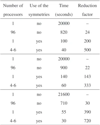
not using the symmetries, the computation times of the nanowire, the slab and the sphere are about 820, 900
and 710 seconds, respectively (See Fig. 10 and Table 1).
Hence, the reduction factors due to the parallelization are between 22 and 30.
6.1. Comparison of Parallelism and Use of the
Symme-tries
Parallelization of the calculations reduces, obviously,
the computation time, but much less than the use of the symmetries. As it has just been indicated above,
par-allel calculations using 96 processors and not using the
symmetries of a nanowire, a slab and a sphere take about
820, 900 and 710 seconds, respectively. Those computa-tion times are longer than the corresponding computacomputa-tion
times of serial calculations using the symmetries: 100,
140 and 55 seconds, respectively (See Table 1). The re-duction factors due to the use of the symmetries are
be-tween 143 and 390, about 6-13 times larger than the
re-duction factors due to the parallelization, which are be-tween 22 and 30 (See Table 1). Therefore, it is much
more efficient (less computation time and also less
com-puter resources) to run serial calculations using the sym-metries than to run parallel calculations without using the
symmetries.
The combination of parallelism and the analysis of the symmetries is also possible. This type of parallel
calcula-tions are based on the parallelization of the algorithm to
calculate the matrix elements and the algorithm to analyze
Table 1: Computation times and reduction factors of the calculations of a nanowire of radius 19a(up), a slab of 2600 atomic layers (center) and
a sphere of radius 5.2a(down), a=3.52 Å, as a function of the number of processors and the use of the symmetries.
Number of Use of the Time Reduction
processors symmetries (seconds) factor
1 no 20000 –
96 no 820 24
1 yes 100 200
4-6 yes 40 500
1 no 20000 –
96 no 900 22
1 yes 140 143
4-6 yes 60 333
1 no 21600 –
96 no 710 30
1 yes 55 390
4-6 yes 30 720
the symmetries. The parallel version of the calculation of
the matrix elements distributes evenly these calculations
among the processors. The parallel version of the analysis of the symmetries also distributes evenly the calculations,
but it is more complex.
As it was explained before, the serial algorithm to an-alyze the symmetries of the magnetic system consists on
a conditioned comparison of the pairs of vectors~ri−~rj
satisfy some of the symmetries or conditions are not com-pared anymore. The parallel version of that algorithm
dis-tributes the comparisons of the vectors as follows. Each
processor comparesa=nv/pvectors, wherenvis the
to-tal number of vectors~ri−~rjthat will be compared andpis
the number of processors. Processorkcompares the
vec-tors from 1+aktoa(k+1)−1. The indexkruns from 0 to
p−1. The last processor,k=p−1, runs from 1+(p−1)a
tonv. Finally, the master node gathers the results.
The parallel algorithm to analyze the symmetries is an
O(N3/p) algorithm. It reduces in an important amount
the computation time of the analysis, but with a price:
The result of the parallel version of the algorithm to an-alyze the symmetries is that the total number of matrices
Mpthat should calculated using pprocessors is
approxi-mately equal to pN, whereNis the number of atoms, if
the magnetic system satisfies the conditions and symme-tries. In a serial calculation, the number of matrices that
should be calculated is approximatelyN. The number of
matrices that should be calculated,Mp, is therefore, larger
than in a serial calculation, although of the same order of
magnitude.
This increase of the number of matrices that should be
calculated has not an important impact on the
computa-tion time to calculate the matrix elements, because the
calculation of the matrix elements is anO(Mp/p)=O(N)
task in a parallel calculation, the same as in a serial
cal-culation. Hence, the result of the parallelization of both
algorithms is an important reduction of the total
computa-tion time, compared with the other types of calculacomputa-tions, as can be noticed in Table 1.
Parallel calculations of the nanowire, slab and sphere
take about 40, 60 and 30 seconds, respectively, using be-tween four and six processors and the symmetries, and
about 100, 140 and 55 seconds, respectively, using one
processor (a serial calculation) and the symmetries (See
Table 1). The parallel calculations with 4-6 processors are the optimal ones: Calculations with a larger or a smaller
number of processors take longer. These calculations with
4-6 processors are about two times faster than the serial calculations using the symmetries.
6.2. Comparison with the Amdahl law
The dependence of the computation time of the calcu-lation of the MDE, not using the analysis of the
symme-tries, on the number pof processors has been compared
with the Amdahl law [49]. This law states that the time of a calculation usingpprocessors is given by:
Tp=
Ts(1+(p−1)s)
p , (33)
where sis between 0 and 1 and is the proportion of the
code that remains serial, because is not parallelized or can
not be parallelized, andTsis the time of a calculation with
one processor (serial run). The results of the parallel
cal-culations of the nanowire, the slab and the sphere have been fitted to the Amdahl law, Eq. 33, obtaining a value
ofsequal to 0.005, 0.007 and 0.008 for the nanowire, slab
as solid lines in Fig. 10. These values of smeans that a
0.5-0.8 % of the code is serial and a 99.5-99.2 % is
paral-lelized.
According to the Amdahl law,Tpshould be about 300
seconds for the nanowire, slab and sphere, using 96 pro-cessors. However, the computation time using 96
proces-sors is 820, 900 and 710 seconds, respectively (See
Ta-ble 1). This is an expected behaviour: The predictions of the Amdahl law are not at all correct for large values of
p. This can be better noticed in the plots of the speedup,
Ts/Tp, of the parallel calculations of the nanowire, slab
and sphere in Fig. 11.
The real speedup matches very well the speedup
pre-dicted by the Amdahl law for p <= 20, but it deviates
largely from the predictions for p > 20. The speedup is approximately constant above p > 20. This is the
expected behaviour of the speedup when the size of the
problem is relatively small. In the present case, the size of the problem is the number N of magnetic moments,
which is about 5000 for the studied nanowire, slab and
sphere. Larger values ofNwill improve the real speedup.
Finally, it should be considered that the basis atoms or magnetic moments of a periodic cell could be such that
their position coordinates do not satisfy the conditions
or symmetries explained in section 3 of this paper. In
that case, the whole periodic system (lattice cell + ba-sis atoms) would be a low symmetry system. If the
peri-odic magnetic system has a low symmetry, then the use of
the symmetries does not reduce the number of matrix
ele-0 12 24 36 48 60 72 84 96
Number of processors 0
10 20 30 40 50 60 70
Speedup = T
s
/Tp
No symmetries used Amdahl law s=0.005
0 12 24 36 48 60 72 84 96
Number of processors 0
10 20 30 40 50 60 70
Speedup = T
s
/Tp
No symmetries used Amdahl law s=0.007
0 12 24 36 48 60 72 84 96
Number of processors 0
10 20 30 40 50 60 70
Speedup = T
s
/Tp
No symmetries used Amdahl law s=0.008
Figure 11: Speedup vs number of processors of the calculations of the following periodic magnetic systems, not using the symmetries: A Ni fcc nanowire of radius 19a, a Ni fcc slab of 2600 atomic layers and a