Assessing policy options for the EU Cohesion Policy
2014-2020
Andries Brandsma *, Francesco Di Comite *, Olga Diukanova *, d’Artis Kancs *, Jesús López Rodríguez *, Damiaan Persyn * and Lesley Potters *
ABSTRACT: In this paper we analyse the possible impact of Cohesion
Poli-cy 2014-2020, putting together the investments supported by EU funding in all NUTS2 regions and running a set of simulations. We make use of RHOMOLO, a spatial CGE model tailored for economic analysis at the subnational level, which is described in the paper. We do so by first considering infrastructure investment, hu-man capital development and innovation climate support, including environmental amelioration, separately and then run a combined simulation of the three catego-ries to give an impression of the pattern and time profile of the overall effect. The results of the simulation show substantial heterogeneity in the effects across the regions, which are not a mere image of the differences in input. The concentration of EU funding on the less developed regions, and on energy saving, innovation and social inclusion in the more developed regions receiving support, could be a fruitful mix for lifting the standards of living in the whole of Europe.
JEL Classification: R13; R58; H54; O32.
Keywords: RHOMOLO; multiregional spatial CGE; Cohesion Policy.
Evaluación del impacto de la Política de Cohesión de la UE 2014-2020
RESUMEn: En este trabajo analizamos el posible impacto de la Política de
Co-hesión de la UE 2014-2020, teniendo en cuenta todas las inversiones financiadas con los fondos estructurales europeos en el conjunto de las regiones NUSTS2 de la UE y simulando un conjunto de perturbaciones. Para ello se usa el modelo RHO-MOLO, un modelo espacial de EGC que está diseñado para el análisis económico
Received: 06 january 2014 / Accepted: 16 september 2014. * European Commission, DG JRC-IPTS.
a nivel subnacional. El conjunto de simulaciones considera primero y de forma separada los impactos de las inversiones en infraestructura, capital humano y el apoyo a los temas de innovación incluyendo las mejoras medioambientales. En una segunda fase se realiza una simulación conjunta de las tres categorías de gasto para tener una impresión del patrón y del perfil temporal de los efectos totales. Los resultados de la simulación muestran una sustancial heterogeneidad en cuanto a los efectos en las distintas regiones, los cuales no son una mera imagen de las diferencias en términos de inputs. La concentración de la financiación de la UE en las regiones menos desarrolladas, y en ahorro energético, innovación e inclusión social en las regiones más desarrolladas podría ser una mezcla exitosa para elevar los niveles de vida en el conjunto de Europa.
Clasificación JEL: R13; R58; H54; O32.
Palabras clave: RHOMOLO; EGC multirregional y espacial; Política de Cohe-sión.
1. Introduction
Greater scrutiny over the performance of Member States and regions benefiting from the European Structural and Investment Funds (ESIF) is part of the design of the EU cohesion policy for 2014-2020, distinguishing it from previous rounds. This goes together with concentration of funding on 11 main lines of support and, geographi-cally, on the less developed among the 271 regions. Each region is expected to have a strategy for using the funds, identifying both the starting point and the potential for economic and social development, and indicating the region-specific targets that have been set. Quantification is essential and required. In principle, funds could be with-held, or the allocation for the next period lowered, when these conditions are not met. This paper presents the spatial computable general equilibrium (CGE) model that has been developed by the European Commission for assessing the impact of the regional policy choices, taken together rather than individually. The main purpose of the paper is to show the pattern of impacts across the regions for the two broad options of investing in the infrastructure connecting the regions and investing in the economic potential of the less developed regions. Although this can be refined to simulate the impact of the more detailed policy choices of individual regions, it will remain problematic to establish, ex post, to what extent a deviation from the targeted impacts is caused by not implementing the policies as intended and to what extent by external effects beyond the control of the region concerned, including those induced by the strategies of other regions.
which makes evaluating cohesion policy so difficult. In their own right, the number of regions and the challenges to multilevel governance do not constitute convincing arguments for modelling. What needs to be captured foremost is the high degree of interdependency between the deepening of economic integration and the increased potential of the regions to benefit from integration.
From its inception in 1988, EU cohesion policy has been accompanied by a growing literature, concerned with the process and its evaluation 1. The most recent
overview is in Bachtler, Méndez and Wishlade (2013). Their analysis challenges the view that cohesion funding is just another battleground for Member States fighting over EU spending. Earlier rounds of cohesion policy are covered in volumes edited by Cuadrado and Parellada (2002), Bachtler and Wren (2006), Cuadrado and Marcos (2005) and Garrido et al. (2007).
In the absence of a regional model, the Commission has had to rely on mac-roeconomic and multi-sector models for its assessment of the impact of cohesion policy. The use of the QUEST III endogenous R&D model is set out in Varga and In’t Veld (2011). This is the Commission’s in-house dynamic general equilibrium model linking the economies of the Member States and the rest of the world, but no deeper than at the national level. Economic development may be reflected by the sectoral composition of national output. In order to capture the sectoral shift induced by re-gional policy the Commission has made use of the HERMIN model for a subset of the Member States (Bradley et al., 2003). The analysis is laid out in Gakova, Grigo-nyte and Monfort (2009), also considering possible extensions to a system of models at sub-national level. In essence, after taking into account conceptual difficulties and computational limitations, this has led to the construction of the spatial CGE model at NUTS2 level presented in this paper 2.
The current version of RHOMOLO covers 267 NUTS2 regions of the EU27 3,
with total production divided into six sectors. Goods and services from home and abroad, that is to say other regions within the same country and (the regions of) oth-er countries, are consumed by households, govoth-ernment and firms. The households in each region receive income from labour, capital and transfers. The geographic interrelations between pairs of regions are obtained through a matrix of asymmetric bilateral transport costs for trade between regions derived from the transport model TRANSTOOLS (Burgess et al., 2008; Petersen et al., 2009).
The CGE approach allows for the interaction between regions to be captured within a fully consistent framework solving for simultaneous equilibrium in the goods, services and factor markets, but may run into computational limitations if the number of regions and sectors becomes very large. It therefore needs to be imposed
1 For more information on the evaluation of past Cohesion Policy measures and on the future and
on the strategies and plans for the next programming period, see the Sixth report on economic, social and territorial cohesion (European Commission, 2014).
2 Ferrara, A., Ivanova, O. and Kancs, D. (2010) provide a formal description of the prototype. 3 The full inclusion of the two Croatian regions is waiting for the data to become available. The
that each sector produces just one composite good and the usual Dixit-Stiglitz and Armington assumptions are made to keep the system of equations manageable. More fundamentally, although the model is derived from optimization by representative economic agents, forward-looking expectations consistent with model outcomes can-not be handled within the current set-up. Bradley (2006) already recognised the chal-lenge of reconciling bottom-up micro-analysis with top-down macro-analysis. The approach taken in this paper is to align the RHOMOLO results with the aggregate impact generated with QUEST under model-consistent expectations. To the extent possible the two models are made to share the microeconomic foundations, whereas the rich dynamics of the QUEST III endogenous R&D model are superimposed on the sequence of solutions over time of the spatial CGE model.
The paper is organised as follows. First, Section 2 provides some further back-ground on EU cohesion policy and the changes that are envisaged. Section 3 gives a brief technical description of RHOMOLO, touching upon its structure, characteris-tics and dynamics. Section 4 describes in detail the design of the four main scenar-ios that have been simulated (Human Capital, R&D, Non-R&D and Infrastructure investments) and Section 5 presents the outcomes of these simulations as deviations from the baseline without cohesion policy interventions. Finally, Section 6 con-cludes.
2. Concentration of funding under EU cohesion policy
EU cohesion policy has its roots in the Treaty of Rome, but it was on the waves of the single market and the European Union’s enlargement that the policy got its present size and shape. All together, the ESIF are the second largest comprehensive part of the EU budget, absorbing roughly one third of the expenditure 4.
The ESIF are three different funds with their own objectives and stakeholders: — The Cohesion Fund available to Member States with a GDP per capita of
less than 90% of the EU average supports investment aimed at fulfilling the convergence objective. Its main activities are directed at improving the trans-European transport (TEN-T) networks and the environment, notably in the fields of energy or transport (e.g., supporting energy efficiency, the use of renewables, public transport, inter-modality);
— The European Social Fund (ESF) is the EU’s main financial instrument for investing in people. It increases the employment opportunities of European citizens, promotes better education and helps containing the risk of pover-ty. The ESF covers measures aimed at fostering lifelong learning schemes, reducing search and matching costs in the labour market, promoting social
4 There are two additional funds that fall under the Commission’s Common Strategic Framework:
integration, combating discrimination and strengthening human capital by reforming education systems;
— The European Regional Development Fund (ERDF) aims to strengthen eco-nomic, social and territorial cohesion in the EU by correcting imbalances between regions. The ERDF supports regional and local development, in-cluding actions in the field of sustainable urban development.
The combination of the Structural Funds (ESF and ERDF) and the Cohesion Fund amounted to 347 billion euros, equivalent to roughly 0.3% of EU-27 GDP, in the programming period 2007-2013. For individual regions, the financial support can be as high as 4% to 5% of their GDP. The support is provided under the principles of additionality and partnership. Concentration and multi-annual programming are the tools for aligning the use of the funds to EU objectives and priorities. Additionality refers to the requirement that contributions from the structural and cohesion funds are not simply substituted for national expenditures already planned. Partnership re-quires a collective process involving authorities at European, regional and local level, social partners and organisations from civil society 5.
The funds are the EU’s instruments for channelling the contributions of the Member States into investments in infrastructure, people and the environment, pri-marily through financial support provided at the regional level. In the words of the Treaty of Lisbon, in order to promote its overall harmonious development, the Union shall develop and pursue its actions leading to the strengthening of its economic, so-cial and territorial cohesion. The Union aims at reducing disparities between regions with a particular focus on the backwardness of the least favoured regions.
2.1. How to model EU cohesion policy
Over the years, the emphasis of cohesion policy has shifted from an attempt to shield the countries and regions from the consequences of fiercer competition within the single market to a strategy of enhancing the potential of the regions to take greater advantage of European integration. What this means for the approach followed in this paper is that RHOMOLO should be able to capture both the lowering of barriers between regions, reflected in shifts in inter-regional and cross-border trade, and the increased potential of the regions resulting from the access to the ESIF. The model is set up to deal with the broad strokes of policies to stimulate growth, employment and competitiveness at the regional level, rather than the detailed channels of financial support of the structural and cohesion funds.
RHOMOLO as it stands has three major handles for putting in the interventions under cohesion policy:
— the reduction of transport cost resulting from the investment in infrastructure, differentiated for the bilateral connections between each pair of regions;
5 See http://ec.europa.eu/regional_policy/index_en.cfm for more detailed information about
— the shifts in labour productivity resulting from the investments in human cap-ital, which have a distinct profile with highly positive effects in the long term and possibly negative in the short run; and
— the improvement in total factor productivity, outside the labour-capital bun-dle, which represents technical progress and innovation among other factors behind regional economic growth.
In addition, it would be possible to assign some interventions to sectors of economic activity and to use the cost of newly built-up physical capital as a pa-rameter. For instance, the sector of construction may benefit heavily from partic-ular investments in infrastructure. However, it is far from obvious in which region the companies benefiting from such investments would be located. The demand effects in the simulations of this paper are therefore left to the inner workings of the model, including the input-output relations embedded in the production structure.
Table 1 shows the result of grouping the lines of expenditure into macro catego-ries for the purpose of the simulations.
Table 1. Details on Cohesion Policy expenditures (in € millions). GDP values are reported for 2007 because that is the year used for the calibration
of the model due to data availability at the regional level
Region type1 # GDP 2010 RTDI
Aid to private sector
Infras-tructure
Human Capital
Techni-cal Assis-tance
Total %
Less Developed
Regions 65 1,199,595 25,250 27,127 129,128 38,408 12,162 232,075 68 Transition Regions 51 1,466,019 5,772 6,218 14,339 10,201 1,585 38,115 11 More Developed
Regions 151 9,539,148 10,916 9,101 24,167 24,196 2,954 71,335 21 Total 2672 12,204,762 41,938 42,447 167,634 72,805 16,701 341,525 100
% of total CP 12% 12% 49% 21% 5% 100%
1 The less developed regions have a GDP per capita that is less than 75% of the EU-27 average. The GDP per capita of the transition regions
is between 75% and 90% of the EU-27 average and for the more developed regions this is above 90%.
2 The EU27 has a total of 271 NUTS2 regions, but 4 French regions are left out because of their very particular characteristics: Guadalupe,
Martinique, Guyana and Réunion. The two Croatian regions are not included yet because of limited data availability.
Funding for Research, Technical Development and Innovation (RTDI) is aimed at supporting firms with the uptake of novel research findings in the actual imple-mentation of innovations. The RTDI related expenditures are assumed to affect the innovation capacity of the economy, which is translated into changes in the total factor productivity (TFP) parameter of the model. Section 4.2 discusses the set-up of the TFP simulations in greater detail.
The category Aid to Private Sector covers support to activities that are not im-mediately associated with R&D. They nevertheless can play an important role in the economic development of countries and regions that are at a considerable distance from the technology frontier by easing the way towards that frontier and raising
TFP. These non-R&D innovation activities consist e.g. of technology and know-how acquisitions, such as machinery and other equipment patents, trademarks, designs, etc. In Europe, about 40-60% of the industrial value-added and 50% of all industrial employees are engaged in the non-R&D intensive sector (Som, 2012). Moreover, more than half of all innovating firms in the EU are non-R&D performers (Arundel
et al., 2008). Therefore, considering the high shares of funding devoted to the
non-R&D activities and the importance of these activities in the promotion of innovation and TFP growth in Europe, it is important to evaluate the ex-ante effects of the planned regional non-R&D investments across EU regions. More details are provid-ed in Section 4.3.
Funds aimed at investment in Infrastructure mainly support regions in im-proving connectivity within the region and with other regions. The main focus is on railways, motorways and airports, as well as on improving the environmental and social infrastructure of the regions. The investments can be expected to lead to a decrease in transport costs, as well as in the general cost for doing business. For instance, they may lower the cost of communication, making it easier to sell final goods or source intermediates. These investments will be modelled as a reduction of the transport costs. The setup is discussed more in detail in Sec-tion 4.4 6.
The envelope is spread over the years based on the experience of past Com-munity Support Frameworks. In addition, the N+3 rule 7 is applied, so that the ex-penditures run from 2014 to 2023. The assumed time profile is shown in Figure 1. The same profile applies to all regions and they are expected to be able to increase their absorption capacity as compared to the 2007-2013 programming period. It is assumed that by 2018 more than 50% of the allocated funds will have been spent and up to 80% by 2020.
6 Given its relatively small size in the overall budget and the difficulty to model it in a consistent
way, the category Technical Assistance has not been modelled. It mostly concerns technical support pro-vided to regions or local authorities for streamlining bureaucratic procedures, public programming and auditing.
7 The Commission shall automatically «decommit» any part of a commitment which has not been
Figure 1. Time Profile of Cohesion Policy expenditures
100 90 80 70 60 50 40 30 20 10 0
(%
)
Cumulative Cohesion Policy Expenditures (% of total)
2014 2015 2016 2017 2018 2019 2020 2021 2022 2023
2.2. The main themes of EU cohesion policy for 2014-2020
The 2014-2020 round of cohesion policy is characterised by a concentration of funding, geographically as well as thematic. It mirrors closely the EU 2020 objec-tives with their focus on sustainable growth, creating jobs within an inclusive society. In comparison with the previous round, the number of lines of expenditure under which structural and cohesion funding is spent has been concatenated, partly revers-ing the proliferation of projects. The eleven thematic objectives for deliverrevers-ing Europe 2020 through ESIF are:
1. Strengthening research, technological development and innovation. 2. Enhancing access to, and use and quality of, information and
communica-tion technologies.
3. Enhancing the competitiveness of small and medium-sized enterprises, the agricultural sector and the fisheries and aquaculture sector.
4. Supporting the shift towards a low-carbon economy in all sectors. 5. Promoting climate change adaptation, risk prevention and management. 6. Protecting the environment and promoting resource efficiency.
7. Promoting sustainable transport and removing bottlenecks in key network infrastructures.
8. Promoting employment and supporting labour mobility. 9. Promoting social inclusion and combating poverty. 10. Investing in education, skills and lifelong learning.
fa-voured regions. Themes 4-6 are directed at making the European economy more resource efficient —less energy dependent— and contributing to climate change tar-gets. Regions may learn some lessons on best practices from one another and from light competition on environmental attractiveness between them, but air pollution and global warming are not contained within regional borders and typically need to be sorted out at the supranational level. The use of structural and cohesion funds for environmental purposes is mostly related to urban development, nature, water and waste. Other themes —focusing on research and innovation (1), ICT (2), transport (7) and mobility (8)— have as much to do with the interconnection of regions as with remedying their backwardness, and assigning them to the regions, as in Table 1, is somewhat arbitrary.
From a modelling point of view, there would be no need to have a full allocation of funds to the regions. The model itself generates the regional distribution of the returns on the investment, some of which will be tied to the region and another part to the connections between the regions. This is in fact the way it has been implemented in RHOMOLO for the purpose of the exercises in this paper. The budget for cohesion policy post-2013 amounts to 380 billion euros in total, including 40 billion euros for the Connecting Europe facility for transport, energy and ICT. The latter is clearly spent on the networks connecting the regions and is modelled through a reduction in transport costs which is estimated with the help of the TRANSTOOLS model using detailed data on the TEN-T investments in roads, rail and waterways.
For the 2014-2020 period, the Cohesion Fund is dedicated to investment in cli-mate change adaptation, energy saving and risk prevention in Bulgaria, Croatia, Cyprus, the Czech Republic, Estonia, Greece, Hungary, Latvia, Lithuania, Malta, Poland, Portugal, Romania, Slovakia and Slovenia. Some 10 of the nearly 70 billion euros reserved for the Fund are ring-fenced for the Connecting Europe facility. All in all, the broad thematic decomposition in Table 1 shows that nearly half of the ESIF can be attributed to investment in infrastructure, not counting the 40 billion for the facility itself.
The other half of the ESIF is spent on education and training, that is investing in human capital, and support to research and innovation in enterprises, including SMEs in the regions. Relatively little goes to R&D activities proper; the category Aid to the private sector consists of such things as financial support for acquiring new equip-ment and know-how and for applying for patents, trademarks and designs with local/ regional content. It is envisaged that part of the ESIF may be dedicated to assisting researchers in Horizon 2020 participation and providing enterprises with easier ac-cess to the results of earlier Framework Programs, mainly to the benefit of countries that joined the EU since 2004.
recently, either of their own account or because the EU average fell as a result of the recent enlargements.
2.3. The 2014-2020 allocation of funding
It is interesting to consider the matrix of thematic and geographical allocation from a political angle. Bachtler and Méndez (2007) made a careful assessment of the governance of EU cohesion policy at the start of the 2007-2013 round. They argue that the doubling of the funding in 1988 accompanying the single market initiative has been followed by largely unsuccessful attempts, at each review and renegotiation of the allocation and spending, to shift the decision power on the spending of the structural funds back to the Member States. In terms of geographical allocation, half of the funding continues to go directly to the less developed regions. The battle is mainly over the remaining part of the structural funds, and in particular the European Social Fund (ESF). On the proposal of the Commission, maximum co-financing rates have been set, which range from 50% for the most developed regions to 85% covered by the EU contribution from the Cohesion Fund. Some of these rates have been in-creased in response to the economic and financial crisis.
The Commission has raised its leverage even further by setting minimum shares for categories of spending under each Fund. For example, under the ERDF, at least 80% of the spending in the more developed and transition regions, aggregated by Member State, should be devoted to the use of natural resources, innovation and SME support. At least one quarter of this is expected to go to energy efficiency im-provements and renewables. Less developed regions have greater leeway in setting investment priorities, reflecting more diverse needs in catching up with EU average standards, but will have to spend at least 50% of ERDF resources on energy saving, innovation and SME support.
Minimum shares have also been established for the use of ESF support as a per-centage of total EU funding: 25% for the less developed regions; 40% for the regions in transition; and 52% for the more developed regions. The upshot of all this is that the bulk of the ESIF is going to the least favoured regions, with investment in infra-structure and human capital as the two biggest categories. More developed regions receiving support are very much restricted in their use of the funds, which should be spent mostly on promoting energy efficiency and innovation and enhancing job opportunities and social inclusion.
point of time, after the mid-term review has taken place. Failure to reach the targets agreed with the Member State concerned and fulfil the requirements may lead to the suspension or cancellation of EU funding.
3. Brief description of RHOMOLO
The RHOMOLO model is calibrated to the regionalised Social Accounting Matrices (SAMs) of the EU member states that were extracted from the World In-put-Output Database (Timmer, 2012). SAMs for the NUTS2 regions were construct-ed using the data of regional production by sector, bilateral trade flows among the NUTS2 regions, and trade with the rest of the world (ROW), as described by Potters
et al. (2013). The version of the model used for this paper includes 6 NACE 8 Rev. 1.1
industries: Agriculture (AB), Manufacturing (CDE), Construction (F), Transport (GHI), Financial Services (JK) and Non-market Services (LMNOP).
EU regions are modelled as small open economies that accept EU and non-EU prices as given, which is consistent with the regional scope of the model. In this perspective, EU external relations involve only one non-EU trading partner that is represented by the ROW aggregate
Interregional trade flows are estimated based on prior information derived from the Dutch PBL dataset (Thissen et al., 2013). Data on bilateral transport costs per sector are provided externally by the TRANSTOOLS model 9, a model
covering freight and passenger movements around Europe. The costs of different shipments are calculated in terms of share of the value shipped, based on the time needed to reach the destination using alternative modes of transport. Transport costs thus differ by type of good and depend on the distance between the regions and the variety and characteristics of modes of transport connecting them, which also means that they can be asymmetric. The representation of trade and transport flows among the NUTS2 regions gives the model a spatial dimension, indicating that EU regions differ not only in their stocks of production factors but also in geographic location.
Mobility of capital and labour is assumed to occur within regions, but interna-tional or intra-regional migration of production factors is not considered in the core model version.
All agents of the model are assumed to have myopic expectations and do not anticipate future changes in relative prices or make choice between consumption and savings depending on the interest rate. Using a perpetual inventory method (OECD, 2001), the sum of interest rate and depreciation rate are employed to estimate the regions’ capital stocks from the value of their operating surplus, as available in the SAMs. The interest rate is set at the level of 5% and the capital depreciation rate at
8 See http://epp.eurostat.ec.europa.eu/statistics_explained/index.php/Glossary:NACE.
6% per annum 10. In order to keep the model baseline «clean» of trade spillovers that
change relative prices and induce sectorial changes, we apply a uniform 2% annual growth rate to all regions.
The model solves for the sequence of equilibrium states when all time periods are connected with the equation of capital accumulation: each year in each region a portion of capital stock depreciates and gets augmented by the previous year in-vestments, so that capital stock and investments grow at the same rate with the rest of economy. Values of investments in each region are adjusted in order to achieve consistency among the observed investments, the estimated capital stock and the re-quired replenishment of the capital stock. Therefore, there are no changes in regions’ economic structures over the steady-state baseline period. All prices remain constant; only the quantities grow at the same constant rate. This enables the comparison of the after-shock results with the baseline values 11.
3.1. Composite of domestic and imported varieties
Domestically produced and imported varieties are combined with a CES func-tion. Trade and transport margins are applied to imports from other NUTS2 regions and to domestic sales (ttm). Following this specification, the structure of composite good is depicted in Figure 2.
Figure 2. Composite of domestically produced and imported varieties of the same good
Imports
Imports from the region UKN0
…
CES Composite good
ttm ttm
Imports from the ROW Imports from
the region AT11 Domestic
sales
ttm
Composite goods are consumed by industries, households, government, and the investment sector.
10 In reality, interest rates may change over time, but for modelling standard values are assumed in
the literature.
11 The core model equations are specified in the calibrated share format proposed by Rutherford
3.2. Industries’ nested cost function
In a core model version the CET function defines the sectors’ choice between sales on the domestic market and exports to other regions as function of relative prices on these markets. However, in order to introduce imperfect competition, the CET function has to be removed. Taking into account that sectors’ export sup-ply to the NUTS2 regions is determined by import demand of these regions (see Figure 2), we can dismiss the constant elasticity of transformation (CET) function of output transformation to regional markets. However, the aggregate of non-EU economies (ROW) cannot be treated as one of model’s regions. Even though a SAM for ROW can be constructed using a GTAP database (Badri Narayanan et al., 2012), adding the ROW region to a RHOMOLO would create computational difficulties, as model would be calibrated to the SAMS of 270 small regions that have relatively small values of economic transactions and one ROW region with large values. Hence, following the approach of Whalley and Yeung (1984), export supply to the ROW is modelled with a function of export demand from the Rest of the World.
A Leontief function is employed on the top level of the sectors’ production func-tions in order to define complementarity between the intermediate inputs and the labour-capital aggregate. The lower level of the sector’s production function features the possibilities of trade-offs between labour and capital services that were specified with the CES function; intermediate inputs are assumed to be non-substitutable. Co-efficients of factor productivity improvements are assigned to labour (fpl) and capital (fpk). With this specification, producers can maintain the same levels of output using less production factors. The same structure of nested production functions is adopted for all sectors (see Figure 3).
Figure 3. Sector’s nested production function
Exports
Exports to the ROW Domestic
sales
…
CET
tc
Lt
CES
Labour Capital
tl tk
LMNOP
JK
GHI F CDE
AB fpk
fpl Labour-capital
aggregate Exports to the
3.3. Budget balance and structure of household consumption
According to the information, which was provided in the regional SAMs, re-gional households supply labour and capital services, pay income taxes, receive net transfers from the public sector, and also net transfers from abroad. Households save a fixed proportion of their income.
After deducting taxes, transfers and savings, the disposable income is used to maximize utility of households’ consumption. The final goods that are consumed by households are combined, allowing for substitutability among inputs. The structure of regional household consumption is described in Figure 4.
Figure 4. Structure of regional household expenditures and public expenditures
Household consumption
LMNOP CD
JK GHI
F CDE
AB
3.4. Budget balance and structure of Public consumption
According to the SAMs, income of regional government consists of taxes on sec-tors’ output, secsec-tors’ consumption of labour, capital services, taxes on regional invest-ment good, income taxes, net transfers from abroad and net transfers from regional households. In the model we assume fixed tax rates and constant public consumption of final goods. Hence, public savings are determined as a residual.
The structure of regional public consumption was specified in a similar manner to that of households (Figure 4).
3.5. Savings-investment balance
3.6. Market clearing conditions
Since model is formulated in a calibrated share format, demand and supply of goods were defined by differentiating the profit or cost function by the price of that good (Hotelling’s and Shephard’s lemmas).
3.7. ROW closure
Following the (small open economy) SOE assumptions, any of the NUTS2 re-gions doesn’t influence prices in the non-EU market. Therefore, we formulated the EU balance of trade as net exports to the ROW. We fix the ROW savings keeping the real exchange rate flexible, so that ROW price adjusts to bring about equilibrium. Savings from the EU are set exogenously and valued using a producer price index
4. Scenario construction
4.1. Human capital related policies
The budget line Human Capital under cohesion policy covers a wide variety of expenditures. Some aim at fostering re-integration of long-run unemployed on the labour market, while others pertain to improving life-long learning or on the job training. To simulate the effects of cohesion policy on human capital in RHOMOLO, the expenditures are aggregated into a single exogenous shock by assuming that they all lead to an increase in regional labour productivity (the fpl parameter), at the cost of a temporary decrease in the local labour supply.
Next, it needs to be specified how efficient the policy is in improving regional labour productivity. For this, it is assumed that the percentage increase in the human capital stock of the region induced by cohesion policy equals cohesion expenditure on human capital relative to the total expenditure on education in the region, taken from EU KLEMS (Timmer et al., 2007). Next, in accordance with the estimates in the empirical literature, it is assumed that increasing the stock of human capital by 1% leads to an increase of 0.3% in output per worker (Sianesi and Van Reenen, 2003). In the initial years of the policy implementation, labour supply simultaneously is assumed to decrease and remains subdued during the programming period. After the programming period, labour supply recovers to its original level.
4.2. R&D investments
For the 2014-2023 period, 42 billion euros have been allocated to lines of expen-diture related to support to RTDI. This is 12% of the grand total of Cohesion Policy funds; 60% of this goes to the less developed regions, a lower percentage than the 70% across all budget lines.
In order to depart from a framework with simplified growth dynamics à la Solow (1956), the current version of RHOMOLO introduces an endogenous growth mecha-nism à la Howitt (2000). López-Bazo and Manca (2014) use a specification in which
TFP growth is determined by a combination of RTDI investment and catching up with other regions. There is considerable empirical evidence of the effect of R&D
on TFP, very well elaborated in Hall et al. (2009). The investment in RTDI under cohesion policy is first expressed as an increase in the R&D intensity compared to the baseline and subsequently a TFP equation is used to model the increase in TFP re-sulting from R&D. This is the most standard formulation derived in Hall et al. (2009) which is reproduced here in a distributed lag format, reflecting that it takes time for an investment in R&D to be turned into innovation and consequently a productivity improvement. The TFP equation is as follows:
TFP TFP
b b RTDI
reg t reg t
re , * , ( )* * * = + − + −
γ 1 γ
0 1 1 gg t reg t reg t reg t GDP b RTDI GDP T , , , , , , * *
sec + sec
2 FFPgapreg reg t, , * b TFP* t
( ) + 3 1 elsewhere
where TFPregrepresents the level of regional TFP at a given point of time that
sub-sequently has an impact on the total output. The term RTDI
GDP
reg
reg
,sec
is the R&D
inten-sity for each sector in each region. The second explanatory variable is the combined interaction between the average R&D intensity and the gap in TFP with the leading region. It should be noted that the further away is the region from the technology frontier the faster it will catch up given the same R&D intensity. This is because there is a greater potential for closing the gap by borrowing from the existing stock of knowledge and know-how.
The third term between brackets represents possible spillovers from TFP increases in other regions and sectors (TFPelsewhere). These spillovers are the key reason why the social return on R&D exceeds the private return, and thereby would justify public investment and support to R&D in the private sector. This is a topic of empirical research taken up by Belderbos and Mohnen (2013), who propose a patent citation-based indica-tor to measure the presence of intra- and inter-secindica-toral knowledge spillovers, nationally as well as cross-border. This could possibly at a future stage be transformed into a spatial structure for the spillovers between regions but for the moment b3 is set to zero.
the 20% to 30% range. This estimate is introduced in the model by setting a rate of return. This is close to the estimate used in QUEST III (McMorrow and Röger, 2009).
The empirical evidence on the spillover effect and catching-up is not as strong, but it is likely that the farther away from the technology frontier the greater the po-tential for catching up, conditional on the ratio of R&D to GDP. This is introduced in the model by a multiplicative term expressing that the higher the R&D intensity the greater the part of the TFP gap that is closed every year. An increase in RTDI ex-penditure compared to the baseline will set in motion this process, which is assumed to operate with the same distributed time lag and coefficient as the R&D effect on its own. This would approximate a doubling of the rate of return on RTDI for regions which are TFP =1 at compared to the technology frontier (TFP =2) 12. The estimates
behind this specification are confirmed by the econometric research of López-Bazo and Manca (2013).
4.3. Support to innovation other than through R&D
Innovation can take place through activities which do not require R&D such as the purchase of advanced machinery, patents and licenses, training related to the in-troduction of new products or processes, etc. These forms of acquiring knowledge and technology are referred to here as non-R&D (NR&D) innovation activities. From a policymaking point of view, it is important to analyse the impact of NR&D mea-sures since a sizable portion of the cohesion policy budget is devoted to such support. In the 2014-2020 round, some 40 billion euros are devoted to NR&D activities. The current version of RHOMOLO analyses its impact considering that the main channel of influence of these activities is through their impact on TFP. López-Rodríguez and Martínez (2014) estimate an elasticity of TFP with respect to the NR&D investments of
(
γ3+γ1Ird)
13. Mathematically, the following expressions have been used toesti-mate the shifts on TFP due to NR&D funds:
gTFP y Ird NR D
GDPbau
reg t
t reg
t re
,
,
, &
=
(
+)
−−
3 1
1
1
γ
gg
reg t reg t reg t
TFP gTFPbau gTFP
= +
( )
, , ,
2
3)) ( )3
where gTFPreg,t is the annual regional growth rate in TFP in region reg in year due to NR&D innovation expenditures; g3 + g1 Ird is the elasticity of TFP improvements
with respect to NR&D investments, taken from López-Rodríguez and Martínez (2014); NR&Dt–1,reg is the amount of NR&D innovation expenditures assigned in the
12 Luxembourg, Brussels and Greater London are excluded from the frontier, because they are
year t – 1; GDPbaut–1,reg is the forecasted GDP region in the year is the baseline an-nual regional TFP growth in the region reg during the year t; TFPreg,t; is the growth rate induced by the NR&D investments.
For the purpose of this exercise not only the values of allocated funds are in-troduced but also the planned annual absorption of non-R&D investments for each region during the compliance period of 2014-2023. It should be noted that regional
NR&D investments are not distributed homogenously in the plans for the period of 2014-2023, but show fluctuations from one year to the next. Given that the model baseline was projected assuming a steady-state 2% annual growth rate, region’s val-ues of TFP growth can double or triple from one year to another.
4.4. Infrastructure investments
In a first step, an aggregate measure of the total expenditure on transport infrastruc-ture under cohesion policy is derived for each region. For this purpose, all policy instru-ments directly affecting transport infrastructure are aggregated in one category, INF 14.
In a second step, an attempt is made to impute the spatial dimension of the trans-port infrastructure funds based on region-specific expenditures as calculated in the first step by estimating how region-specific expenditure translates into region-pair-specif-ic expenditure. The spatial dimension is important, because transport infrastructure improvement affects not only the region in which the investment is made, but also all regions with which it trades goods and services. The following formula is used to impute a spatial matrix of bilateral transport investments, ECPreg reggINF, :
ECPreg reggINF ECP ECP reg regg
reg INF
egg INF
, = ,
+
φ
22 4
( )
where ECPregINF
and ECPrergINF are ECP transport infrastructure expenditures in regions
reg and regg, respectively, and φreg regg, ≡τreg regg1−σ, is the freeness of trade, which
rang-es from zero, when trade is perfectly un-free (bilateral trade costs are prohibitive between reg and regg), to unity, when trade is perfectly free and bilateral trade costs are zero (Baldwin et al.,φ 2005). τ σ
reg regg, ≡ reg regg1−, denotes bilateral trade costs between pairs of
regions as measured by TRANSTOOLS.
The bilateral measure of transport infrastructure investments (4) takes the ex-penditure in the regions at both ends as well as the proximity of the regions into ac-count. The second term on the right-hand side in equation (4) calculates the average transport investment for every pair of regions. The first term on the right-hand side
14 Note that no weights are applied at this stage of aggregation, although, according to the theoretical
introduces a spatial structure (economic geography) in the bilateral measure of trans-port infrastructure investment by weighting the proximity (integration) of regions. The farther away the trading regions are (trade is more costly), the less weight will be attributed to the transport infrastructure improvements between the two regions. The weighting implies that the further away are the two regions, the lower impact will have a fixed amount of expenditure (1 km of road can be improved much better than 10 km of road with the same amount of funds).
In a third step, ECPreg reggINF
, , which is a bilateral measure of expenditures, is
trans-formed into changes in bilateral trade costs between regions, which are measured as a share of trade value. This is done by pre-multiplying the bilateral measure of transport infrastructure investments ECPreg reggINF
,
(
)
by a coefficient measuring the ef-fectiveness of transport infrastructure investments. The elasticity of trade costs with respect to the quality of infrastructure is retrieved from studies on TEN-T infrastruc-ture (European Commission, 2009), since no comparable elasticities are available for Cohesion Policy investments in transport infrastructure. The result is a transport infrastructure scenario that can be readily implemented in the model.5. Simulation results
Given the complexity of interactions and spillovers in RHOMOLO, regional shocks induced by cohesion policy are quickly transmitted across regional and na-tional borders. In fact, EU regions are interconnected through a dense network of trade in goods and services and technology transfers which make the model and the interpretation of its results not easily tractable. In order to fully capture the effects of each expenditure item and the role played by interconnections, the simulated impact of each measure is shown in in isolation and then combined. Following the order proposed in the scenario construction (Section 4), first human-capital related poli-cies are presented below, then R&D investments, followed by non-R&D support and infrastructure investments. Finally, the possible overall impact of cohesion policy is put together in a combined simulation illustrating the extent of spatial interrelations.
5.1. Interventions in the field of Human Capital
Cohesion policy expenditures on human capital are projected to account for about 20% of total cohesion policy expenditures for the 2014-2020 round. To sim-ulate the effects on human capital in RHOMOLO, the expenditures are assumed to lead to an increase in labour productivity, however at the cost of a temporal decrease in the regional labour supply. Formally, an expenditure on human capital of 1% rela-tive to local education expenditures is assumed to increase local labour productivity by 0.3% 15.
Increase in regional labour productivity implies an increase in regional GDP but also an increase in labour demand and wages. The following map displays the yearly average impact of investments in human resources under cohesion policy over the 2014-2023 period.
Map 1. Impact of interventions in the field of human resources on NUTS 2 regions GDP in 2023, % deviation from baseline
(.185, .546) (.023, .085) (.009, .014) (.005, .006) (.003, .004)
HR impact on GDP, yearly average 2014-2023 (.085, .185) (.014, .023) (.006, .009) (.004, .005) (–.025, .003)
As Map 1 suggests, the overall effect of investment in human resources is clearly positive, especially in most of the Central and Eastern European Member States. This reflects the distribution of cohesion policy support which is much higher for the less developed regions than for the transition and more developed regions.
Finally, investment in human resources also generates spatial spillovers. As for infrastructure investments, the increase of GDP in the regions receiving support ben-efits other regions because of the interregional trade links.
5.2. Interventions in the field of R&D
R&D is another key sector of intervention for cohesion policy and accounts for approximately 12% of the total cohesion policy budget (or some 40 billion euros) which is to be allocated to lines of expenditure associated with support to research, technological development and innovation (RTDI) during the 2014-2020 programing period. More than 60% of this is allocated to the less developed regions.
As discussed in Section 4.2, in RHOMOLO support to RTDI is assumed to in-crease TFP. An increase in R&D affects GDP in several ways. First, GDP increases due to the fact that R&D leads to an increase in total factor productivity. This implies a reduction in the prices of intermediate inputs and hence of production costs which also contributes to the increase in GDP. Finally, the price of consumption goods de-creases which encourages demand and hence the level of economic activity. As for other fields of intervention, other regions benefit from a rise in GDP due to increased demand from the regions receiving RTDI support.
The model accounts for spatial spillovers specific to R&D. Formally, it is as-sumed that the farther away a region from the technology frontier, the greater the potential for absorption and imitation of technological progress produced elsewhere. This not only implies that lagging regions are catching up on more advanced ones in terms of technology but also that an increase in R&D produces a bigger impact on factor productivity in regions where the level of technology is originally low.
The results of the simulation show positive effects in all regions, with very few exceptions due to the intensification of competition from catching-up regions (see Map 2). Czech, Hungarian, Polish and Portuguese regions benefit the most, with im-pacts on regional GDP of 1-2% above the baseline on average in the 2013-2023 period. The impact on GDP in the less developed regions on average is somewhat higher than 1.2% on average in the 2014-2023 period. A renewed/continued increase in RTDI would be needed to keep the regional economies on a higher growth path.
In general, the impact is higher in less developed regions than in transition re-gions. This is explained by the fact that less developed regions receive more support under cohesion policy than the two other groups and that R&D investment has a higher impact on TFP in lagging regions in terms of technology.
5.3. Interventions in the field of non-R&D support to innovation
policy. Map 3 shows the average impact of non-R&D measures on GDP across the NUTS2 regions in EU-27 in 2014-2023. The impact on non-R&D support is pos-itive in all regions although their magnitude varies considerably between regions. The most benefiting regions are those located in the Eastern parts of Europe and the Southern European periphery (Greece, Southern Italy, Spain and Portugal). Central European regions are expected to benefit only mildly. The results of the simulations are highly correlated with the amount of non-R&D funds received.
5.4. Interventions in the field of infrastructure
Finally, investments in infrastructure are planned to be nearly 170 billion euros, almost half of the total funding available.
However, there are large differences between regions concerning cohesion policy expenditure on infrastructure. Indeed, larger amounts are allocated to less developed regions. In addition, the share of infrastructure in the allocation is also higher than in more developed regions. Accordingly, cohesion policy expenditures on infrastructure
Map 2. Impact of interventions in the field of R&D on NUTS 2 regions GDP
in 2023, % deviation from baseline
(.23, .788) (.024, .072) (–.002, .009) (–.004, –.003) (–.016, –.006)
R&D impact on GDP, yearly average 2014-2023 (.072, .23)
(.009, .024) (–.003, –.002) (–.006, –.004) (.23, .788)
(.02
(
(
( ( 4, .072) (–.0
( (
(–
( 02, .009) (–.0
( 04, –.003) (–.016, –.006) R&D
R impact on GDG P, yearly average 2014-2023 (.07
(
( 2, .23) (.00
( ( 9, .024) (–.0 (
( 03, –.002) (–.0
( ( (
allocated to the less developed regions are considerably higher than to the transition and more developed regions.
In order to simulate the impact of cohesion policy investment in the field of in-frastructure, the corresponding expenditure needs to be «translated» into changes in some of the model’s parameters. Infrastructure investments are assumed to reduce transport costs between regions and the parameters representing transport costs are adjusted accordingly. Bilateral transport costs can be used to calculate an indicator of each region’s accessibility. There are significant differences in transport cost re-ductions between regions and the largest improvements in accessibility take place in the less developed regions which reflects the expenditure pattern of Cohesion Policy.
Improvement in transport infrastructure means that regions get better connected within the single market which increases their exports and hence boosts the level of economic activity. The lowering of transport costs also implies a reduction in the price of imported intermediate goods and of consumption which contributes to a reduction reduce in firms’ production costs and an increase in the disposable income of households. All these effects lead to an increase in regional GDP in the 2013-2023 period, as shown in Map 4.
Map 3. Impact of interventions in the field of non-R&D on NUTS 2 regions GDP
in 2023, % deviation from baseline
(.06, .13) (.037, .06) (.02, .037) (.007, .02) (0, .007) (–0005, 0)
Map 4. Impact of interventions in the field of infrastructure on NUTS 2 regions
GDP in 2023, % deviation from baseline
(1.741, 2.643) (.289, 1.144) (.053, .117) (.027, .033) (.007, .019)
INF impact on GDP, yearly average 2014-2023
(1.144, 1.741) (.117, .289) (.033, .053) (.019, .027) (.004, .007)
The largest returns on investment in accessibility are found in the less developed regions of the EU. It is in these regions that accessibility is lacking and where trans-port infrastructure has the greatest potential for improvement.
The impact of investment in the field of infrastructure does not only materialise in the regions where the investment takes place. A region benefiting from enhanced accessibility increases its imports of goods from the other regions which in turn also experience an increase in their exports and hence their GDP. The impact of local intervention therefore has a tendency to progressively disseminate in space through the numerous trade links existing between the EU regions.
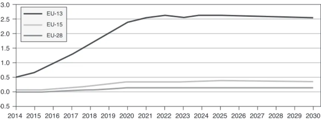
5.5. Simulating Cohesion Policy 2014-2020
estimat-ed impact of cohesion policy for the 2014-2020 period on GDP based on simulations with the QUEST III endogenous R&D model (Varga and in ’t Veld, 2011). These results are also reported in the Sixth report on economic, social and territorial cohe-sion (European Commiscohe-sion, 2014). They are split into the results for the EU-13, the new Member States that joined the Union since 2004, the EU-15, the other Member States, and the entire EU.
Figure 5. Estimated impact of Cohesion Policy for the 2014-2020 period on GDP
based on QUEST III endogenous R&D simulations
3.0 2.5 2.0 1.5 1.0 0.5 0.0 –0.5
% difference from baseline
2014 2015 2016 2017 2018 2019 2020 2021 2022 2023 2024 2025 2026 2027 2028 2029 2030
EU-13 EU-15 EU-28
Source: Figure 8.10 in the Sixth report on economic, social and territorial cohesion (European Commission, 2014).
The percentage deviations are obtained by adding up national impacts and ex-pressing them relative to the corresponding aggregate in the baseline.
Figure 6 shows the national deviations from the baseline in terms of GDP (purple bars on the back) confronted with the Cohesion Policy expenditures in the country (orange bars on the front). On average, the impact of the Cohesion Policy spending is estimated to be around 0.4% of GDP for the EU as a whole, with a substantially higher impact in the EU-13 (2.6% deviation from baseline GDP in 2023) than in the EU-15 (whose corresponding figure is 0.2%), much of the difference being explained by the differences in the allocation of funding.
is expected to increase on average by 1.7% per year in Norte (Portugal) and by 1.5% per year in Kentriki Makedonia (Greece).
These regions are all major beneficiaries of funding under cohesion policy. As resources allocated to these regions are generally high, one can expect to also observe a higher impact in terms of GDP. These regions are also generally lagging behind in terms of infrastructure and hence are in a situation where investment in this field is likely to produce a particularly large impact. In addition, cohesion policy support in the fields of human resources adds much more to the total amounts dedicated to education in these regions than in regions of more developed Member States. Finally, the less developed regions tend to be more specialised in labour intensive industries, which implies that they benefit from investment in human capital and the increase in labour productivity that is generated.
Even if regions located in the Member States with GDP per capita close to or above the EU average get much less financial support, the impact of the policy still remains significant in a number of more developed regions. For instance, GDP is expected to increase on average by 0.11% per year in Lazio (Italy) and by 0.12% per year in West Wales and The Valleys (UK) during the implementation period. The impact is obviously smaller in regions where the allocation of cohesion funds is modest and which are already well endowed with infrastructure, human capital and technology. These more developed regions not only benefit from their own cohesion policy programmes but also from those implemented in the group of less developed regions to which the greatest part of the ESIF is directed.
Figure 6. Cohesion Policy expenditure for 2014-2020 and impact on GDP in main beneficiary countries based on QUEST 3R&D simulations
2.5
2.0
1.5
1.0
0.5
0.0
% of GDP
IT ES CY SI MT EL PT RO CZ BG SK LT HU EE HR LV PL
Estimated impact on GDP Cohesion Policy expenditure
6. Conclusions
This paper presented RHOMOLO, the European Commission’s spatial CGE model used for ex-ante impact assessment at the NUTS2 level. It covers 267 (of the 271) NUTS2 regions of the EU-27 and 6 NACE Rev. 1.1 industries (sectors) through a simulation of planned cohesion support for the years 2014-2020. The cohesion pol-icy expenditures were grouped into four main categories, covering Research, Techni-cal Development and Innovation (RTDI), Infrastructure, Human Capital, and Aid to Private Sector. These expenditures are assumed to affect a set of parameters including factor productivity and transport costs that determine the model outcome.
Using a spatial CGE model at the regional level is essential for capturing the ef-fects of cohesion policy, in view of its convergence objective, but has its limitations. The main dynamics in RHOMOLO are the long-term effects of capital accumulation that continue even after the funding has ended. As inter-temporal optimisation and forward-looking expectations are not currently included, inter-temporal dynamics of the simulations are not always reliable. Therefore, RHOMOLO has been calibrated to the European Commission’s QUEST III endogenous R&D model to obtain
consis-Map 5. Impact of the 2014-2020 Cohesion Policy programmes on NUTS 2 regions GDP in 2023, % deviation from baseline
(1.842, 2.778) (.322, 1.18) (.017, .099) (.007, .011) (–.005, .003)
Impact of the 2014-2020 ECP on GDP, yearly average 2014-2023 (1.18, 1.844)
(0.99, .322) (.011, .017) (.003, .007) (–.014, –.005) (1.842, 2.778)
(.322, 1.18) (.017, .099) (.00007, .011) (–.005, 55.003)
Impact of the 2014-2020 ECP on GDP, yearly average 2014-2023 (1.18, 1.844)
(0.99, .322) (.011, .017) (.00
tent results for each year and each Member State. What can also be done is to filter the input of the simulations through a module which incorporates more sophisticated dynamics than currently imposed upon the model.
Another possible refinement of the approach taken in this paper concerns the detail of incorporating the investments in the Connecting Europe facility and ICT networks. It is a bit of a detour to first assign the investments in infrastructure to the regions and then use a weighted average of the investments in the regions at both ends of a new or improved connection by road, railway or waterway to estimate the re-duction in interregional transport cost. In principle, a model such as TRANSTOOLS would allow for the investments to be directly tied to the piece of transport infrastruc-ture at which they are directed, but awaiting the operational programmes such detail is not yet available. What RHOMOLO does allow for is mapping the effect of all bilateral transport cost reductions between regions. In addition, the reductions in in-tra-regional transport cost, which depend only on the investment in the infrastructure of the region itself, are taken into account.
Finally, it would be useful to do more work on estimating the parameters in the total factor productivity relation, which this paper uses as the vehicle for transmitting the effects of cohesion policy on the regional potential for catching up. It accounts for R&D as well as non-R&D related support to innovation and entrepreneurship. To some extent, the catching up is pre-programmed by the specification of the estimated total factor productivity equation in that the effect of a given increase in R&D inten-sity is greater the farther away is the region from the technology frontier. There are also indications that the availability of high-skilled labour in the region can be a con-straint on the effect of R&D, as has been built into the QUEST III endogenous R&D
model at the country level. Going deeper into these interrelations and dependencies could be highly relevant for the design of a smart policy mix for each type of region.
Acknowledgements
Jesús López-Rodríguez acknowledges the support received from the Spanish Ministry of Science and Innovation through the project ECO2011-28632 and Xunta de Galicia through the project EM2014/051.
References
Arundel, A.; Bordoy, C., and M. Kanerva (2008): «Neglected innovators: how do innovative firms that do not perform R&D innovate?», Results of an analysis of the Innobarometer 2007 survey, 215. INNOMetrics Thematic Paper.
Bachtler, J., and C. Wren (Eds) (2006), «Special Issue: The Evaluation of European Union Cohesion policy», Regional Studies, vol. 40, Issue 2.
Bachtler, J., Méndez, C., and Wishlade, F. (2013): EU Cohesion Policy and European Integra-tion: The Dynamics of EU Budget and Regional Policy Reform. Ashgate.
Badri Narayanan, G.; Aguiar, A., and McDougall, R. (eds.) (2012): Global Trade, Assistance, and Production: The GTAP 8 Data Base, Center for Global Trade Analysis, Purdue Univer-sity, https://www.gtap.agecon.purdue.edu/databases/v8/default.asp.
Baldwin, R.; Forslid, R.; Martin, P.; Ottaviano, G., and Robert-Nicoud, F. (2005): Economic geography and public policy. Princeton University Press.
Belderbos, R., and Mohnen, P. (2013): «Intersectoral and international R&D spillovers», SIM-PATIC working paper, 2. SIMPATIC project, 7th Framework Program, European Com-mission.
Bradley, J. (2006): «Evaluating the impact of European Union Cohesion policy in less-devel-oped countries and regions», Regional Studies, Vol. 40, Issue 2, 189-200 .
Bradley, J.; Untiedt, G., and Morgenroth, E. (2003): «Macro-regional evaluation of the struc-tural funds using the HERMIN modelling framework», Italian Journal of Regional Sci-ence, 1 (3), 5-28.
Brandsma, A.; Kancs, D.; Monfort, P., and Rillaers, A. (2013): «RHOMOLO: a regional-based spatial General Equilibrium model for assessing the impact of Cohesion Policy», JRC-IPTS Working Paper Series JRC81133. European Commission, DG Joint Research Centre. Burgess, A.; Chen, T. M.; Snelder, M.; Schneekloth, N.; Korzhenevych, A.; Szimba, E., and
Christidis, P. (2008): «Final report TRANS-TOOLS (TOOLS for TRansport forecasting And Scenario testing)», Deliverable 6, funded by 6th Framework RTD Programme. TNO
Inro, Delft, Netherlands.
Cuadrado-Roura, J. R., and Marcos, M. A. (2005): «Disparidades regionales en la Unión Eu-ropea: una aproximación a la cuantificación de la cohesión económica social», Investiga-ciones regionales (6), 63-90.
Cuadrado-Roura, J. R., and Parellada, M. (eds.) (2002): Regional Convergence in the European Union: Facts, Prospects and Policies, Series Advances in Spatial Science, Springer. Diukanova O., and López-Rodríguez, J. (2014): «Regional impacts of non-R&D innovation
expenditures across the EU regions: simulation results using the Rhomolo CGE model’,
mimeo. European Commission, DG Joint Research Centre.
European Commission (2009): «Traffic flow: scenario, traffic forecast and analysis of traffic on the TEN-T, taking into consideration the external dimension of the Union», TENconnect: Final Report. European Commission, DG for Mobility and Transport.
— (2011): «Identifying and aggregating elasticities for spill-over effects due to linkages and externalities in the main sectors of investment co-financed by the EU Cohesion Policy», Spill-Over Elasticities: Final Report. European Commission, DG for Regional and Urban Policy. — (2014): Sixth report on economic, social and territorial cohesion: investment for jobs and
growth - Promoting development and good governance in EU regions and cities, European Commission, DG for Regional and Urban Policy and DG for Employment, Social Affairs and Inclusion.
Ferrara, A., Ivanova, O., and Kancs, D. (2010): «Modelling the Policy Instruments of the EU Cohesion Policy, 2010/2», Working papers DG Regional policy, European Commission, Brussels.
Gakova, Z.; Grigonyte, D., and Monfort, P. (2009): «A Cross-Country Impact Assessment of EU Cohesion Policy: Applying the Cohesion System of HERMIN Models», EU Regional Policy, no. 01/2009.
Garrido, R.; Mancha, T., and Cuadrado-Roura, J. R. (2007): «La Política Regional y de Co-hesión en la Unión Europea: veinte años de avance y un futuro nuevo», Investigaciones regionales (010), 239-266.