PRINCIPLES AND SELECTED APPLICATIONS OF ACOUSTO-OPTICS FOR ULTRASONIC FIELD INVESTIGATIONS

PRINCIPLES AND SELECTED APPLICATIONS OF ACOUSTO-OPTICS FOR

ULTRASONIC FIELD INVESTIGATIONS

PACS REFERENCE: 43.35.Sx

Reibold Rainer; Molkenstruck Walter; Wilkens Volker Physikalisch-Technische Bundesanstalt

Bundesallee 100 38116 Braunschweig Germany

Tel: +49 531 592 1400 Fax: +49 531 592 1405 E-mail: Rainer.Reibold@ptb.de

ABSTRACT

An introduction is given to the principles of acousto-optical interaction in fluids by means of the Schlieren technique, light diffraction and interferometry. The usefulness of these techniques for the investigation of ultrasonic fields is discussed. Particular emphasis is placed on selected applications for quantitative field mapping with high spatial and temporal resolution. These applications involve non-invasive measuring techniques as, for instance, light-diffraction tomography for sound field investigations in water in the MHz frequency range and laser interferometry for sound field investigations in air in the low ultrasonic frequency range. A special section deals with recent sensor developments based on an optical dielectric multilayer system.

1 INTRODUCTION

For the mapping of ultrasonic fields in fluids a variety of methods is available. Small piezo-electrical hydrophones are most commonly used for sound field investigations in water and small microphones for air-borne ultrasound. These devices allow a point-by-point pressure distribution in the field to be obtained. However, these methods are frequently limited in spatial resolution due to the finite size of their sensing area. Furthermore, these methods are of the invasive type and can considerably disturb the sound field. Finally, for absolute measurements, both these devices need to be calibrated.

Acousto-optical methods, on the other hand, offer a number of advantages. First of all, most of the methods are non-invasive since the probing light beam does not disturb the sound field. Furthermore, they can be distinguished by high spatial and temporal resolution. Last but not least, they are absolute measuring methods which need no calibration.

2 BASIC PRINCIPLES

2.1 Light Diffraction

It was in the early 1930s that Debye and Sears [1] in Washington and Lucas and Biquard [2] in Paris verified the first experiments on light diffraction by ultrasonic waves practically at the same time. The theoretical explanation of their findings was given by Raman and Nath [3] in 1935.

Considering a monochromatic light beam travelling at normal incidence through a mono-frequent, propagating ultrasonic beam in a transparent liquid (water), the light is split into evenly spaced diffraction orders (Fig. 1). Provided that the ultrasonic frequency is in the low MHz range, that the width of the sound field is not too great and that the sound pressure is low, i.e. in the Raman-Nath regime, the normalized light intensity in the n-th diffraction order is given by:

)

(

I_±n = _n2 , (1)

where J_n is the Bessel function of order n. The argument v, the so-called Raman-Nath parameter, is the optical phase retardation relative to the undisturbed medium:

∫

∂ ∂

= p x y z t Kz x y z dy

p n k t z x

v( , , ) ˆ( , , )sin(Ω ϕ( , , )) . (2)

The integrand represents the sound pressure, Ω the angular frequency and K the wave number of ultrasound. ϕ is the phase related to any reference plane. The factors k and ∂n ∂p

are the wave number of the light and the adiabatic piezo-optical coefficient of the liquid, respectively. The co-ordinates are defined as shown in Fig. 1.

Fig. 1. Typical experimental arrangement for light diffraction

2.2 Schlieren Imaging Technique

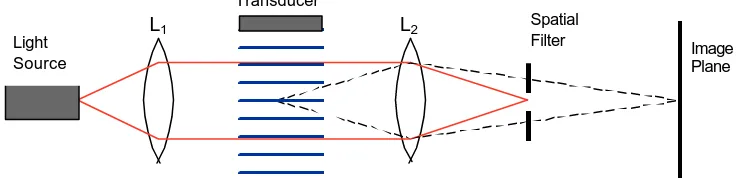
A slight change in the optical arrangement of Fig. 1 allows an optical image of the sound field to be ceated. The relevant technique stems from A. Toepler and dates back to the year 1866. Fig. 2 shows a typical experimental arrangement. By means of lens L2, the central plane of the

sound field is imaged on the image plane. To create an image, some spatial filtering is necessary. For dark field illumination, the central diffraction order is blocked and the higher orders pass the Schlieren stop. Contrary to this, bright field illumination is obtained if the central diffraction order passes the slit aperture and the higher orders are blocked (as shown in Fig. 2).

Fig. 2. Typical experimental arrangement for Schlieren imaging L2

L1

Image Plane Transducer

Light Source

Transducer

Diffraction Pattern

x

y

z

Light Source

2.3 Laser Interferometry

Another acousto-optical technique used for ultrasonic field investigations is based on laser interferometry [4]. Fig. 3 shows a typical set-up. The arrangement presented is that of a Michelson interferometer. The probing laser beam twice traverses the sound field. Due to the changes of the refractive index in the ultrasonic field, the optical phase is changed. Disregarding the factor two, the optical phase retardation is the same as for light diffraction (eq. (2)).

Fig. 3. Typical experimental arrangement for laser interferometry

3 SELECTED APPLICATIONS

3.1 High Speed Schlieren Imaging

When a continuous light source is used in the experimental arrangement shown in Fig. 2, a time-averaged Schlieren image is obtained. In this case, the optical image shows the spatial distribution of the sound pressure. Additionally, information on the phase surfaces is obtained using a pulsed light source whose pulse duration must be short compared with the time constant of the ultrasonic wave. Fig. 4 shows three situations of an ultrasonic tone burst before, during and after reflection off a cylindrically curved reflector.

Fig. 4. High speed Schlieren photograph of an ultrasonic wave reflected off a cylindrically curved reflector at different instants. Frequency: 0.5 MHz; medium: water

The images reveal that the Schlieren technique quickly gives a very useful overall impression of the sound field, which cannot be obtained from point-by-point measurements. For quantitative pressure information, additional measurements are to be carried out. It should be noted that the Schlieren technique always furnishes the projection of the sound field, which means that no details can be distinguished in the direction of light propagation.

Reference Mirror Photodiode

Object Mirror Laser

3.2 Field Mapping by Light-diffraction Tomography

The evaluation of the diffraction pattern mentioned in section 2.1, does not allow direct actual field mapping. If, however, the experimental set-up of Fig. 2 is used with the zero and one of the first diffraction orders passing the spatial filter, the normalized light intensity is obtained in the image plane [5]:

)) , ( cos( )) , ( ˆ ( )) , ( ˆ ( 2 )) , ( ˆ ( )) , ( ˆ ( ) , ,

( 0 1

2 1 2

0 v x z J v xz J v xz J v x z t Kz x z

J t z x

I = + ± Ω − +ϕ . (3)

The first two terms on the right side represent the dc component of the light intensity. The third term expresses the time modulation component caused by the interference of the zeroth diffraction order and the Doppler-shifted first diffraction order. From the point of view of quantitative sound field mapping, only the interference term is of interest. Eq. (3) can be further simplified for small sound pressure amplitudes:

)) , ( cos( ) , ( ˆ 1 ) , ,

(x zt v x z t Kz x z

I = ± Ω − +ϕ . (4)

In order to verify eqs. (3) and (4) experimentally, a high spatial resolution of the optical detection system is necessary. This can be achieved by magnified imaging of the sound field onto the image plane and by the use of a small aperture photodiode. From eq. (2) it is obvious that v is proportional to the mean value of the sound pressure over the width of the sound field. As a consequence, a tomographic evaluation needs to be carried out after data acquisition.

-10 0 10 20 -20 -10 0 10 20 0 10 20 30 40

Sound Pressure (kPa)

Y Axis (mm) X Axis (mm)

-20 -10 0 10 20 -20 -10 0 10 20 0,0 2,5 5,0 7,5 10,0 12,5 15,0 17,5

Sound Pressure (kPa)

Y Axis (mm)

X Axis (mm)

Fig. 5. Sound pressure distribution in the Fresnel zone of a circular (left) and of a square (right) transducer

Typical examples of the sound pressure distribution in a particular plane of the Fresnel zone for a circular and a square transducer are shown in Fig. 5. The circular transducer with a diameter of 20 mm is excited at a frequency of 2.25 MHz. The square transducer with a side length of 20 mm is excited at 3.33 MHz. The sound transmitting liquid is water (∂n/∂p=1.51×10−10Pa-1). Although the graphs are presented with a mesh width of only 1 mm×1 mm (sample interval 0.25 mm), the fine structure of the sound field can be clearly perceived.

Here, the discussion was limited to weak acousto-optical interaction, i.e. to the Raman-Nath regime. For further details of the limits of the Raman-Nath regime, sound field mapping under Bragg conditions and in the intermediate range between weak and strong acousto-optical interaction, the reader is referred to the literature [6,7].

3.3 Field Mapping by Laser Interferometry

) , , ( 2

1 1 ) , , (

R 0

t z x I I I k t z

x =

ξ , (5)

where I₀ and I_R are the light intensities in the object and the reference beam, respectively. This equation shows that the stabilized interferometer can directly measure the mean value of the time waveform of an ultrasonic pulse. Field mapping also requires tomographic evaluation.

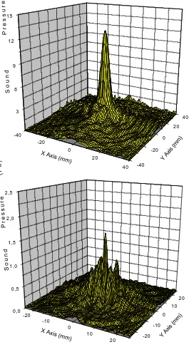
As an example, Fig. 6 shows pressure distributions of an electrostatic broadband speaker close to the surface of the source at 40 kHz and 120 kHz (∂n/∂p=2.7×10−9Pa-1). The flexible membrane of the speaker is assumed to have a diameter of about 15 mm. This diameter is about twice the wavelength in air at 40 kHz and about six times that at 120 kHz. As could be expected, the sound field is much more structured at 120 kHz than at 40 kHz. The maximum light-path change for 40 kHz is 324 pm and for 120 kHz it is 24 pm.

-40 -20

0

2 0

4 0 -40

-20 0

2 0 4 0 3

6 9 1 2 1 5

Sound Pressure (Pa)

Y Axis (mm)

X Axis (mm)

-20 -10

0 1 0

2 0 -20

-10 0

1 0 2 0

0,0 0,5 1,0 1,5 2,0 2,5

Sound Pressure (Pa)

Y Axis (mm) X Axis (mm)

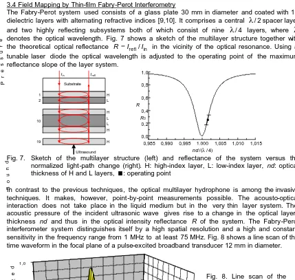
3.4 Field Mapping by Thin-film Fabry-Perot Interferometry

The Fabry-Perot system used consists of a glass plate 30 mm in diameter and coated with 19 dielectric layers with alternating refractive indices [9,10]. It comprises a central λ/2spacer layer and two highly reflecting subsystems both of which consist of nine λ/4 layers, where λ denotes the optical wavelength. Fig. 7 shows a sketch of the multilayer structure together with the theoretical optical reflectance R =Irefl/Iin in the vicinity of the optical resonance. Using a

tunable laser diode the optical wavelength is adjusted to the operating point of the maximum reflectance slope of the layer system.

R0

0,985 0,990 0,995 1,000 1,005 1,010 1,015

0,0 0,2 0,4 0,6 0,8 1,0

R

) 4 / /(λ nd

Fig. 7. Sketch of the multilayer structure (left) and reflectance of the system versus the normalized light-path change (right). H: high-index layer, L: low-index layer, nd: optical thickness of H and L layers, <: operating point

In contrast to the previous techniques, the optical multilayer hydrophone is among the invasive techniques. It makes, however, point-by-point measurements possible. The acousto-optical interaction does not take place in the liquid medium but in the very thin layer system. The acoustic pressure of the incident ultrasonic wave gives rise to a change in the optical layers thickness nd and thus in the optical intensity reflectance R of the system. The Fabry-Perot interferometer system distinguishes itself by a high spatial resolution and a high and constant sensitivity in the frequency range from 1 MHz to at least 75 MHz. Fig. 8 shows a line scan of the time waveform in the focal plane of a pulse-excited broadband transducer 12 mm in diameter.

0

1

2

3

4

0,0

0,2

0,4

0,6

0,8

1,0 -0,5

0,0 0,5 1,0

Normalized Sound Pressure

Time (µs) X Axis (mm)

REFERENCES

(1) P. Debye and F.W. Sears, Proc. Nat. Acad. Sci. (Washington) 18 (1932) 409 (2) R. Lucas and P. Biquard, J. Physique Radium 3 (1932) 464

(3) C.V. Raman and N.S.N.Nath, Proc. Indian Acad. Sci. (A) 2 (1935) 406 (4) O. Bou Matar et al., Proceedings 2000 IEEE Ultrasonics Symposium (5) R. Reibold and W. Molkenstruck, Acustica 56 (1984) 180

(6) P. Kwiek, W. Molkenstruck and R. Reibold, Ultrasonics 35 (1997) 499 (7) P. Kwiek, W. Molkenstruck and R. Reibold, Ultrasonics 36 (1998) 775

(8) R. Reibold and W. Molkenstruck, in: Ultrasonic exposimetry, Eds. M.C. Ziskin and P.A. Lewin, CRC Press 1993, ISBN 0-8493-6436-1

(9) V. Wilkens and Ch. Koch, Optics Letters 24 (1999) 1026

(10)V. Wilkens, Fortschritte der Akustik, DAGA 2002, to be published

Fig. 8. Line scan of the normalized pressure vs. time in the focal plane of the transducer

1 2

10

19

H

H

H

H L

L Substrate

Ultrasound L