THE BALASSA-SAMUELSON HYPOTHESIS AND
ELDERLY MIGRATION
Hernando Zuleta
Oscar Ávila
Mauricio Rodríguez
SERIE DO C UM ENTO S DE TRA BA JO
No . 5 9
Ene ro 2 0 0 9
The Balassa-Samuelson Hypothesis and Elderly Migration
Hernando Zuleta♣ - Oscar Ávila♦ - Mauricio Rodríguez♠
Abstract
We present an Overlapping Generations Model with two final goods: tradable goods are produced with a standard Cobb-Douglas production function and non-tradable goods are produced with linear production function where the only factor is labor. We maintain the fundamental assumption of factor mobility between sectors so model is consistent with the Balassa-Samuelson hypothesis. Given the general equilibrium structure of our model we can examine the effect of the saving rate on migration and non-tradable relative prices. Under this setting, we find that the elderly have incentives to migrate from economies where productivity is high to economies with low productivity because of the lower cost of living. In more general terms the elderly migration is likely to go from rich to poor countries. We also find that, for poor countries, the elderly migration has a positive effect in wages and capital accumulation.
Key words: tradable and non-tradable, overlapping generations, Balassa-Samuelson, elderly migration.
JEL classification: E21, E22, E23, E24, F21, F22, F43, J14, O41.
1. Introduction
The literature on international trade provides empirical evidence showing regularities regarding the relation between tradable and non-tradable prices and income level of the economies. Tradable prices tend to equalize among economies, due to the fact that those goods are subject of international trade. On the other hand, non-tradable goods’ prices may present significant differences between countries since international arbitrage is not possible. In particular, richer countries have higher non-tradable prices.1
This evidence is consistent with the Balassa-Samuelson (B-S) hypothesis which establishes that relative price of non-tradable grows when Total Factor Productivity (TFP) of the tradable sector increases relatively to TFP of the non-tradable2 sector. This result is based on the assumption of factor mobility between sectors: a raise in TFP of
♣ Visiting Professor, Economics Department, Brown University. Titular Professor (on leave), Facultad de
Economía, Universidad del Rosario.E-mail: hernando.zuleta84@urosario.edu.co
♦ Research Assistant, Facultad de Economía, Universidad del Rosario. E-mail: oscar.avila03@gmail.com ♠ Research Assistant, Facultad de Economía, Universidad del Rosario. E-mail: mand.rod@gmail.com
1 See De Gregorio, Giovannini and Wolf (1993); Falvey and Gemmel (1996); Ito, Isard and Symansky
(1997); Égert (2002) and Dobrinsky (2003) among others.
the tradable sector (ceteris paribus) generates a wage increase in that sector and, as a result, labor moves from the non-tradable sector to the tradable sector. Therefore, labor decreases in the non-tradable sector and the supply of non-tradable goods falls. Finally, the decrease in the supply of non-tradable goods and the increase in the supply of tradable goods generate an increase in the relative price of non-tradable goods.
A corollary of the B-S hypothesis is that if we assume purchasing power parity for tradable goods, when the TFP growth of the tradable sector is higher in country A relative to country B, the real exchange rate of country A must appreciate3.
Other branch of the literature, explain that workers try to move to high productivity locations because wages are positively correlated with productivity (see Sjaastad, 1962; Hicks, 1966 and Borjas, 1989, among others). Therefore, migrations reduce wage differentials between rich and poor countries and may help to reduce also the income gap. Now, the rationale for elderly migration is different. Old people do not work so they do not look for higher wages; on the contrary, they look for low prices and for this reason they are likely to migrate to low-wage countries.
Several authors have studied the phenomenon of elderly migration and, particularly, the cases of migration from the countries of North Europe to Center and South of the same continent, and from the Northern states of the U.S. to the Southern states and Mexico. The pioneers in this field - Lenzer (1965), Goldscheider (1966), and Lawton and Nehmow (1976) - argue that the elderly migrate looking for better living standards, related to housing, health services, and lower living costs. More recent studies confirm the results of Lenzer, Goldscheider and Lawton and Nehmow and identify other determinants for elderly migration like comfortable climate.4
We provide a general equilibrium model with an overlapping generations structure and two final goods: tradable goods are produced with a standard Cobb-Douglas and non-tradable goods are produced with linear production function where the only factor is labor. We maintain the fundamental assumption of factor mobility between sectors so
3 See Appendix 1.
4 This change in the subject of study has been motivated by the elderly migration growth during the last
the model is consistent with the B-S hypothesis. Under this setting, we find that the elderly have incentives to migrate from economies where productivity is high to economies with low productivity because of the lower cost of living. We also find that when countries differ in their saving rates, elderly migrate to economies with lower saving rates due to same reason (lower cost of living). In more general terms the elderly migration is likely to go from rich to poor countries. Finally, for poor countries, elderly migration has a positive effect in wages and capital accumulation.
The paper is organized in five sections, including the current introduction. In the second section we present both theoretical and empirical background about the behavior of TNT prices and its relation with TFP, as well as a literature review concerning to elderly migration. In section three, the OLG-TNT theoretical model is presented. This section is divided in three subsections, i) consumer’s problem; ii) firm’s problem; and iii) long run equilibrium. In section four we present our model predictions over elderly migration and capital accumulation, under different TFPs and saving rates. In section five, we conclude.
2. Background
2.1 TNT prices and TFP, theoretical and empirical background.
Harrod (1933) established that the relative prices of non-tradable tend to be higher in those countries with higher per capita income. Some years later Kravis, Heston and Summers (1982) test this hypothesis, finding that production of tradable goods in poor countries is characterized by low productivity levels. Additionally, they show that lower levels of productivity in this sector generate lower wages, and, as a consequence, the prices of services and non-tradable goods are lower in countries with lower incomes.
prices and real per capita income of several countries, this result is explained, partially, by productivity differences between economies. Ito, Isard and Symansky (1997) prove that the relation between real exchange rate and economic growth of the B-S hypothesis holds for Japan, South Korea, Taiwan, Hong Kong and Singapore, and that it is not significant for Thailand, Indonesia and Malaysia. Finally, Gibson and Malley (2007) examine the Greek case and obtained that some proportion of the variation on relative tradable prices is explained by changes in sector productivities.
Additionally, there are many studies that test the B-S hypothesis for Central and Eastern European countries, these studies have been motivated by the real exchange appreciation experimented by those countries during their transition to a market economy. For example, Égert (2002) studies six central European countries from 1991 to 2001, finding that the evolution of relative prices of non-tradable is positively related to the dynamics of relative productivity of tradable sector. Dobrinsky (2003) tests the B-S hypothesis for 13 candidate countries to join EU in 2004, observing the existence of a negative relation between changes on real exchange rate and relative productivity. Dumitru and Jianu (2008) studied the Romanian case and found that if non-tradable prices had not been regulated, the B-S effect would have been of 2.6% approximately, and not of 0.6% as it was before.
According to the results described in this section, the empirical evidence supports the B-S hypothesis; that is, the difference between tradable and non-tradable prices is explained partially by the difference in sector productivities; moreover, it is possible to say that richer countries have higher non-tradable prices.
2.2 Elderly migration.
Cebula, Hughes and McCormick (1981) find that real state costs affect the probability that individual migrate between regions within the UK. Cebula (1993) estimates that lower living costs have a significant impact on immigration, especially on elderly immigration. Rowles and Watkins (1993) study the effects of elderly migration over different receptor communities in the US. They present a theoretical model that describes the costs and benefits of migration. The main benefit of allowing immigration is that it can incentivize economic growth through the increase in the demand of goods and services, and the augment in the stock of capital. 5
In the same line, Watkins, y Pauer (1992), Severinghaus (1990), Fagan (1988), Gardner (1988), Rowles, Summers y Hirschl (1985), show that policymakers often consider elderly immigration as an important determinant for economic growth, so attracting elderly immigration can be considered as a development strategy.
Millington (2000) studied the determinants migration in the UK for three groups classified by age. He found that young people migrate from zones with lower raises in average wages and low growth in employment to zones with lower unemployment and faster growth in wages. While elderly are interested in lower rates of criminality and better weather, when decide where to migrate.
Elderly immigration seems to be desirable, thus it is necessary to determine the conditions that stimulate it. In this sense, Rowles and Watkins (1993) and Longino, et al. (2002), in their studies about elderly migration to Florida find warm climate, landscape, opportunity for leisure and entertainment, lower living costs and health and security services, as the main characteristics of an attractive destination for elderly migration.
The novelty of our paper is that it incorporates the B-S hypothesis into a general equilibrium model of economic growth, allowing us to analyze the effect of the hypothesis over consumption, migration and production decisions. It also relates two branches of the economic literature (B-S hypothesis and elderly migration), that until now seem to be separated, and it is consistent with the empirical evidence in both fields.
5 Similar results can befound in Fagan (1988), Happle, Hogan and Sullivan (1988), Longino and Crown
3. Overlapping Generations Model with Tradable and Non-tradable goods
The basic OLG model with production considers the existence of two generations of agents at any time, these agents live for two periods and individuals from all generations have the same preferences. During their lifetime they consume and get a positive utility of that. Agents work when they are young (first period of life) and get a wage equal to their productivity, part of this wage goes to consumption and the remaining is saved; then savings are devoted to build or buy capital. Finally, during the second period of life, agents are old and expend all their savings and its returns on consumption.
As described in the first section, in the model we present there is no long run growth. There are no externalities or exogenous technical change so the model is consistent with the conclusions of the neoclassical model of economic growth, Solow (1956) and Swan (1956), in which saving rate is the main determinant of the long run stock of physical capital (income).
We consider two final goods: tradable goods are produced with a standard Cobb-Douglas and non-tradable goods are produced with linear production function where the only factor is labor. The two final goods enter in the utility function in the standard way.
Finally, we make the usual simplifying assumptions of no population growth and physical capital depreciation equal to 1.
3.1 Consumers
Consumers’ objective is to maximize their utility, choosing present and future consumption of tradable and non-tradable goods during their first period of life. According to this and assuming an intertemporal logarithmic utility function, we have:
) ln (ln
ln
ln , , , 1 To,t 1
o t NT y
t T y
t
NT C C C
C
Where is the young agent consumption of non-tradable goods at time t; is the young agent consumption of tradable goods at time t; is the old agent
consumption of non-tradable goods at time t+1; is the old agent consumption of non-tradable goods at time t+1 and
y t NT
C , y
t T C , o t NT C ,+1 o
t T C ,+1
β is the discount factor. We use tradable goods as numéraire so,
1
; ,
,
, =
= Tt t T t NT t P P P P
Where is the relative price of non-tradable goods (in terms of tradables), considering price of tradables as numérarie. Therefore, we can write the budget constraint as follows: t P 1 1 , 1 , 1 , , 1 + + + + + + + + = t o t T o t NT t y t T y t NT t t r C C P C C P
w (BC)
Consumers maximize their utility subject to their budget constraint. From the first order conditions we have:
y t NT t y t
T PC
C , =γ , (2)
y t NT t t t o t
NT r C
P P
C 1 ,
1 1
, (1 + ) +
+ =β + (3)
y t NT t t o t
T P r C
C ,+1 =γβ (1+ +1) , (4)
(2), (3) and (4) in BC
) 1 )( 1 ( , = +γ +β t y t NT t w C
P (5)
Replacing (5) in (2), (3) y (4), we find:
) 1 )( 1 ( , γ β γ + + = t y t T w
C (6)
) 1 )( 1 ( ) 1 ( 1 1 ,
1 γ β
β + + + = + +
+ oNTt t t
t
r w C
P (7)
) 1 )( 1 ( ) 1 ( 1 1 , γ β γβ + + + = +
+ t t
o t T
r w
Given the preferences described above we observe that tradable and non-tradable consumption is directly proportional to labor income, and inversely proportional to the own price. It is also evident that old people’s consumption depends positively on the interest rate too, since it determines saving returns.
Saving on this economy is determined by the difference between young’s income and their tradable and non-tradable consumption. According to this, saving is:
⎟⎟ ⎠ ⎞ ⎜⎜ ⎝ ⎛ + = ⎟⎟ ⎠ ⎞ ⎜⎜ ⎝ ⎛ + + + = − − = β β β γ γ β 1 ) 1 )( 1 ( ) 1 ( ,
, t t
y t T y t NT t t
t w PC C w w
S (9)
Physical capital is the only accumulative factor in this economy, for this reason total saving at t must be equal to the stock of physical capital at t+1, this result comes from the total capital depreciation from t to t+1 assumption, in other words δ =1. As a consequence:
t
S =Kt+1 (10)
From (9) we can observe a positive relation between the discount factorβ, and total
savings. This result is obvious since people that have a higher valuation for the future consumption decide to save a larger amount of their resources.
3.2Firms
•Tradable Sector.
t T t t t t T t t
T AK L rK wL ,
1 ,
, = − −
Π α −α (11)
From the first order conditions we have:
α α α − − = 1 , 1 t T t
t AK L
α α
α −
−
= t Tt
t AK L
w (1 ) . (13)
•Non-tradable Sector.
t NT t t NT t t
NT, =BPL , −w L ,
Π (14)
From the first order conditions we have:
t
t w
BP = (15)
Free mobility of factors between sectors assumption allows the existence of a unique equilibrium wage on this economy; therefore, this assumption implies that equations (13) and (15) can be equalized. From this condition we find price’s dynamics during the transition, that is:
B L AK
P t Tt
t
α α
α −
−
=(1 ) . (16)
This equation establishes that non-tradable relative prices in the short run depend positively on physical capital per worker on the tradable sector. Condition (16) also says that economies with higher stock of physical capital, ceteris paribus, have higher non-tradable prices, at least in the short run. In addition, equation (16) is consistent with the B-S hypothesis, since an increase on TFP on tradable sector relative to TFP on non-tradable sector (i.e. a growth in A/B) ceteris paribus, increases non-tradable relative prices.
3.3 Equilibrium.
Having relative prices as a function of physical capital, and physical capital as a function of the number of workers on tradable sector, we must determine the number of workers in each sector in order to characterize the steady state.
t o t T o t NT P C C γ 1 ,
, = (2)’
Aggregating consumption using (2) and (2)’ we have:
t t T t NT P C C γ 1 ,
, = For all t (17)
Knowing that non-tradable consumption must equalize non-tradable production and tradable consumption must be equal to production less savings, we find:
( ) α α α β β α ⎟⎟ ⎠ ⎞ ⎜ ⎜ ⎝ ⎛ ⎟⎟ ⎠ ⎞ ⎜⎜ ⎝ ⎛ + − − = = − t T t t T t t T t NT t NT L K A L AK C BL C , 1 , , , , 1 1 (18)
We consider labor force as a constant, i.e. . Therefore, from (16), (17) and (18) it follows that
__ ,
, L L
LNt+ NTt =
(
)
__ __ , 1 1 ) 1 ( 1 1 L LLNTt ⎟⎟≤
⎠ ⎞ ⎜⎜ ⎝ ⎛ + − − − + = β β α α
γ (19)
and ⎟⎟ ⎠ ⎞ ⎜⎜ ⎝ ⎛ + − + − + − + − = ) 1 )( ) 1 ( 1 ( ) 1 ( ) 1 ( 1 ) 1 ( __ β γ α β α γ α γ α L
LT (20)
Equations (19) and 20 show that the number of workers in each sector is constant during the transition to the steady state; consequently, physical capital in t+1 depends only on the economy’s parameters and the stock of capital in t.
Note that 0 ; 0 ; 0 ) 1 ( ;
0 __ >
∂ ∂ < ∂ ∂ < − ∂ ∂ < ∂ ∂ L L L L
LNT NT NT NT
β α
γ and
0 ; 0 ; 0 ) 1 ( ;
0 __ >
∂ ∂ > ∂ ∂ > − ∂ ∂ > ∂ ∂ L L L L
LT T T T
β α
γ
Therefore, the number of workers in the non-tradable sector depends inversely on: i) tradable consumption importance on the utility function (consumer’s preferences); ii) labor share on tradable production function; and iii) the discount rate.
The first relation is a result of consumer’s preferences, since a higher preference for tradable goods and services implies a higher allocation of resources on this sector, reducing availability of labor for the non-tradable sector. On the other hand, the more labor intensive tradable sector is the more resources this sector gets. Finally, the last relation comes from the fact that saving is positively related to the discount rate and knowing that physical capital is the only cumulative factor, a higher discount rate implies a higher stock of physical capital, which increases labor productivity in the tradable sector, so the number of workers on this sector increase, due to the free labor mobility.
3.4 Long Run Equilibrium.
In order to characterize economy transition to the steady state we use equations (9), (9’) and (12), getting the physical capital transition equation (TE):
α α
α β
β −
+ ⎟⎟ −
⎠ ⎞ ⎜⎜ ⎝ ⎛
+
= t Tt
t AK L
K 1 (1 ) ,
1 (TE)
Using steady state definition (i.e. variables do not change in time, t=t+1=ss) we have:
α α
β β
α − −
⎟⎟ ⎠ ⎞ ⎜⎜
⎝ ⎛
⎟⎟ ⎠ ⎞ ⎜⎜ ⎝ ⎛
+ −
= 1
1
1 )
1
( Tss
ss AL
K (21)
Replacing (15) in (9):
⎟⎟ ⎠ ⎞ ⎜⎜ ⎝ ⎛
+ =
β β
1
ss
ss BP
Equations (21) and (22) show that steady state capital stock capital depends inversely on the number of workers on tradable sector, and directly on the marginal productivity of workers on non-tradable sector. This result comes from the fact that workers marginal productivity in the non-tradable sector is constant, and this productivity determines labor remuneration in the whole economy. In this way, a higher B reduces the number of workers in the tradable sector, increasing labor productivity in this sector, and then equalizing wages in both sectors; this result implies that a higher B increases wages and considering the positive relation between income and savings, the latter increases and so does the physical capital. On the other hand, from equation (17) we observe that relative prices are positively related with the stock of physical capital of the economy.
Combining with equations (20) and (21)
α α β β β γ α β γ α γ α − − ⎟ ⎟ ⎟ ⎠ ⎞ ⎜ ⎜ ⎜ ⎝ ⎛ ⎟⎟ ⎠ ⎞ ⎜⎜ ⎝ ⎛ + ⎥ ⎥ ⎦ ⎤ ⎢ ⎢ ⎣ ⎡ ⎟⎟ ⎠ ⎞ ⎜⎜ ⎝ ⎛ + − + + − + − = 1 1 __ 1 ) 1 )( ) 1 ( 1 ( ) 1 ( 1 ) 1
( A L
Kss (23)
Getting back to equation (16), that shows price’s dynamics to the steady state, we observe that relative prices of non-tradables in terms of tradables only changes when the physical capital does, because the number of workers is fixed in each moment of time. This relation shows that countries with a higher initial stock of physical capital have higher non-tradable relative prices during the transition, if they do not differ in anything else.
4. Capital flows and elderly migration
In this section we present three scenarios that allow us to establish the conditions under which capital flow and elderly migration between countries would occur. We first consider the case of two economies identical in all but the amount of capital. Then we consider two economies with different TFP level. Finally, we consider two economies with different saving rates.
Consider two hypothetical economies, which differ only on their initial stock of physical capital. The economy that starts with the lower stock of physical capital has cheaper non-tradable goods and services during the transition to the steady state (see equation (16)). Nonetheless, in the long-run equilibrium prices and capital of both countries will converge.
Similarly, if we consider two identical economies in all but the amount of workers, the more labor abundant economy (as the developing economies), has lower non-tradable relative prices, even in the long run equilibrium. By simulating the transition of two economies which only differ on the number of workers we find that the more labor abundant has lower non-tradable relative prices, not only during the transition to the steady state, but also on the long run equilibrium (see Appendix 3, Figure 5).
These results are consistent with the conclusions made by Harrod (1933) and Kravis, et al. (1982).
In both cases, the elderly have incentives to migrate from the capital abundant country to the labor abundant country. Now, if the elderly migration is large enough, it generates an equalization of non tradable prices and, for this reason, wages immediately converge to the same level. Therefore, after one period the stock of capital and the income per worker of the two economies converge to the same level.
4.2 The Balassa-Samuelson effect (differences in TFP)
Considering two economies that are identical except for the TFP in both sectors (parameters A and B), from the steady state equations of price and capital we have:
Let and be country i’s TFPs in tradable and non-tradable sector respectively, with and , we have:
i A Bi
j
i A
A ≠ Bi ≠Bj
α
−
⎟ ⎟ ⎠ ⎞ ⎜ ⎜ ⎝ ⎛
= 1
1
j i
ssj ssi
A A K
K
⎟⎟ ⎠ ⎞ ⎜⎜ ⎝ ⎛ ⎟ ⎟ ⎠ ⎞ ⎜ ⎜ ⎝ ⎛
= −
i j
j i
ssj ssi
B B A
A P
P 1α
1
(25)
Under this scenario the gap in steady state’s capital only depends on the relation of the tradable sectors TFPs, thus countries with a higher TFP in the tradable sector will have a higher level of income in the long run (considering the stock of capital as a proxy of the level of income). Moreover, i’s non-tradable relative prices will be higher if:
( )
−α( )
−α> 1
1 1
1
j j
j i
B A B
A
(25’)
Condition (25’) implies that elderly will have incentives to migrate from country i to country j, due to the lower living costs of j. Under the B-S hypothesis implications over the Real Exchange Rate (RER), (25’) also establishes that country i’s currency will appreciate in real terms against j’s currency during the transition to the steady state. Nonetheless, if i and j only differ in their TFPs interest rates in the long run will be the same in both economies (see equation (11)), so there will not be capital flow between countries.
Then if and (25’) hold, i will be richer in the long run and elderly will have incentives to migrate from i to j, since j have lower living costs. Nevertheless, this migration will not be accompanied by a capital flow in neither direction.
j
i A
A >
If elderly migrate from one country to another we have that non-tradable consumption is modified in both countries.
As non-tradable production only uses labor, this one must flow between sectors in order to satisfy condition (18). Defining ψ as 1 plus the growth rate of non-tradable consumption due to the elderly migration, and using (16), (17) and (18) we have:
t NT t
NT BL
C , = ,
Thus, the new non-tradable labor is:
(
)
____
, 1
1 ) 1
( L L
LNTt ⎟⎟≤
⎠ ⎞ ⎜⎜
⎝ ⎛
+ − − − + =
β β α α
γ ψ
ψ
From this expression we can derive that:
0 ;
0 ;
0 ;
0 , __
, >
∂ ∂ > ∂ ∂ < ∂ ∂ > ∂ ∂
ψ ψ
ψ
ψ t t
t T t
NT L K P
L
Intuitively, from condition (18) we know that non-tradable production must be equal to its consumption, and due to elderly migration we have that non-tradable consumption diminishes (increases) in the origin (receptor) country.
In the country with higher TFP (origin country) labor flows from non-tradable sector to tradable sector; then, tradable production increases. Elderly migration also pushes non-tradable prices down. From equation (16) we have that more workers on non-tradable sector affect negatively non-tradable prices and reduce wages, since labor productivity decreases. As we can see, labor mobility allows the economy to reach a new equilibrium with a lower level of capital and non-tradable prices.
In the country with lower TFP (receptor country) we have the opposite effects: aggregate consumption, wages, non-tradable production and prices rise. We can also identify a positive effect of elderly migration for this country, since labor mobility from tradable to non-tradable sector increases wages and the stock of capital.
4.3 Different saving rates
Economies around the world have different dispositions to save; even economies with a similar degree of development can have dissimilar saving rates (i.e. U.S. and Japan). Next we consider two economies with different discount factors (β), thus with different
saving rates (
(
)
β β σ
+ =
Let βi be the discount factor for country i, withβi ≠βj, we can observe the relation between the saving rate and the stock of capital, the relative prices, and the interest rate, in the steady state.
From (20) and (21):
( )
(
(
)
)
(
(
)
)
⎥ ⎦ ⎤ ⎢ ⎣ ⎡ ⎟⎟ ⎠ ⎞ ⎜⎜ ⎝ ⎛ − + − − ⎟⎟ ⎠ ⎞ ⎜⎜ ⎝ ⎛ = ⎥ ⎦ ⎤ ⎢ ⎣ ⎡ + − + − − = ∂ ∂ − − − Tss Tss ss Tss Tss ss ss L L K A L L K A K σ α γ α α σ α γ α α σ α α α α 1 1 1 1 1 1 1 1 (26) From (26): 0 > ∂ ∂ σss Kif
(
(
)
)
σα γ α α − + − > 1 1 1 Tss
L . From (20) we have that these condition always holds.
Then we have the basic outcome of the neoclassical growth theory, a country with a higher saving rate ceteris paribus, will we in richer in the long run.
About the effect of saving rate on non-tradable relative prices, from (22):
σ σ σ ∂ ∂ = − ∂ ∂ ss ss
ss BP B P
K
(27)
Thus, to know the sign of σ ∂ ∂Pss
, is necessary to know if Kss >BPss ∂
∂
σ holds or not.
From (16) and (26) 6, we find that σ ∂ ∂Pss >0.
Equations (26) and (27) imply that countries with a higher saving rate σ will have a larger stock of capital and higher non-tradable prices in long run. Under this
See Appendix 3.
configuration of parameters the elderly will be incentivize to migrate to countries with lower saving rates, because of the lower living costs7.
To characterize the effect of saving rate on steady state’s interest rate, from (12) we have: α α α − − = 1 , 1 ss T ss
ss AK L
r
By observing this equation is possible to identify two opposed effects of the saving rate on the interest rate. A higher saving rate cause an increase in the stock of capital, reducing capital’s productivity, then reducing the interest rate. On the other hand, a higher saving rate increases the labor proportion in the tradable sector, increasing capital’s productivity, and then increasing the interest rate.
Deriving by the saving rate:
(
)
⎥ ⎦ ⎤ ⎢ ⎣ ⎡ ⎟ ⎠ ⎞ ⎜ ⎝ ⎛ ∂ ∂ − ⎟⎟ ⎠ ⎞ ⎜⎜ ⎝ ⎛ ∂ ∂ − = ∂ ∂ − − σ σ α α σ α α ss Tss Tss ss Tss ss ss K L L K L K A r 2 1 (28)Though the determination of the sign in (28) is not immediate, focusing on the expression: ⎥ ⎦ ⎤ ⎢ ⎣ ⎡ ⎟ ⎠ ⎞ ⎜ ⎝ ⎛ ∂ ∂ − ⎟⎟ ⎠ ⎞ ⎜⎜ ⎝ ⎛ ∂ ∂ σ
σ Tss ss
Tss ss K L L K , Solving σ ∂
∂Kss and reorganizing the expression:
[
α ασ]
α σ − − − + − ∂∂ 1 1
Tss Tss
ss
Tss K AL AL
L
7For a simulation of two hypothetical economies with different saving rates, see Appendix 3. Figure 7 and
From this last expression is possible to observe that increases in the tradable sector’s
labor, generate a decrease in σ ∂
∂rss , specifically:
∞ = ∂ ∂
→ σ
ss L
r
Tss 0
lim And =−∞
∂ ∂
∞
→ σ
ss L
r
Tss
lim
Intuitively, this result implies that economies with a lower quantity of workers in the tradable sector (as in the developing economies) will experience positive effects of the saving rate on the interest rate. This is due to the fact that with a low participation of
labor in the tradable sector the positive effect that has the increase in overcomes the
negative effect of the increase in the stock of capital.
Tss
L
Under this assumption we have two sceneries: elderly migrate without their capital, and elderly migrate with capital. The first scenario generates the same results as described on section 4.1. Under the second scenario, the direction of the effects is the same but the magnitude increases, in other words, the effects are reinforced.
5. Concluding remarks
The model developed in this document is consistent with the B-S hypothesis referent to the non-tradable relative prices and real exchange rate dynamics, since it maintains the fundamental assumption of free mobility between sectors. It establishes that not only relative prices but also the real exchange rate depends on the relative TFP between sectors.
On the same way, this model allows us to explain the effect of TFP on elderly migration. In particular, we find that economies with a higher relative TFP have higher living costs, given the B-S hypothesis and under PPP, since non-tradable goods and services are more expensive, according to the empirical evidence old people would migrate to countries with lower TFP (cheaper non-tradable goods and services).
increases tradable production, while for the receiving country it has the opposite effects, and increases the stock of capital.
Elderly migration benefits the receptor country either if old people migrate with their physical capital or not. If they migrate with their capital is obvious why the receptor economy benefits, since this factor stimulates economic activity and increases economic growth. If they do not migrate with their capital, migration still has a positive effect due to the increase in wages, then in saving and in the economic growth.
References
1. Balassa, B. (1964). The Purchasing-Power Parity Doctrine: A Reappraisal. The Journal of Political Economy, 72 (6), 584-596.
2. Borjas, G. (1989). Economic Theory and International Migration. International Migration Review, 23 (3), 457-485.
3. Cebula, R. (1993). The Impact of Living Costs on Geographic Migration. The Quarterly Review of Economics and Finance, 33 (1), 101-105.
4. Dobrinsky, R. (2003). Convergence in Per Capita Income Levels, Productivity Dynamics and Real Exchange Rates in the EU Acceding Countries. Empirica, 30, 305-334.
5. Dumitru, I., & Jianu, I. (2008). The Balassa-Samuelson effect in Romania - The role of regulated prices. European Journal of Operational Research , doi:10.1016/j.ejor.2007.12.026.
6. Égert, B. (2002). Investigating the Balassa-Samuelson hypothesis in transition: Do we understand what we see? BOFIT Discussion Papers (6).
7. Fagan, M. (1988). Attracting Retirees for Economic Development. Jacksonville, AL: Center for the Economic Development and Business Research, Jacksonville State University.
8. Falvey, R., & Gemmel, N. (1996). A Formalization and Test of the Factor Productivity Explanation of International Differences in Service Prices.
International Economic Revie, 37 (1), 85-102.
9. Froot, K., & Rogoff, K. (1994). Perspectives on PPP and Long-Run real exchange rate. National Bureau of Economic Research (Working Paper 4952). 10.Gardner, R. (1988). Attracting retirees to Idaho. A rural development strategy.
Idaho Economic Forecast, 9 (3), 28-46.
11.Gibson, H., & Malley, J. (2007). The Contribution of Sectoral Productivity Differentials to Inflation in Greece. Open Economies Review .
12.Goldscheider, C. (1966). Differencial Residential Mobility of the Older Population. Journal of Gerontology, 21, 103-108.
13.Happel, S., Hogan, T., & Sullivan, D. (1988). Going away to roost. American Demographics, 6 (6), 33-45.
15.Hodge, G. (1991). The economic impacts of retirees on smaller communities.
Research on Aging, 13 (1), 39-54.
16.Hughes, G., & McCormick, B. (1981). Do Council Housing Policies Reduce Migration Between Regions? The Economic Journal, 91 (364), 919-937.
17.Illés, S. (2005). Elderly Immigration to Hungary. Migration Letters, 2 (2), 164-169.
18.Ito, T., Isard, P., & Symansky, S. (1997). Economic Growth and Real Exchange Rate: An Overview of the Balassa-Samuelson Hypothesis in Asia. National Bureau of Economic Research (Working Paper 5979).
19.Kravis, I., Heston, A., & Summers, R. (1982). The Share of Services in Economic Growth. En F. Adams, & B. Hickman (Edits.), Global Econometrics: Essays in Honor of Lawrence R. Klein. Cambridge: MIT Press.
20.Lawton, M., & Nahemow, L. (1976). Ecology in the Aging Process. (A. P. Association, Ed.) Washington D.C.: C. Eisdorfer y M.P. Lawton.
21.Lenzer, A. (1965). Mobility Patterns Among the Aged. Gerontologist, 5 (1), 12-15.
22.Longino, C., Perzynski, A., & Stolle, E. (2002). Pandora’s Briefcase: Unpacking the Retirement Migration Decision. Research on Aging , 24-29.
23.Longino, C., & Crown, W. (1989). The migration of old money. American Demographics , 28-31.
24.Millington, J. (2000). Migration and Age: The Effect of Age on Sensivity to Migration Stimuli. Regional Studies, 34 (6), 521-533.
25.Rowles, G., & Watkins, J. (1993). Elderly Migration and Development in Small Communities. Growth and Change, 24, 509-538.
26.Rowles, G., Watkins, J., & Pauer, G. (1992). Impact of Migration of the Elderly.
Lexington, KY, Sanders - Brown Center on Aging, Final Report to the Appalachian Repional Commission, Contract No. 90 - 4, CO - 10257 - 89 - I - 302 - 0321 .
27.Samuelson, P. (1964). Theoretical notes on trade problems. The Review of Economics and Statistics, 46, 145-154.
29.Sjaastad, L. (1962). The Costs and Returns of Human Migration. The Journal of Political Economy, 70 (5), 80-93.
30.Solow, R. 1956. “A Contribution to the Theory of Economic Growth” The Quarterly Journal of Economics 70(1): 65-94.
31.Summers, G., & Hirschl, T. (1985). Retirees as a growth industry. Rural Development Perspective, 1 (2) , 13-16. Rockville, MD: U.S. Department of Agriculture.
32.Swan, Trevor W. (1956) “Economic Growth and Capital Accumulation.”
Appendix 1
P EP
q= *
Where:
q: Is the Real Exchange Rate. E: Is the Nominal Exchange Rate. P: Is the Domestic Price Index. P*: Is the Foreign Price Index.
Constructing price indexes and assuming that participation of tradable and non-tradable are the same in both countries, we have:
( ) (
γ)
−γ= 1
NT
T P
P P
( ) (
γ)
−γ= 1
* *
* PT PNT P
Assuming PPP for tradable goods and services, we have:
(
) (
)
( ) ( )
γ
γ γ
γ
γ −
− −
⎟⎟ ⎠ ⎞ ⎜⎜
⎝ ⎛ = =
=
1
1 1
* *
* *
NT NT
NT T
NT T
P P P
P P P E P EP q
Appendix 2
Thus, to know the sign of σ ∂
∂Pss . From (16) and (26) we just need to compare:
(
)
(
)
⎟⎟⎠ ⎞ ⎜⎜ ⎝ ⎛ − +
− −
Tss L
σ α γ
α α
1 1
1
1 Vs
(
1−α
)
equivalent to:(
)
(
)
⎟⎟⎠ ⎞ ⎜⎜ ⎝ ⎛ − +
−
Tss L
σ α γ
α α
1 1
1
Vs
α
, from (22) we have:(
)
(
1)
11 1
< ⎟⎟ ⎠ ⎞ ⎜⎜ ⎝ ⎛ − +
−
Tss L
σ α γ
α
, so ss
ss BP
K
> ∂ ∂
Appendix 3
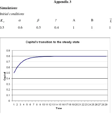
Simulations
Initial conditions o
K α β γ A B L
[image:26.595.86.465.72.461.2]0.5 0.6 0.5 0.4 1 1 1
[image:26.595.85.461.445.731.2]Figure 1. Source: Authors calculations.
Different levels of physical capital
α β γ A B L
[image:27.595.85.465.95.445.2]0.6 0.5 0.4 1 1 1
Figure 3. Source: Authors calculations.
[image:27.595.84.461.469.735.2]Different levels of labor force o
K α β γ A B
[image:28.595.85.463.75.427.2]0.5 0.6 0.5 0.4 1 1
Figure 5. Source: Authors calculations.
The Balassa-Samuelson Effect (different relative productivities) o
K α β γ B L
Figure 6. Source: Authors calculations.
Positive shock on the saving rate o
K α γ A B L
0.5 0.6 0.4 1 1 1
[image:29.595.85.461.172.747.2]