Lecture Notes in Financial Economics
c
by Antonio Mele
London School of Economics & Political Science
Preface . . . 13
I
Foundations
14
1 The classic capital asset pricing model 15 1.1 Portfolio selection . . . 151.1.1 The wealth constraint . . . 15
1.1.2 Portfolio choice . . . 16
1.1.3 Without the safe asset . . . 17
1.1.4 The market portfolio . . . 19
1.2 The CAPM . . . 21
1.3 The APT . . . 23
1.3.1 A first derivation . . . 23
1.3.2 The APT with idiosyncratic risk and a large number of assets . . . 25
1.3.3 Empirical evidence . . . 26
1.4 Appendix 1: Some analytical details for portfolio choice . . . 27
1.4.1 The primal program . . . 27
1.4.2 The dual program . . . 28
1.5 Appendix 2: The market portfolio . . . 30
1.5.1 The tangent portfolio is the market portfolio . . . 30
1.5.2 Tangency condition . . . 30
1.6 Appendix 3: An alternative derivation of the SML . . . 32
1.7 Appendix 4: Broader definitions of risk - Rothschild and Stiglitz theory . . . 33
References . . . 35
2.2 The static general equilibrium in a nutshell . . . 36
2.2.1 Walras’ Law . . . 37
2.2.2 Competitive equilibrium . . . 37
2.2.3 Optimality . . . 38
2.3 Time and uncertainty . . . 42
2.4 Financial assets . . . 43
2.5 Absence of arbitrage . . . 43
2.5.1 How to price a financial asset? . . . 43
2.5.2 The Land of Cockaigne . . . 45
2.6 Equivalent martingales and equilibrium . . . 49
2.6.1 The rational expectations assumption . . . 49
2.6.2 Stochastic discount factors . . . 50
2.6.3 Optimality and equilibrium . . . 51
2.7 Consumption-CAPM . . . 55
2.7.1 The risk premium . . . 55
2.7.2 The beta relation . . . 56
2.7.3 CCAPM & CAPM . . . 56
2.8 Infinite horizon . . . 56
2.9 Further topics on incomplete markets . . . 57
2.9.1 Nominal assets and real indeterminacy of the equilibrium . . . 57
2.9.2 Nonneutrality of money . . . 58
2.10 Appendix 1 . . . 59
2.11 Appendix 2: Proofs of selected results . . . 60
2.12 Appendix 3: The multicommodity case . . . 63
References . . . 65
3 Infinite horizon economies 66 3.1 Introduction . . . 66
3.2 Consumption-based asset evaluation . . . 66
3.2.1 Recursive plans: introduction . . . 66
3.2.2 The marginalist argument . . . 67
3.2.3 Intertemporal elasticity of substitution . . . 68
3.2.4 Lucas’ model . . . 69
3.2.5 Arrow-Debreu state prices, the CCAPM and the CAPM . . . 71
3.3 Production: foundational issues . . . 72
3.3.1 Decentralized economy . . . 72
3.3.2 Centralized economy . . . 73
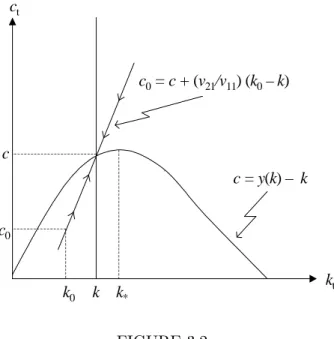
3.3.3 Dynamics . . . 74
3.3.4 Stochastic economies . . . 76
3.4 Production-based asset pricing . . . 80
3.4.1 Firms . . . 80
3.4.2 Consumers . . . 84
3.5 Money, production, asset prices, and overlapping generations models . . . 85
3.5.1 Introduction: endowment economies . . . 85
3.5.2 Diamond’s model . . . 88
3.5.3 Money . . . 88
3.5.4 Money in a model with real shocks . . . 92
3.6 Optimality . . . 93
3.6.1 Models with productive capital . . . 93
3.6.2 Models with money . . . 94
3.7 Appendix 1: Finite difference equations, with economic applications . . . 95
3.8 Appendix 2: Neoclassic growth in continuous-time . . . 99
3.8.1 Convergence from discrete-time . . . 99
3.8.2 The model . . . 100
3.9 Appendix 3: Control . . . 102
References . . . 103
4 Continuous time models 104 4.1 Lambdas and betas in continuous time . . . 104
4.1.1 The pricing equation . . . 104
4.1.2 Expected returns . . . 105
4.1.3 Expected returns and risk-adjusted discount rates . . . 105
4.2 An introduction to continuous time methods in finance . . . 106
4.2.1 Partial differential equations and Feynman-Kac probabilistic representa-tions of the solution . . . 106
4.2.2 The Girsanov theorem with applications to finance . . . 110
4.3 An introduction to no-arbitrage and equilibrium . . . 112
4.3.1 Self-financed strategies . . . 112
4.3.2 No-arbitrage in Lucas tree . . . 113
4.3.3 Equilibrium with CRRA . . . 114
4.3.4 Bubbles . . . 116
4.3.5 Reflecting barriers and absence of arbitrage . . . 117
4.4 Martingales and arbitrage in a diffusion model . . . 118
4.4.1 The information framework . . . 118
4.4.2 Viability . . . 119
4.4.3 Market completeness . . . 121
4.5 Equilibrium with a representative agent . . . 122
4.5.1 Consumption and portfolio choices: martingale approaches . . . 122
4.5.2 The older, Merton’s approach: dynamic programming . . . 125
4.5.3 Equilibrium . . . 126
4.5.4 Continuous-time Consumption-CAPM . . . 127
4.6 Market imperfections and portfolio choice . . . 128
4.7 Jumps . . . 129
4.7.1 Poisson jumps . . . 129
4.7.3 Properties and related distributions . . . 131
4.7.4 Some asset pricing implications . . . 132
4.7.5 An option pricing formula . . . 133
4.8 Continuous-time Markov chains . . . 133
4.9 Appendix 1: Self-financed strategies . . . 134
4.10 Appendix 2: An introduction to stochastic calculus for finance . . . 135
4.10.1 Stochastic integrals . . . 135
4.10.2 Stochastic differential equations . . . 144
4.11 Appendix 3: Proof of selected results . . . 150
4.11.1 Proof of Theorem 4.2 . . . 150
4.11.2 Proof of Eq. (4.48). . . 150
4.11.3 Walras’s consistency tests . . . 151
4.12 Appendix 4: The Green’s function . . . 152
4.12.1 Setup . . . 152
4.12.2 The PDE connection . . . 153
4.13 Appendix 5: Portfolio constraints . . . 154
4.14 Appendix 6: Models with final consumption only . . . 156
4.15 Appendix 7: Further topics on jumps . . . 158
4.15.1 The Radon-Nikodym derivative . . . 158
4.15.2 Arbitrage restrictions . . . 159
4.15.3 State price density: introduction . . . 159
4.15.4 State price density: general case . . . 160
References . . . 162
5 Taking models to data 163 5.1 Introduction . . . 163
5.2 Data generating processes . . . 163
5.2.1 Basics . . . 163
5.2.2 Restrictions on the DGP . . . 164
5.2.3 Parameter estimators . . . 165
5.2.4 Basic properties of density functions . . . 165
5.2.5 The Cramer-Rao lower bound . . . 166
5.3 Maximum likelihood estimation . . . 166
5.3.1 Basics . . . 166
5.3.2 Factorizations . . . 166
5.3.3 Asymptotic properties . . . 167
5.4 M-estimators . . . 169
5.5 Pseudo, or quasi, maximum likelihood . . . 170
5.6 GMM . . . 171
5.7 Simulation-based estimators . . . 174
5.7.1 Three simulation-based estimators . . . 175
5.7.2 Asymptotic normality . . . 177
5.7.4 Advances . . . 181
5.7.5 In practice? Latent factors and identification . . . 181
5.8 Asset pricing, prediction functions, and statistical inference . . . 182
5.9 Appendix 1: Proof of selected results . . . 186
5.10 Appendix 2: Collected notions and results . . . 187
5.11 Appendix 3: Theory for maximum likelihood estimation . . . 190
5.12 Appendix 4: Dependent processes . . . 191
5.12.1 Weak dependence . . . 191
5.12.2 The central limit theorem for martingale differences . . . 191
5.12.3 Applications to maximum likelihood . . . 191
5.13 Appendix 5: Proof of Theorem 5.4 . . . 193
References . . . 194
II
Asset pricing and reality
197
6 On kernels and puzzles 198 6.1 A single factor model . . . 1986.1.1 The model . . . 198
6.1.2 Extensions . . . 201
6.2 The equity premium puzzle . . . 201
6.3 Hansen-Jagannathan cup . . . 203
6.4 Multifactor extensions . . . 204
6.4.1 Exponential affine pricing kernels . . . 204
6.4.2 Lognormal returns . . . 206
6.5 Pricing kernels and Sharpe ratios . . . 207
6.5.1 Market portfolios and pricing kernels . . . 207
6.5.2 Pricing kernel bounds . . . 209
6.6 Conditioning bounds . . . 211
6.7 Appendix . . . 212
References . . . 215
7 The stock market 216 7.1 Introduction . . . 216
7.2 The empirical evidence: bird’s eye view . . . 216
7.3 Volatility: a business cycle perspective . . . 222
7.3.1 Volatility cycles . . . 223
7.3.2 Understanding the empirical evidence . . . 224
7.3.3 What to do with stock market volatility? . . . 229
7.3.4 What did we learn? . . . 234
7.4 Rational stock market fluctuations . . . 235
7.4.1 A decomposition . . . 235
7.4.3 Volatility, options and convexity . . . 237
7.5 Time-varying discount rates or uncertain growth? . . . 241
7.5.1 Markov pricing kernels . . . 242
7.5.2 External habit formation . . . 243
7.5.3 Large price swings as a learning induced phenomenon . . . 246
7.6 The cross section of stock returns and volatilities . . . 250
7.6.1 Returns . . . 250
7.6.2 Volatilities . . . 252
7.7 Appendix 1: Calibration of the tree in Section 7.3 . . . 253
7.8 Appendix 2: Arrow-Debreu PDEs . . . 255
7.9 Appendix 3: The maximum principle . . . 256
7.10 Appendix 4: Proofs of selected results . . . 258
7.11 Appendix 5: Bond price convexity revisited . . . 260
7.12 Appendix 6: Simulation of discrete-time pricing models . . . 261
References . . . 262
8 Tackling the puzzles 266 8.1 Non-expected utility . . . 266
8.1.1 The recursive formulation . . . 266
8.1.2 Testable restrictions . . . 267
8.1.3 Equilibrium risk premiums and interest rates . . . 268
8.1.4 Campbell-Shiller approximation . . . 269
8.1.5 Risks for the long-run . . . 269
8.2 Heterogeneous agents and “catching up with the Joneses” . . . 270
8.3 Idiosyncratic risk . . . 271
8.4 Limited stock market participation . . . 275
8.5 Leverage and volatility . . . 277
8.5.1 Model . . . 278
8.6 The cross-section of asset returns . . . 283
8.7 Appendix 1: Non-expected utility . . . 284
8.7.1 Detailed derivation of optimality conditions and selected relations . . . . 284
8.7.2 Details for the risks for the lung-run . . . 286
8.7.3 Continuous time . . . 287
8.8 Appendix 2: Economies with heterogenous agents . . . 288
References . . . 292
9 Information and other market frictions 294 9.1 Introduction . . . 294
9.2 Prelude: imperfect information in macroeconomics . . . 294
9.3 Grossman-Stiglitz paradox . . . 297
9.4 Noisy rational expectations equilibrium . . . 297
9.4.1 Differential information . . . 297
9.4.3 Information acquisition . . . 297
9.5 Strategic trading . . . 297
9.6 Dealers markets . . . 297
9.7 Noise traders . . . 297
9.8 Demand-based derivative prices . . . 297
9.8.1 Options . . . 297
9.8.2 Preferred habitat and the yield curve . . . 297
9.9 Over-the-counter markets . . . 297
References . . . 298
III
Applied asset pricing theory
299
10 Options and volatility 300 10.1 Introduction . . . 30010.2 Forwards . . . 300
10.2.1 Pricing . . . 300
10.2.2 Forwards as a means to borrow money . . . 300
10.2.3 A pricing formula . . . 301
10.2.4 Forwards and volatility . . . 301
10.3 Options: no-arb bounds, convexity and hedging . . . 301
10.4 Evaluation and hedging . . . 307
10.4.1 Spanning and cloning . . . 308
10.4.2 Black & Scholes . . . 309
10.4.3 Surprising cancellations and “preference-free” formulae . . . 309
10.4.4 Hedging . . . 310
10.4.5 Endogenous volatility . . . 310
10.4.6 Properties of options in diffusive models . . . 311
10.5 Stochastic volatility . . . 313
10.5.1 Statistical models of changing volatility . . . 313
10.5.2 ARCH and diffusive models . . . 314
10.5.3 Implied volatility and smiles . . . 315
10.5.4 Stochastic volatility and market incompleteness . . . 318
10.5.5 Trading volatility . . . 319
10.5.6 Pricing formulae . . . 322
10.6 Local volatility . . . 325
10.6.1 Issues . . . 325
10.6.2 How does it work? . . . 325
10.7 Variance swaps . . . 326
10.7.1 Pricing . . . 327
10.7.2 Forward volatility trading . . . 328
10.7.3 Marking to market . . . 329
10.7.5 Hedging . . . 330
10.8 American options . . . 331
10.8.1 Real options theory . . . 331
10.8.2 Perpetual puts . . . 332
10.8.3 Perpetual calls . . . 333
10.9 A few exotics . . . 333
10.10Market imperfections . . . 333
10.11Appendix 1: The original arguments underlying the Black & Scholes formula . . 334
10.12Appendix 2: Stochastic volatility . . . 335
10.12.1 Proof of the Hull and White (1987) equation . . . 335
10.12.2 Simple smile analytics . . . 335
10.13Appendix 3: Local volatility and volatility contracts . . . 336
References . . . 340
11 The engineering of fixed income securities 342 11.1 Introduction . . . 342
11.1.1 Relative pricing in fixed income markets . . . 342
11.1.2 Complexity of fixed income securities . . . 342
11.1.3 Many evaluation paradigms . . . 343
11.2 Markets and interest rate conventions . . . 343
11.2.1 Markets for interest rates . . . 343
11.2.2 Mathematical definitions of interest rates . . . 345
11.2.3 Yields to maturity on coupon bearing bonds . . . 347
11.3 Bootstrapping, curve fitting and absence of arbitrage . . . 347
11.3.1 Extracting zeros from bond prices . . . 347
11.3.2 Bootstrapping . . . 347
11.3.3 Curve fitting . . . 348
11.3.4 Arbitrage . . . 349
11.4 Duration, convexity and asset-liability management . . . 352
11.4.1 Duration . . . 353
11.4.2 Convexity . . . 354
11.4.3 Asset-liability management . . . 354
11.5 Foundational issues on interest rate modeling . . . 361
11.5.1 Tree representation of the short-term rate . . . 362
11.5.2 Tree pricing . . . 365
11.6 The Ho and Lee model . . . 377
11.6.1 The tree . . . 377
11.6.2 The price movements and the martingale restriction . . . 378
11.6.3 The recombining condition . . . 379
11.6.4 Calibration of the model . . . 381
11.6.5 An example . . . 381
11.7 Beyond Ho and Lee: Calibration . . . 385
11.7.2 The algorithm in two examples . . . 387
11.8 Callables and convertibles with trees . . . 396
11.8.1 Callable bonds . . . 397
11.8.2 Convertible bonds . . . 401
11.9 Appendix 1: Proof of Eq. (11.14) . . . 402
11.10Appendix 2: Proof of Eq. (11.29) . . . 404
References . . . 406
12 Interest rates 407 12.1 Prices and interest rates . . . 407
12.1.1 Introduction . . . 407
12.1.2 Bond prices . . . 408
12.1.3 Forward martingale probabilities . . . 410
12.2 The expectation theory, and stylized facts of US term structure . . . 412
12.2.1 The expectation hypothesis, and bond returns predictability . . . 412
12.2.2 The yield curve and the business cycle . . . 414
12.2.3 Additional stylized facts about the US yield curve . . . 415
12.3 Common factors affecting the yield curve . . . 415
12.3.1 Methodological details . . . 416
12.3.2 The empirical facts . . . 417
12.4 Models of the short-term rate . . . 418
12.4.1 Introduction . . . 418
12.4.2 The basic bond pricing equation . . . 419
12.4.3 Some famous univariate short-term rate models . . . 422
12.4.4 Multifactor models . . . 426
12.4.5 Affine and quadratic term-structure models . . . 430
12.4.6 Short-term rates as jump-diffusion processes . . . 431
12.4.7 Estimation strategies . . . 433
12.5 No-arbitrage models . . . 436
12.5.1 Fitting the yield-curve, perfectly . . . 436
12.5.2 Ho & Lee . . . 438
12.5.3 Hull & White . . . 439
12.5.4 Critiques . . . 439
12.6 The Heath-Jarrow-Morton framework . . . 439
12.6.1 Motivation . . . 439
12.6.2 The model . . . 440
12.6.3 The dynamics of the short-term rate . . . 441
12.6.4 Embedding . . . 442
12.7 Stochastic string shocks models . . . 443
12.7.1 Addressing stochastic singularity . . . 443
12.7.2 No-arbitrage restrictions . . . 444
12.8 Interest rate derivatives . . . 445
12.8.2 The put-call parity in fixed income markets . . . 446
12.8.3 European options on bonds . . . 446
12.8.4 Callable and puttable bonds . . . 450
12.8.5 Related fixed income products . . . 451
12.8.6 Market models . . . 457
12.9 Appendix 1: The FTAP for bond prices . . . 463
12.10Appendix 2: Certainty equivalent interpretation of forward prices . . . 465
12.11Appendix 3: Additional results on T-forward martingale probabilities . . . 466
12.12Appendix 4: Principal components analysis . . . 467
12.13Appendix 5: A few analytics for the Hull and White model . . . 468
12.14Appendix 6: Expectation theory and embedding in selected models . . . 469
12.15Appendix 7: Additional results on string models . . . 471
12.16Appendix 8: Changes of num´eraire . . . 472
References . . . 474
13 Risky debt and credit derivatives 478 13.1 Introduction . . . 478
13.2 The classics: Modigliani-Miller irrelevance results . . . 478
13.3 Conceptual approaches to valuation of defaultable securities . . . 480
13.3.1 Firm’s value, or structural, approaches . . . 480
13.3.2 Reduced form approaches: rare events, or intensity, models . . . 489
13.3.3 Ratings . . . 493
13.4 Convertible bonds . . . 497
13.5 Credit-risk shifting derivatives and structured products . . . 499
13.5.1 Securitization, and a brief history of credit risk and financial innovation . 499 13.5.2 Total Return Swaps (TRS) . . . 502
13.5.3 Spread Options (SOs) . . . 503
13.5.4 Credit spread options (CSOs) . . . 503
13.5.5 Credit Default Swaps (CDS) . . . 503
13.5.6 Collateralized Debt Obligations (CDOs) . . . 514
13.5.7 One stylized numerical example of a structured product . . . 523
13.6 A few hints on the risk-management practice . . . 530
13.6.1 Value at Risk (VaR) . . . 530
13.6.2 Backtesting . . . 534
13.6.3 Stress testing . . . 534
13.6.4 Credit risk and VaR . . . 535
13.7 Appendix 1: Present values contingent on future bankruptcies . . . 538
13.8 Appendix 2: Proof of selected results . . . 539
13.9 Appendix 3: Details on transition probability matrixes and pricing . . . 540
13.10Appendix 4: Derivation of bond spreads with stochastic default intensity . . . . 542
13.11Appendix 5: Conditional probabilities of survival . . . 543
13.12Appendix 6: Modeling correlation with copulae functions . . . 544
than the full general equilibrium model. They are narrower, not for carefully-spelled-out economic reasons, but for reasons of convenience. I don’t know what to do with models like that, especially when the designer says he imposed restrictions to simplify the model or to make it more likely that conventional data will lead to reject it. The full general equilibrium model is about as simple as a model can be: we need only a few equations to describe it, and each is easy to understand. The restrictions usually strike me as extreme. When we reject a restricted version of the general equilibrium model, we are not rejecting the general equilibrium model itself. So why bother testing the restricted version?”
The presentLecture Notes in Financial Economicsare based on my teaching notes for advanced undergraduate and graduate courses in financial economics, macroeconomic dynamics, financial econometrics and financial engineering. Part I, “Foundations,” develops the fundamentals tools of analysis used in Part II and Part III. These tools span such disparate topics as classical portfolio selection, dynamic consumption- and production- based asset pricing, in both discrete and continuous-time, the intricacies underlying incomplete markets and some other market imperfections and, finally, econometric tools comprising maximum likelihood, methods of mo-ments, and the relatively more modern simulation-based inference methods. Part II, “Asset pricing and reality,” is about identifying the main empirical facts in finance and the challenges they pose to financial economists: from excess price volatility and countercyclical stock market volatility, to cross-sectional puzzles such as the value premium. This second part reviews the main models aiming to take these puzzles on board. Part III, “Applied asset pricing theory,” aims just to this: to use the main tools in Part I and cope with the main challenges occurring in actual capital markets, arising from option pricing and trading, interest rate modeling and credit risk and their associated derivatives. In a sense, Part II is about the big puzzles we face in fundamental research, while Part III is about how to live within our current and certainly unsatisfactory paradigms, so as to cope with demand for intellectual expertise.
These notes are still underground. The economic motivation and intuition are not always de-veloped as deeply as they deserve, some derivations are inelegant, and sometimes, the English is a bit informal. Moreover, I still have to include material on asset pricing with asymmetric information, monetary models of asset prices, bubbles, asset prices implications of overlapping generations models, or financial frictions. Finally, I need to include more extensive surveys for each topic I cover, especially in Part II. I plan to revise these notes to fill these gaps. Meanwhile, any comments on this version are more than welcome.
Foundations
The classic capital asset pricing model
1.1 Portfolio selection
An investor is concerned with choosing a number of assets to include in his portfolio. Which weigths each asset must bear for the investor to maximize some utility criterion? This section deals with this problem when our investor maximizes a mean-variance criterion, as in the seminal approach of Markovitz (1952). First, we derive the wealth constraint. Second, we illustrate the main results of the model, with and without a safe asset. Third, we introduce the notion of market portfolio.
1.1.1 The wealth constraint
The space choice comprises m risky assets, and some safe asset. Let S = [S1,· · · , Sm] be the risky assets price vector, and let S0 be the price of the riskless asset. We wish to evaluate the value of a portfolio that contains all these assets. Let θ = [θ1,· · · , θm], whereθi is the number of the i-th risky asset, and let θ0 be the number of the riskless assets, in this portfolio. The initial wealth is, w=S0θ0+S·θ. Terminal wealth is w+ =x0θ0+x·θ, wherex0 is the payoff promised by the riskless asset, and x = [x1,· · · , xm] is the vector of the payoffs pertaining to the risky assets, i.e. xi is the payoff of the i-th asset.
The following pieces of notation considerably simplify the presentation. Let R ≡ x0 S0, and ˜
Ri ≡ xi
Si. In words, R is the gross interest rate obtained by investing in a safe asset, and ˜Ri is
the gross return obtained by investing in the i-th risky asset. Accordingly, we definer ≡R−1 as the safe interest rate; ˜b = [˜b1,· · · ,˜bm], where ˜bi ≡ R˜i−1 is the rate of return on the i-th asset; and b ≡ E(˜b), the vector of the expected returns on the risky assets. Finally, we let π = [π1,· · · , πm], whereπi ≡θiSi is the wealth invested in thei-th asset. We have,
w+ =x0θ0+ m
i=1
xiθi ≡Rπ0 + m
i=1 ˜
Riπi and w=π0+ m
i=1
Combining the two expressions for w+ and w, we obtain, after a few simple computations, w+ =π⊤( ˜R−1mR) +Rw=π⊤(b−1mr) +Rw+π⊤(˜b−b).
We use the decomposition, ˜b−b =a·u, where˜ a is a m×d “volatility” matrix, with m ≤ d, and ˜u is a random vector with expectation zero and variance-covariance matrix equal to the identity matrix. With this decomposition, we can rewrite the budget constraint in Eq. (1.1) as follows:
w+ =π⊤(b−1mr) +Rw+π⊤au.˜ (1.2) We now use Eq. (1.2) to compute the expected return and the variance of the portfolio value. We have,
Ew+(π)=π⊤(b−1mr) +Rw and varw+(π)=π⊤Σπ (1.3) where Σ ≡aa⊤. Let σ2
i ≡Σii. We assume that Σ has full-rank, and that, σ2i > σ2j ⇒bi > bj alli, j,
which implies that r <minj(bj).
1.1.2 Portfolio choice
We assume that the investor maximizes the expected return on his portfolio, given a certain level of the variance of the portfolio’s value, which we set equal to w2·v2
p. We use Eq. (1.3) to set up the following program
ˆ
π(vp) = arg max π∈RmE
w+(π) s.t. varw+(π)=w2·v2p. [1.P1] The first order conditions for [1.P1] are,
ˆ
π(vp) = (2ν)−1Σ−1(b−1mr) and πˆ⊤Σˆπ =w2·vp2,
where ν is a Lagrange multiplier for the variance constraint. By plugging the first condition into the second, we obtain, (2ν)−1 =∓w√·vp
Sh, where
Sh≡(b−1mr)⊤Σ−1(b−1mr), (1.4) is theSharpe market performance. To ensure efficiency, we take the positive solution. Substitut-ing the positive solution for (2ν)−1 into the first order condition, we obtain that the portfolio that solves [1.P1] is
ˆ π(vp)
w ≡
Σ−1(b−1mr) √
Sh ·vp. (1.5)
We are now ready to calculate the value of [1.P1], E[w+(ˆπ(vp))] and, hence, the expected portfolio return, defined as,
µp(vp)≡
E[w+(ˆπ(vp))]−w
w =r+ √
Sh·vp, (1.6)
where the last equality follows by simple computations. Eq. (1.6) describes what is known as the Capital Market Line (CML).
1.1.3 Without the safe asset
Next, let us suppose the investor’s space choice does not include the riskless asset. In this case, his current wealth isw=mi=1πi, and his terminal wealth isw+ =m
i=1Riπi. By the definition˜ of ˜bi ≡R˜i−1, and by a few simple computations,
w+= m
i=1
˜biπi+ m
i=1
πi =π⊤b+w+π⊤a˜u, (1.7)
where a and ˜u are as defined as in Eq. (1.2). We can use Eq. (1.7) to compute the expected return and the variance of the portfolio value, which are:
Ew+(π)=π⊤b+w, where w=π⊤1m and varw+(π)=π⊤Σπ. (1.8) The program our investor solves, now, is:
ˆ
π(vp) = arg max π∈R E
w+(π) s.t. varw+(π)=w2·vp2 and w=π⊤1m. [1.P2] In the appendix, we show that provided αγ −β2 >0 (a second order condition), the solution to [1.P2] is,
ˆ π(vp)
w =
γµp(vp)−β αγ −β2 Σ
−1b+α−βµp(vp) αγ −β2 Σ
−11m, (1.9)
whereα≡b⊤Σ−1b,β ≡1⊤
mΣ−1bandγ ≡1⊤mΣ−11m, andµp(vp) is the expected portfolio return, defined as in Eq. (1.6). In the appendix, we also show that,
vp2 = 1 γ
1 + 1
αγ−β2
γµp(vp)−β2
. (1.10)
Therefore, the global minimum variance portfolio achieves a variance equal to v2
p =γ−1 and an expected return equal to µp = β/γ.
Note that for eachvp, there are two values ofµp(vp) that solve Eq. (1.10). The optimal choice for our investor is that with the highest µp. We define the efficient portfolio frontier as the set of values (vp, µp) that solve Eq. (1.10) with the highest µp. It has the following expression,
µp(vp) = β γ +
1 γ γv
2
p −1 αγ −β2
. (1.11)
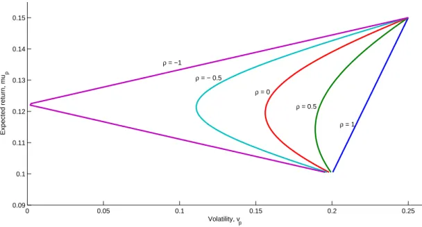
Clearly, the efficient portfolio frontier is an increasing and concave function of vp. It can be interpreted as a sort of “production function,” one that produces “expected returns” through inputs of “levels of risk” (see, e.g., Figure 1.1). The choice of which portfolio has effectively to be selected depends on the investor’s preference toward risk.
Example 1.1. Let the number of risky assets m = 2. In this case, we do not need to optimize anything, as the budget constraint, π1
w + π2
w = 1, pins down an unique relation between the portfolio expected return and the variance of the portfolio’s value. So we simply have, µp = E[w+w(π)]−w = π1
wb1+ π2
wb2, or,
µp =b1+ (b2−b1) π2
w v2
p =
1− π2 w
2 σ2
1+ 2
1− π2 w
π2
wσ12+
π2
w
2 σ2
0 0.05 0.1 0.15 0.2 0.25 0.09
0.1 0.11 0.12 0.13 0.14 0.15
Volatility, v
p
Expected return, mu
p
ρ = −1
ρ = − 0.5
ρ = 0
ρ = 0.5
ρ = 1
FIGURE 1.1. From top to bottom: portfolio frontiers corresponding toρ=−1,−0.5,0,0.5,1. Param-eters are set to b1 = 0.10, b2 = 0.15, σ1 = 0.20, σ2 = 0.25. For each portfolio frontier, the efficient
portfolio frontier includes those portfolios which yield the lowest volatility for a given expected return.
whence:
vp = 1 b2−b1
b2−µp
2 σ2
1+ 2
b2−µp µp−b1
ρσ1σ1 +
µp−b1
2 σ2
2
When ρ= 1,
µp =b1+
(b1−b2) (σ1−vp) σ2−σ1
.
In the general case, diversification pays when the asset returns are not perfectly positively correlated (see Figure 1.1). As Figure 1.1 reveals, it is even possible to obtain a portfolio that is less risky than than the less risky asset. Moreover, risk can be zeroed when ρ =−1, which corresponds to π1
w = σ2 σ2−σ1 and
π2 w =−
σ1
σ2−σ1 or, alternatively, to π1
w =− σ2 σ2−σ1 and
π2 w =
σ1 σ2−σ1.
Let us return to the general case. The portfolio in Eq. (1.9) can be decomposed into two components, as follows:
ˆ π(vp)
w =ℓ(vp) πd
w + [1−ℓ(vp)] πg
w, ℓ(vp)≡
βµp(vp)γ−β αγ −β2 ,
where
πd w ≡
Σ−1b β ,
πg w ≡
Hence, we see that πg
w is the global minimum variance portfolio, for we know from Eq. (1.10) that the minimum variance occurs at (vp, µp) = 1γ,
β γ
, in which case ℓ(vp) = 0.1 More generally, we can span any portfolio on the frontier by just choosing a convex combination of
πd w and
πg
w, with weight equal to ℓ(vp). It’s a mutual fund separation theorem.
1.1.4 The market portfolio
The market portfolio is the portfolio at which the CML in Eq. (1.6) and the efficient portfolio frontier in Eq. (1.11) intersect. In fact, the market portfolio is the point at which the CML is
tangent at the efficient portfolio frontier. For this reason, the market portfolio is also referred to as the “tangent” portfolio. In Figure 1.2, the market portfolio corresponds to the point M (the portfolio with volatility equal to vM and expected return equal toµM), which is the point at which the CML is tangent to the efficient portfolio frontier, AM C.2
As Figure 1.2 illustrates, the CML dominates the efficient portfolio frontier AM C. This is because the CML is the value of the investor’s problem, [1.P1], obtained using all the risky assets and the riskless asset, and the efficient portfolio frontier is the value of the investor’s problem, [1.P2], obtained using only all the risky assets.3 For the same reason, the CML and the efficient portfolio frontier can only be tangent with each other. For suppose not. Then, there would exist a point on the efficient portfolio frontier that dominates some portfolio on the CML, a contradiction. Likewise, the CML must have a portfolio in common with the efficient portfolio frontier - the portfolio that does not include the safe asset. Below, we shall use this insight to characterize, analytically, the market portfolio.
Why is the market portfolio called in this way? Figure 1.2 reveals that any portfolio on the CML can be obtained as a combination of the safe asset and the market portfolioM (a portfolio containing only the risky assets). An investor with high risk-aversion would like to choose a point such as Q, say. An investor with low risk-aversion would like to choose a point such asP, say. But no matter how risk averse an individual is, the optimal solution for him is to choose a combination of the safe asset and the market portfolio M. Thus, the market portfolio plays an instrumental role. It obviously does not depend on the risk attitudes of any investor - it is a mere convex combination of all the existing assets in the economy. Instead, the optimal course of action for any investor is to use those proportions of this portfolio that make his overall exposure to risk consistent with his risk appetite. It’s a two fund separation theorem.
The equilibrium implications if this separation theorem as follows. As we have explained, any portfolio can be attained by lending or borrowing funds in zero net supply, and in the portfolio M. In equilibrium, then, every investor must hold some proportions of M. But since in aggregate, there is no net borrowing or lending, one has that in aggregate, all investors must have portfolio holdings that sum up to the market portfolio, which is therefore the
value-1It is easy to show that the covariance of the global minimum variance portfolio with any other portfolio equalsγ−1. 2The existence of the market portfolio requires a restriction onr, derived in Eq. (1.12) below.
vM
CML
r
M µM
A
C
P
Q
Z
FIGURE 1.2.
weighted portfolio of all the existing assets in the economy. This argument is formally developed in the appendix.
We turn to characterize the market portfolio. We need to assume that the interest rate is sufficiently low to allow the CML to be tangent at the efficient portfolio frontier. The technical condition that ensures this is that the return on the safe asset be less than the expected return on the global minimum variance portfolio, viz
r < β
γ. (1.12)
LetπM be the market portfolio. To identifyπM, we note that it belongs toAM Cifπ⊤
M1m =w, where πM also belongs to the CML and, therefore, by Eq. (1.5), is such that:
πM w =
Σ−1(b−1mr) √
Sh ·vM. (1.13)
Therefore, we must be looking for the value vM that solves
w=1⊤mπM =w·1⊤mΣ−
1(b−1mr) √
Sh ·vM, i.e.
vM = √
Sh
β−γr. (1.14)
Then, we plug this value of vM into the expression for πM in Eq. (1.13) and obtain,4 πM
w = 1 β−γrΣ
−1(b
−1mr). (1.15)
Once again, the market portfolio belongs to the efficient portfolio frontier. Indeed, on the one hand, the market portfolio can not be above the efficient portfolio frontier, as this would contradict the efficiency of the AM C curve, which is obtained by investing in the risky assets only; on the other hand, the market portfolio can not be below the efficient portfolio frontier, for by construction, it belongs to the CML which, as shown before, dominates the efficient portfolio frontier. In the appendix, we confirm, analytically, that the market portfolio does indeed enjoy the tangency condition.
1.2 The CAPM
The Capital Asset Pricing Model (CAPM) provides an asset evaluation formula. In this section, we derive the CAPM through arguments that have the same flavor as the original derivation of Sharpe (1964). The first step is the creation of a portfolio including a proportion α of wealth invested in any asset i and the remaining proportion 1−α invested in the market portfolio. Mathematically, we are considering an α-parametrized portfolio, with expected return and volatility given by:
˜
µp ≡αbi+ (1−α)µM ˜
vp ≡(1−α)2σ2
M + 2(1−α)ασiM+α2σ2i
(1.16)
where we have definedσM ≡vM. Clearly, the market portfolio,M, belongs to theα-parametrized portfolio. By the Example 1.1, the curve in (1.16) has the same shape as the curve A′M i in Figure 1.3. The curve A′M i lies below the efficient portfolio frontier AM C. This is because the efficient portfolio frontier is obtained by optimizing a mean-variance criterion over all the existing assets and, hence, dominates any portfolio that only comprises the two assets iandM. Suppose, for example, that the A′M i curve intersects the AMC curve; then, a feasible combi-nation of assets (including some proportion α of the i-th asset and the remaining proportion 1−α of the market portfolio) would dominate AM C, a contradiction, given that AM C is the most efficient feasible combination of all the assets. On the other hand, the A′Mi curve has a point in common with the AM C, which isM, in correspondence ofα= 0. Therefore, the curve A′M i is tangent to the efficient portfolio frontier AM C at M, which in turn, as we already know, is tangent to the CML at M.
Let us equate, then, the two slopes of the A′M i curve and the efficient portfolio frontier AM C at M. We shall show that this condition provides a restriction on the expected returnbi on any asset i. Because (1.16) is, mathematically, an α-parametrized curve, we may compute its slope at M through the computation of d˜µpdα and d˜vp/dα, at α= 0. We have,
dµ˜p
dα =bi−µM, d˜vp
dα
α=0
=−−(1−α)σ 2
M + (1−2α)σiM +ασ2i|α=0 ˜
vp|α=0 = 1 σM
σiM−σ2M.
Therefore,
d˜µp(α) d˜vp(α)
α=0
= 1 bi−µM σM (σiM −σ
2 M)
vM
CML
r
M
A
C i
A’ µM
FIGURE 1.3.
On the other hand, the slope of the CML is (µM −r)/σM which, equated to the slope in Eq. (1.17), yields,
bi−r=βi(µM −r), βi ≡ σiM v2
M
, i= 1,· · · , m. (1.18)
Eq. (1.18) is the celebratedSecurity Market Line (SML). The appendix provides an alternative derivation of the SML. Assets with βi > 1 are called “aggressive” assets. Assets with βi < 1 are called “conservative” assets.
Note, the SML can be interpreted as a projection of the excess return on asseti (i.e. ˜bi−r) on the excess returns on the market portfolio (i.e. ˜bM −r). In other words,
˜bi−r=β
i(˜bM −r) +εi, i= 1,· · · , m. (1.19) The previous relation leads to the following decomposition of the volatility (or risk) related to the i-th asset return:
σ2i =β2ivM2 +var(εi), i= 1,· · · , m. The quantity β2iv2
M is usually referred to assystematic risk. The quantityvar(εi)≥0, instead, is what we term idiosyncratic risk. In the next section, we shall show that idiosyncratic risk can be eliminated through a “well-diversified” portfolio - roughly, a portfolio that contains a large number of assets. Naturally, economic theory does not tell us anything substantial about how important idiosyncratic risk is for any particular asset.
The CAPM can be usefully interpreted within a classical hedging framework. Suppose we hold an asset that delivers a return equal to ˜z - perhaps, a nontradable asset. We wish to hedge against movements of this asset by purchasing a portfolio containing a percentage of α in the market portfolio, and a percentage of 1−α units in a safe asset. The hedging criterion we wish to use is the variance of the overall exposure of the position, which we minimize by
minαvar[˜z−((1−α)r+α˜bM)]. It is straight forward to show that the solution to this basic problem is, ˆα≡ β˜z ≡ cov(˜z,˜bM)/v2
m. That is, the proportion to hold is simply the beta of the asset to hedge with the market portfolio.
The CAPM is a model for the required return for any asset and so, it is a very first tool we can use to evaluate risky projects. Let
V = value of a project = E(C +) 1 +rC ,
whereC+is future cash flow and rC is the risk-adjusted discount rate for this project. We have: E(C+)
V = 1 +rC
= 1 +r+βC(µM −r) = 1 +r+ cov
C+
V −1,xM˜
v2 M
(µM −r) = 1 +r+ 1
V
cov(C+,xM˜ ) v2
M
(µM −r) = 1 +r+ 1
Vcov
C+,xM˜ λ vM,
where λ≡ µM−r
vM , the unit market risk-premium.
Rearranging terms in the previous equation leaves:
V = E(C
+)− λ
vMcov(C
+,xM˜ )
1 +r . (1.20)
The certainty equivalent ¯C is defined as:
¯
C :V = E(C +) 1 +rC =
¯ C 1 +r,
or,
¯
C = (1 +r)V,
and using Eq. (1.20),
¯
C =EC+− λ vMcov
C+,xM˜ .
1.3 The APT
1.3.1 A first derivation
Suppose that them asset returns we observe are generated by the followinglinear factor model,
˜b
m×1 = ma×1+mB×k·kf×1 ≡a+cov(˜b, f)[var(f)] −1
whereaandB are a vector and a matrix of constants, andf is ak-dimensional vector of factors supposed to affect the asset returns, with k ≤ m. Let us normalize [var(f)]−1 =Ik
×k, so that B =cov(˜b, f). With this normalization, we have,
˜ b =a+
cov(˜b1, f) .. . cov(˜bm, f)
·f =a+
k
j=1cov(˜b1, fj)fj ..
.
k
j=1cov(˜bm, fj)fj
.
Next, let us consider a portfolioπ including the m risky assets. The return of this portfolio is,
π⊤˜b=π⊤a+π⊤Bf,
where as usual, π⊤1
m = 1. An arbitrage opportunity arises if there exists some portfolio π such that the return on the portfolio is certain, and different from the safe interest rater, i.e. if ∃π :π⊤B = 0 andπ⊤a=r. Mathematically, this is ruled out whenever∃λ∈Rk :a =Bλ+1mr. Substituting this relation into Eq. (1.21) leaves,
˜
b =1mr+Bλ+Bf =1mr+cov(˜b, f)λ+cov(˜b, f)f. Taking the expectation,
bi =r+ (Bλ)i =r+k
j=1cov(˜ bi, fj) ≡βi,j
λj, i= 1,· · · , m. (1.22)
The APT collapses to the CAPM, once we assume that the only factor affecting the returns is the market portfolio. To show this, we must normalize the market portfolio return so that its variance equals one, consistently with Eq. (1.22). So let ˜rM be the normalized market return, defined as ˜rM ≡v−M1˜bM, so that var(˜rM) = 1. We have,
˜
bi =a+βirM˜ , i= 1,· · · , m, where βi =cov(˜bi,rM˜ ) =vM−1cov(˜bi,˜bM). Then, we have,
bi =r+βiλ, i= 1,· · · , m. (1.23)
In particular, βM =cov(˜bM,rM˜ ) =vM−1var(˜bM) = vM, and so, by Eq. (1.23), λ= bM −r
vM ,
which is known as the Sharpe ratio for the market portfolio, or the market price of risk. By replacingβi =vM−1cov(˜bi,˜bM) and the expression for λ above into Eq. (1.23), we obtain,
bi =r+ cov(˜bi,˜bM) v2
M
(bM −r), i= 1,· · · , m.
This is simply the SML in Eq. (1.18).
1.3.2 The APT with idiosyncratic risk and a large number of assets
[Ross (1976), and Connor (1984), Huberman (1983).]
How can idiosyncratic risk be eliminated? Consider, for example, Eq. (1.19). Intuitively, we may form portfolios with a large number of assets, so as to make idiosyncratic risk negligible, by the law of large numbers. But would the beta-relation still hold, in this case? More in general, would the APT relation in Eq. (1.22) be still valid? The answer is in the affirmative, although it deserves some qualifications.
Consider the APT equation (1.21), and “add” a vector of idiosyncratic returns, ε, which are independent of f, and have mean zero and variance σ2
ε: ˜b=a+B·f +ε.
We wish to show that in the absence of arbitrage, to be defined below, it must be that the number of assets such that Eq. (1.22) does not hold, N(m) say, is bounded as m gets large, i.e.:
|ai−((Bλ)i+r)|>0, i= 1,· · · , N(m), (1.24) where
lim
m→∞N(m)<∞. (1.25)
In other words, we wish to show that in a “large” market, Eq. (1.22) does indeed hold for most of the assets, an approach close to that in Huang and Litzenberger (1988, p. 106-108).
By the same arguments leading to Eq. (1.1), the wealth generated by a portfolio of the assets satisfying (1.24), w+N(m) say, is,
w+
N(m)=π⊤N(m)
aN(m)−1N(m)r
+RwN(m)+π⊤N(m)
BN(m)f+εN(m)
,
where aN, BN and εN are (i) the vector of the expected returns, (ii) the return volatility (or factor exposures) matrix and (iii) the vector of idiosyncratic return components affecting these assets, and, finally, πN and wN are the portfolio and the initial wealth invested in these assets. In this context, we may define an arbitrage as the portfolio πN(m) that in the limit, as the number of all the existing assets m gets large, is riskless and yet delivers an expected return strictly larger than the safe interest rate, viz
lim m→∞
E[wN+(m)] wN(m)
> R, and lim
m→∞var[w +
N(m)]→0. (1.26) We want to show that this situation does not arises, under the condition in (1.25), thereby establishing that the linear APT relation in Eq. (1.22) is valid for most of the assets, in a large market.
So suppose the linear relation, aN−1Nr=BNλ, doesn’t hold. Then, there exists a portfolio π such that,
π⊤BN = 0 and π⊤(aN −1Nr)= 0. (1.27) Consider the portfolio:
ˆ
πN = 1
N ·sign
π⊤(aN −1Nr)
where π is as in (1.27). With this portfolio we have, clearly, that E[w+N] = ˆπ⊤N(aN −1Nr) + RwN > RwN, for each N, and even for N large. That is, limm→∞E[wN+(m)]/wN(m)> R, which is the first condition in (1.26). As regards the second condition in (1.26), we have that
var[w+
N] = ˆπ⊤N
BNBN⊤+σ2εIN×N
ˆ
πN =σ2εˆπ⊤NπˆN,
where the second equality follows by the first relation in (1.27). Clearly, limm→∞var[w+N(m)]→0 as N(m)→ ∞. Hence, in the absence of arbitrage, the condition in (1.25) must hold.
1.3.3 Empirical evidence
How to estimate Eq. (1.19)? Consider a slightly more general version of Eq. (1.19), where the safe interest rate is time-varying:
˜
bi,t−rt=βi(˜bM,t−rt) +εi,t, i= 1,· · · , m,
where εi,t denote “time-series residuals.” Fama and MacBeth (1973) consider the following procedure. In a first step, one obtains estimates of the exposures to the market, ˆβi say, for all stocks, using, for example, monthly returns, and approximating the market portfolio with some broad stock market index.5 In a second step, one runs cross-sectional regressions, one for each month,
˜
bi,t−rt=αit+λtβˆi+ηi,t, t= 1,· · · , T,
where T is the sample size and ηi,t denote “sectional residuals.” The time-series of cross-sectional estimates of the intercept αi,t and the price of risk λt, ˆαi,t and ˆλt say, are, then, used to make statistical inference. For example, time-series averages and standard errors of ˆαi,t and ˆ
λt lead to point estimates and standard errors for αi,t and λt. If the CAPM holds, estimates of αi should not be significantly different from zero.
Chen, Roll and Ross (1986) use the Fama-MacBeth two-step procedure to estimate a multi-factor APT model, such as that in Section 1.3. They identify “macroeconomic forces” driving asset returns with the innovations in variables such as the term spread, expected and unex-pected inflation, industrial production growth, or the corporate spread. They find that these sources of variation in the cross-section of asset returns are significantly priced.
5In tests of the CAPM, one uses proxies of the market portfolio, such as, say, the S&P 500. However, the market portfolio is unobservable. Roll (1977) points out that as a result, the CAPM is inherently untestable, as any test of the CAPM is a joint test of the model itself and of the closeness of the proxy to the market portfolio.
1.4 Appendix 1: Some analytical details for portfolio choice
We derive Eq. (1.9), which provides the solution for the portfolio choice when the space choice does not include a safe asset. We derive the solution by proceeding with two programs: (i) the primal program [1.P2] in the main text, which consists in maximizing the portfolio expected return, given a certain level of the variance of the portfolio’s value; and (ii) a dual program, to be introduced below, by which one minimizes the variance of the portfolio’s value, given a certain level of the portfolio expected return.
1.4.1 The primal program
Given Eq. (1.8), the Lagrangian function associated to [1.P2] is,
L=π⊤b+w−ν1(π⊤Σπ−w2·v2p)−ν2(π⊤1m−w),
where ν1 and ν2 are two Lagrange multipliers. The first order conditions are,
ˆ
π = 1
2ν1Σ
−1(b−ν
21m), πˆ⊤Σˆπ =w2·vp2, ˆπ⊤1m =w. (1A.1)
Using the first and the third conditions, we obtain,
w=1⊤mˆπ= 1 2ν1(
1⊤mΣ−1b
≡β
−ν21⊤mΣ−11m
≡γ
)≡ 21ν
1(β−ν2γ).
We can solve for ν2, obtaining,
ν2= β−2wν1
γ .
By replacing the solution forν2 into the first condition in (1A.1) leaves,
ˆ
π= w
γΣ−
11 m+ 1
2ν1Σ −1
b−βγ1m
. (1A.2)
Next, we derive the value of the program [1.P2]. We have,
Ew+(ˆπ)−w= ˆπ⊤b= w
γ1⊤mΣ−
1b
≡β
+ 1 2ν1(b
⊤Σ−1b
≡α
−βγ1⊤mΣ−1b
≡β
) = w
γβ+
1 2ν1
α−β 2 γ . (1A.3)
It is easy to check that
varw+(ˆπ) = w2·vp2
= ˆπ⊤Σˆπ = w γ1 ⊤ mΣ−1+
1 2ν1
b⊤−β
γ1
⊤ m
Σ−1 w
γ1m+
1 2ν1
b− β
γ1m
= w 2 γ + 1 2ν1
2 α−β 2 γ . (1A.4)
Let us gather Eqs. (1A.3) and (1A.4),
µp(vp)≡ E[w
+(ˆπ)]−w
w =
β
γ +
1 2ν1w
α−β
2
γ
vp2=
1
γ +
1 2ν1w
2
α−β
2
γ
where we have emphasized the dependence of µp on vp, which arises through the presence of the
Lagrange multiplierν1.
Let us rewrite the first equation in (1A.5) as follows, 1
2ν1w =
αγ−β2−1γµp(vp)−β. (1A.6)
We can use this expression forν1 to express ˆπ in Eq. (1A.2) in terms of the portfolio expected return,
µp(vp). We have,
ˆ
π
w =
Σ−11 m
γ +
αγ−β2−1γµp(vp)−β
Σ−1b−Σ−
1β
γ 1m
.
By rearranging terms in the previous equation, we obtain Eq. (1.9) in the main text. Finally, we substitute Eq. (1A.6) into the second equation in (1A.5), and obtain:
v2p = 1
γ 1 +
αγ−β2−1γµp(vp)−β2 !
,
which is Eq. (1.10) in the main text. Note, also, that the second condition in (1A.5) reveals that,
1 2ν1w
2
= γv
2 p−1
αγ−β2.
Given thatαγ−β2>0, the previous equation confirms the properties of theglobal minimum variance portfolio stated in the main text.
1.4.2 The dual program
We now solve the dual program, defined as follows, ˆ
π = arg min
π∈Rmvar
w+(π)
w
s.t.Ew+(π)=Ep andw=π⊤1m, [1A.P2-dual]
for some constantEp. The first order conditions are
ˆ
π
w =
ν1w
2 Σ
−1b+ν2w
2 Σ
−11
m ; πˆ⊤b=Ep−w ; w= ˆπ⊤1m; (1A.7)
where ν1 and ν2 are two Lagrange multipliers. By replacing the first condition in (8A.14) into the
second one,
Ep−w= ˆπ⊤b=w2(ν1
2 b
⊤Σ−1b
≡α
+ν2 2 1
⊤ mΣ−1b
≡β
)≡w2ν1
2 α+
ν2
2 β
. (1A.8)
By replacing the first condition in (8A.14) into the third one,
w= ˆπ⊤1m=w2(ν1
2 b
⊤Σ−11 m
≡β
+ ν2 2 1
⊤
mΣ−11m
≡γ
)≡w2ν1
2 β+
ν2
2 γ
. (1A.9)
Next, letµp ≡ Ep−w
w . By Eqs. (1A.8) and (1A.9), the solutions forν1 and ν2 are,
ν1w
2 =
µpγ−β
αγ−β2 ;
ν2w
2 =
α−βµp
αγ−β2
Therefore, the solution for the portfolio in Eq. (8A.14) is, ˆ
π
w =
γµp−β
αγ−β2Σ
−1b+α−βµp
αγ−β2Σ
−11 m.
Finally, the value of the program is,
var
w+(ˆπ)
w
= 1
w2πˆ⊤Σˆπ =
1
wπˆ
⊤µpγ−β
αγ−β2b+
1
wπˆ
⊤α−µpβ
αγ−β21m=
γµ2p−2βµp+α
αγ−β2 =
(γµp−β)2
(αγ−β2)γ+
1
γ,
1.5 Appendix 2: The market portfolio
1.5.1 The tangent portfolio is the market portfolio
Let us define the market capitalization for any assetias the value of all the assetsithat are outstanding in the market, viz
Capi≡¯θiSi, i= 1,· · ·, m,
where ¯θi is the number of assets i outstanding in the market. The market capitalization of all the
assets is simply
CapM ≡ m
i=1
Capi.
The market portfolio, then, is the portfolio with relative weights given by, ¯
πM,i≡ Capi
CapM
, i= 1,· · ·, m.
Next, suppose there areN investors and that each investorjhas wealthwj, which he invests in two
funds, a safe asset and the tangent portfolio. Let wfj be the wealth investorj invests in the safe asset and wj−wfj the remaining wealth the investor invests in the tangent portfolio. The tangent portfolio
is defined as ¯πT ≡
πT
wj
, for someπT solution to [1.P2], and is obviously independent of wj (see Eq.
(1.15) in the main text). The equilibrium in the stock market requires that CapM ·π¯M =
N
j=1
wj−wjf
¯
πT =
N
j=1
wj·π¯T = CapM ·π¯T.
where the second equality follows because the safe asset is in zero net supply and, hence,Nj=1wfj = 0; and the third equality holds because all the wealth in the economy is invested in stocks, in equilibrium.
1.5.2 Tangency condition
We check that the CML and the efficient portfolio frontier have the same slope in correspondence of the market portfolio. Let us impose the following tangency condition of the CML to the efficient portfolio frontier in Figure 1.2,AMC, at the pointM:
√
Sh = αγ−β
2
γµM −βvM. (1A.10)
The left hand side of this equation is the slope of the CML, obtained through Eq. (1.6). The right hand side is the slope of the efficient portfolio frontier, obtained by differentiating µp(v) in the expression
for the portfolio frontier in Eq. (1.11), and settingv=vM in
dµp(v)
dv = (γv
2−1)−1αγ−β2v= αγ−β2
γµp(v)−β
v,
and where the second equality follows, again, by Eq. (1.11). By Eqs. (1A.10) and (1.14), we need to show that,
γµM −β
αγ−β2 =
1
β−γr.
By pluggingµM =r+
√
Sh·vM into the previous equality and rearranging terms,
vM =
√
Sh
β−γr,
where we have made use of the equality Sh =α−2βr+γr2, obtained by elaborating on the definition
1.6 Appendix 3: An alternative derivation of the SML
The vector of covariances of the masset returns with the market portfolio are:
cov(˜x,x˜M) =cov
˜
x,x˜·πwM= ΣπM
w =
1
β−γr(b−1mr), (1A.11)
where we have used the expression for the market portfolio given in Eq. (1.15). Next, premultiply the previous equation by π⊤M
w to obtain:
v2M =
π⊤M
w Σ
πM
w =
π⊤M w
1
β−γr(b−1mr) =
1
(β−γr)2Sh, (1A.12)
orvM = √
Sh
β−γr, which confirms Eq. (1.14).
Let us rewrite Eq. (1A.11) component by component. That is, fori= 1,· · · , m,
σiM ≡cov(˜xi,x˜M) = 1
β−γr(bi−r) = vM
√
Sh(bi−r) =
vM2
µM −r (bi−r),
where the last two equalities follow by Eq. (1A.12) and by the relation, √Sh = µM−r
vM . By rearranging
terms, we obtain Eq. (1.18).
1.7 Appendix 4: Broader definitions of risk - Rothschild and Stiglitz theory
The papers are Rothschild and Stiglitz (1970, 1971). Notation, any variable with a tilde is a random variable. Let us consider the following definition of stochastic dominance:
Definition A.1 (Second-order stochastic dominance). ˜x2 dominates x˜1 if, for each utility function
u satisfying u′ ≥0,we have also that E[u(˜x2)]≥E[u(˜x1)].
We have:
Theorem A.2.The following statements are equivalent:
a) ˜x2 dominates x˜1, or E[u(˜x2)]≥E[u(˜x1)];
b) ∃ random variable η >0 : ˜x2 = ˜x1+η;
c) ∀x >0, F1(x)≥F2(x).
Proof.We provide the proof when the support is compact, say [a, b]. First, we show thatb)⇒c). We have: ∀t0∈[a, b], F1(t0)≡Pr (˜x1≤t0) = Pr (˜x2 ≤t0+η)≥Pr (˜x2≤t0)≡F2(t0). Next, we show
that c)⇒a). By integrating by parts,
E[u(x)] =
" b a
u(x)dF(x) =u(b)−
" b a
u′(x)F(x)dx,
where we have used the fact that: F(a) = 0 and F(b) = 1. Therefore,
E[u(˜x2)]−E[u(˜x1)] = " b
a
u′(x) [F1(x)−F2(x)]dx.
Finally, it is easy to show that a)⇒b).
Next, we turn to the definition of “increasing risk”:
Definition A.3. ˜x1 is more risky than x˜2 if, for each function u satisfying u′′ <0,we have also
that E[u(˜x1)]≤E[u(˜x2)]for x˜1 and x˜2 having the same mean.
This definition of “increasing risk” does not rely on the sign of u′. Furthermore, if var(˜x1) >
var(˜x2), ˜x1 is not necessarily more risky than ˜x2, according to the previous definition. The standard
counterexample is the following one. Let ˜x2= 1 w.p. 0.8, and 100 w.p. 0.2. Let ˜x1 = 10 w.p. 0.99, and
1090 w.p. 0.01. We have, E(˜x1) = E(˜x2) = 20.8, but var(˜x1) = 11762.204 and var(˜x2) = 1647.368.
However, consider u(x) = logx. Then, E(log (˜x1)) = 2.35> E(log (˜x2)) = 0.92. It is easily seen that
in this particular example, the distribution functionF1 of ˜x1 “intersects”F2, which is in contradiction
with the following theorem.
Theorem A.4.The following statements are equivalent:
a) ˜x1 is more risky than x˜2;
b) ˜x1 has more weight in the tails than x˜2,i.e. ∀t, #−∞t [F1(x)−F2(x)]dx≥0;
c) ˜x1 is a mean preserving spread of x˜2, i.e. there exists a random variable ǫ : ˜x1 has the same
Proof. Let us begin withc)⇒a). We have,
E[u(˜x1)] = E[u(˜x2+ǫ)]
= E[E(u(˜x2+ǫ)|x˜2 =x2)]
≤ E[u(E( ˜x2+ǫ|x˜2=x2))]
= E[u(E( ˜x2|x˜2 =x2))]
= E[u(˜x2)].
As regards a)⇒b), we have that:
E[u(˜x1)]−E[u(˜x2)] = " b
a
u(x) [f1(x)−f2(x)]dx
= u(x) [F1(x)−F2(x)]|ba− " b
a
u′(x) [F1(x)−F2(x)]dx
=−
" b a
u′(x) [F1(x)−F2(x)]dx
=−
u′(x)F¯1(x)−F¯2(x)ba− " b
a
u′′(x)F¯1(x)−F¯2(x)dx
=
" b a
u′′(x)F¯1(x)−F¯2(x)dx−u′(b)F¯1(b)−F¯2(b),
where ¯Fi(x) =#axFi(u)du. Now, ˜x1 is more risky than ˜x2means thatE[u(˜x1)]< E[u(˜x2)] foru′′<0.
By the previous relation, then, ¯F1(x) >F¯2(x). Finally, see Rothschild and Stiglitz (1970) p. 238 for
the proof of b)⇒c).
References
Chen, N-F., R. Roll and S.A. Ross (1986): “Economic Forces and the Stock Market.”Journal of Business 59, 383-403.
Connor, G. (1984): “A Unified Beta Pricing Theory.”Journal of Economic Theory 34, 13-31.
Fama, E.F. and J.D. MacBeth (1973): “Risk, Return, and Equilibrium: Empirical Tests.”
Journal of Political Economy 38, 607-636.
Huang, C-f. and R.H. Litzenberger (1988): Foundations for Financial Economics. New York: North-Holland.
Huberman, G. (1983): “A Simplified Approach to Arbitrage Pricing Theory.”Journal of Eco-nomic Theory 28, 1983-1991.
Markovitz, H. (1952): “Portfolio Selection.” Journal of Finance 7, 77-91.
Roll, R. (1977): “A Critique of the Asset Pricing Theory’s Tests Part I: On Past and Potential Testability of the Theory.” Journal of Financial Economics 4, 129-176.
Ross, S. (1976): “Arbitrage Theory of Capital Asset Pricing.” Journal of Economic Theory
13, 341-360.
Rothschild, M. and J. Stiglitz (1970): “Increasing Risk: I. A Definition.”Journal of Economic Theory 2, 225-243.
Rothschild, M. and J. Stiglitz (1971): “Increasing Risk: II. Its Economic Consequences.” Jour-nal of Economic Theory 5, 66-84.
The CAPM in general equilibrium
2.1 Introduction
This chapter develops the general equilibrium foundations to the CAPM, within a framework that abstracts from the production sphere of the economy. For this reason, we usually refer the resulting model to as the “Consumption-CAPM.” First, we review the static model of general equilibrium, without uncertainty. Then, we illustrate the economic rationale behind the existence of financial assets in an uncertain world. Finally, we derive the Consumption-CAPM.
2.2 The static general equilibrium in a nutshell
We consider an economy with n agents and m commodities. Let wij denote the amount of the i-th commodity the j-th agent is endowed with, and let wj = [w
1j,· · · , wmj]. Let the price vector be p = [p1,· · · , pm], where pi is the price of the i-th commodity. Let wi = nj=1wij be the total endowment of the i-th commodity in the economy, and W = [w1,· · ·, wm] the corresponding endowments bundle in the economy.
The j-th agent has utility function uj(c1j,· · ·, cmj), where (cij)mi=1 denotes his consumption bundle. We assume the following standard conditions for the utility functions uj:
Assumption 2.1 (Preferences). The utility functions uj satisfy the following properties: (i) Monotonicity; (ii) Continuity; and (iii) Quasi-concavity: uj(x) ≥ uj(y), and ∀α ∈ (0,1), uj(αx+ (1−α)y)> uj(y) or, ∂c∂uijj (c1j,· · ·, cmj)≥0 and ∂
2u
j
∂c2
ij(c1j,· · · , cmj)≤0.
LetBj(p1,· · · , pm) = {(c1j,· · · , cmj) :mi=1picij ≤
m
i=1piwij ≡Rj}, a bounded, closed and convex set, hence a convex set. Each agent maximizes his utility function subject to the budget constraint:
max {cij}
This problem has certainly a solution, for Bj is compact set and by Assumption 2.1, uj is continuous, and a continuous function attains its maximum on a compact set. Moreover, the Appendix shows that this maximum is unique.
The first order conditions to [P1] are, for each agent j,
∂uj
∂c1j
p1 =
∂uj
∂c2j
p2
=· · ·= ∂uj
∂cmj
pm m
i=1
picij = m
i=1 piwij
(2.1)
These conditions form a system of m equations with m unknowns. Let us denote the solution to this system with [ˆc1j(p, wj),· · · ,ˆcmj(p, wj)]. The total demand for thei-th commodity is,
ˆ
ci(p, w) = n
j=1 ˆ
cij(p, wj), i= 1,· · · , m.
We emphasize the economy we consider in this chapter is one that completely abstracts from production. Here, prices are the key determinants of how resources are allocated in the end. The perspective is, of course, radically different from that taken by the Classical school (Ricardo, Marx and Sraffa), for which prices and resources allocation cannot be disentangled from the production side of the economy. In the next chapter and more advanced parts of the lectures, we consider the asset pricing implications of production, following the Neoclassical perspective.
2.2.1 Walras’ Law
Let us plug the demand functions of the j-th agent into the constraint of [P1], to obtain,
∀p, 0 = m
i=1
picij(p, wˆ j)−wij. (2.2)
Next, define the total excess demand for the i-th commodity as ei(p, w) ≡ ˆci(p, w)−wi. By aggregating the budget constraint across all the agents,
∀p, 0 = n
j=1 m
i=1
picij(p, wˆ j)−wij= m
i=1
piei(p, w).
The previous equality is the celebrated Walras’ law.
Next, multiplypbyλ ∈R++. Since the constraint to [P1] does not change, the excess demand functions are the same, for each value of λ. In other words, the excess demand functions are homogeneous of degree zero in the prices, or ei(λp, w) = ei(p, w), i = 1,· · · , m. This property of the excess demand functions is also referred to as absence of monetary illusion.
2.2.2 Competitive equilibrium
Acompetitive equilibrium is a vector ¯pinRm