Distributed Brillouin fiber sensor assisted by first order Raman amplification

Texto completo

(1)> REPLACE THIS LINE WITH YOUR PAPER IDENTIFICATION NUMBER (DOUBLE-CLICK HERE TO EDIT) <. 1. Distributed Brillouin fiber sensor assisted by first-order Raman amplification Félix Rodríguez-Barrios, Sonia Martín-López, Ana Carrasco-Sanz, Pedro Corredera, Juan Diego Ania-Castañón, Luc Thévenaz and Miguel González-Herráez Abstract— Distributed optical fiber Brillouin sensors provide innovative solutions for the monitoring of temperature and strain in large structures. The effective range of these sensors is typically of the order of 20-30 km, which limits their use in certain applications in which the distance to monitor is larger. In this work, we have developed a new technique to significantly extend the measurement distance of a distributed Brillouin Optical Time-Domain Analysis (BOTDA) sensor. Distributed Raman Amplification in the sensing fiber provides the means to enhance the operating range of the setup. Three Raman pumping configurations are theoretically and experimentally investigated: co-propagating, counter-propagating and bi-directional propagation with respect to the Brillouin pump pulse. We show that some of the amplification schemes tested can extend the measurement range and improve the measurement quality over long distances. Index Terms— Brillouin scattering, distributed fiber optic sensor, Raman scattering, strain sensor, temperature sensor. I. I. INTRODUCTION. N recent years, fiber optic sensors have attracted great interest thanks to their unique properties: small size and weight, immunity to electromagnetic noise, environmental ruggedness and chemically inert nature, among others. This kind of sensors is very interesting for the monitoring of civil infrastructures, particularly when such infrastructures are located in electrically noisy environments or when the distance to be monitored is long. Distributed sensors represent. Manuscript received December 17, 2009. This work was supported in part by the Spanish Ministerio de Ciencia e Innovación through projects TEC200914423-C02-01, TEC2009-14423-C02-02 and TEC2008-05791, the Ministerio de Fomento through project MIFFO (FOM-07/77), the support from CSIC through the I3P Post-Doc program, and the support from the Comunidad Autonoma de Madrid through project FACTOTEM2 (S2009/ESP-1781). F. Rodríguez-Barrios, S. Martín-López and P. Corredera are with the Instituto de Fisica Aplicada, Consejo Superior de Investigaciones Cientificas (CSIC), 28006 Madrid, Spain. (e-mail: felix@ifa.cetef.csic.es). A. Carrasco-Sanz is with the Departamento de Optica, Facultad de Ciencias, Universidad de Granada, 18071 Granada, Spain. J. D. Ania-Castañón is with the Instituto de Optica, Consejo Superior de Investigaciones Cientificas (CSIC), 28006 Madrid, Spain L. Thévenaz is with the Institute of Electrical Engineering, Ecole Polytechnique Fédérale de Laussane. STI-GR Station 11, CH-1015, Laussane, Switzerland. M. González-Herráez is with the Departamento de Electronica, Universidad de Alcala. Edificio Politecnico, 28871 Alcala de Henares, Madrid, Spain.. a particular kind of fiber optic sensors which allows for the simultaneous monitoring of physical parameters at different points along the fiber, that is, a system in which the whole fiber behaves as a sensor. In 1989, Brillouin Optical TimeDomain Analysis (BOTDA), a distributed sensing technique based on Brillouin scattering in optical fibre, was proposed and demonstrated [1]-[3] based upon the possibility of relating variations of strain and temperature in the optical waveguide to variations in the peak gain frequency for Brillouin scattering. The distributed measurement of strain is of great interest to guarantee the integrity of optical fibers, as well as to monitor civil structures such as bridges, tunnels, buildings, pipelines, etc., to which optical fibers can be attached [4]. BOTDA sensors allow, therefore, a continuous monitoring of temperature and/or strain in an optical fiber [5]-[10]. The measurement range of this kind of systems is in all cases lower than 50 km [11] and generally limited to 20-30 km, with a spatial resolution between 1-2 meters. The measurement range limitation is basically due to the fiber attenuation, which is about 0.2 dB/km in modern optical fibers at a wavelength of 1.5 µm. The losses in the fiber cause a drop of signal contrast with distance and a growth in the measurement uncertainty, as a simple result of the pump power reduction that critically scales the actual gain. The sensor resolution has also an impact on the achievable measurement range. While it is desirable to have the highest possible resolution, this requires the use of short optical pulses, so the effective distance for amplification is reduced accordingly, which increases the difficulty in detection because the signal-to-noise ratio (SNR) is low. For this reason it becomes necessary to design each sensing scheme with an eye on its specific application. Depending on system requirements, it might be more convenient to use short pulses for increased resolution, or longer pulses for increased range. Several studies have been realized to extend the system resolution without impairing the measurement range [12], basically relying on signal processing methods. Other studies have concentrated on increasing the measurement range by trying to compensate the fiber loss using distributed Raman amplification. Raman amplification induces a distributed gain along the fiber that compensates for the intrinsic fiber loss and thus maintains the pump power to a level to secure a sufficient gain. In these studies, spontaneous Brillouin scattering sensors have been used [13]-[16]. However, to the best of our knowledge, no attempt to use Raman assistance in BOTDA sensors has been developed. In.

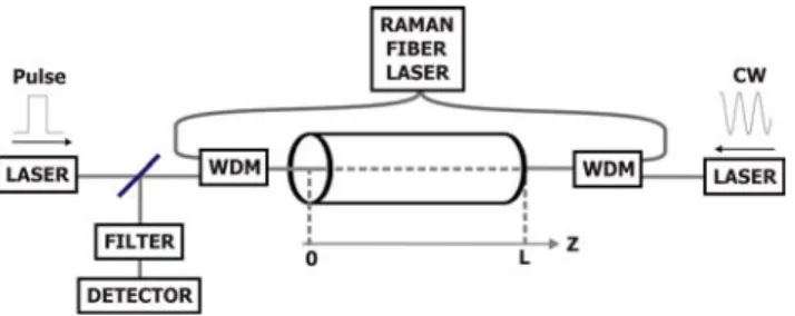
(2) > REPLACE THIS LINE WITH YOUR PAPER IDENTIFICATION NUMBER (DOUBLE-CLICK HERE TO EDIT) < this paper we investigate the use of Raman amplification for the improvement of the measurement range in BOTDA sensors. We explore three different Raman pumping configurations: counter-propagating, co-propagating and bidirectional pumping with respect to the Brillouin pump pulse. We show that in some of these configurations, the assistance of Raman amplification allows monitoring longer interaction distances, although special attention to the issue of Relative Intensity Noise (RIN) transfer from the Raman pump has to be paid. A measurement range of 75 km with a spatial resolution of 2 meters is achieved, demonstrating a marked improvement with respect to the conventional BOTDA setup. This paper is organized as follows. In Section II, some basic concepts of BOTDA technology are reviewed, with special emphasis on the parameters to pay attention in our study. In Section III, we show the theoretical model of Raman-assisted distributed Brillouin sensor; in Section IV, we depict the experimental setup that has been used for our demonstration. In Section V we present the theoretical and experimental results obtained comparing the Raman-assisted configurations with respect to the non-assisted one. These results show that it is possible to obtain an improved performance over conventional BOTDA in all the Raman-assisted BOTDA configurations shown. Section VI shows some preliminary hot-spot detection tests that demonstrate the feasibility of using the proposed setup as a long-range sensor. Finally, in Section VII we draw the essential conclusions of our study. II. BOTDA ASSISTED BY RAMAN Stimulated Brillouin Scattering (SBS) is a nonlinear effect that takes place very efficiently in optical fibers [17]. When pumping a single-mode optical fiber with an intense coherent light source centered at frequency f0, SBS manifests as a narrowband amplification of a counter-propagating beam around f0-υB. υB is known as the Brillouin shift of the fiber. The BOTDA technology takes root in the change of the Brillouin shift with different physical parameters. More specifically, it is possible to measure any kind of physical magnitude that produces a variation of the acoustic velocity or the refractive index inside the optical fiber [18], since the expression for υB is:. νB =. 2nva. λ. (1). where n is the refractive index of the optical fiber, va is the acoustic velocity along the fiber and λ is the pump wavelength. Strain and temperature are the most typical physical magnitudes monitored using this effect. The way to make this sensor distributed is to read the value of Brillouin shift along the fiber, that is, to determine the Brillouin shift at each position in the fiber. To do this, an optical time-domain analysis has to be performed, as shown in Fig. 1. BOTDA systems use two different counter-propagating singlefrequency light beams in the fiber. One of these light beams. 2. (centered at f0) is pulsed and is meant to generate some amplification on the probe; we call this signal pump wave. The other one (centered around f0-υB) is a continuous wave, called probe wave, that will be locally amplified by the pump pulse through SBS. As the pump pulse travels down the fiber, it will induce a different amplification on the probe depending on the Brillouin shift. The local amplification of the probe wave will yield a time-dependent variation of the detected probe signal at the pump end (see Fig. 1). The amplification at each point will be maximized when the pump-probe frequency separation is exactly the Brillouin shift at that point. By scanning for this maximum at all the positions, one can obtain a map of the Brillouin shift of the fiber across its whole length. Assuming small gain, the signal change recorded in the monitoring end will be ∆PB-(z)=G(ν,z)·PB-(z), where G(ν,z)=(gB(ν,z)/Aeff)·PB+(z)·∆z. PB+(z) and PB-(z) are the pump and probe wave powers, respectively, gB(ν,z) is the Brillouin gain coefficient (dependent on the position and the pumpprobe frequency separation ν), Aeff is the effective area of the fiber and ∆z is the pump pulse width. This notation assumes that the pump wave is introduced at position Z = 0 in the fiber and propagates in the +Z direction, whereas the probe wave is introduced at Z = L and propagates in the –Z direction. As mentioned before, the goal of BOTDA systems is to determine the Brillouin shift for each position. This is done by sweeping the frequency difference ν so as to maximize the gain G for each position. This determines correctly the Brillouin shift for each position unless pump depletion is relevant (this is, unless PB+(z) also depends on ν). Thus, in order to operate the setup correctly, it is indispensable to avoid any Brillouin pump depletion. This imposes strict limits in the Brillouin pump power used: if the Brillouin pump power is too low, the gain will be low and the contrast will be poor; if the pump power is too high, pump depletion will bias the correct determination of the Brillouin shift. Similar restrictions apply if we consider the probe power. To improve the dynamic range of the BOTDA we propose to introduce Raman pumping on one or both sides of the sensing fiber, as shown in Fig. 1. WDM couplers should allow maximizing the efficiency of the Raman pumping. By means of this amplification we transfer power both to the pump and probe waves. The objective of this study is to determine which pumping configuration provides the largest increase in the dynamic range and enables the longest measurement distance: co-propagating, counter-propagating or bi-directional propagation of the Raman pump with respect to the Brillouin pump wave..

(3) > REPLACE THIS LINE WITH YOUR PAPER IDENTIFICATION NUMBER (DOUBLE-CLICK HERE TO EDIT) <. Fig. 1. General configuration of BOTDA assisted by Raman amplification. III. THEORETICAL MODEL OF RAMAN-ASSISTED DISTRIBUTED BRILLOUIN SENSOR The goal of this section is to provide a theoretical model of the Raman-assisted BOTDA, shown in Fig. 1. Distributed Raman amplification, much like stimulated Brillouin scattering, uses the whole fiber span as an amplifier, in which energy from one or several high-power CW pumps is transferred to a signal propagating at longer wavelengths. The characteristic flat-gain region for Raman amplification in silica fibers offers a bandwidth of several nanometers, with a characteristic frequency shift of approximately 13 THz, orders of magnitude above that of Brillouin scattering. This means that, from the point of view of a Raman pump situated at about 1455 nm, the Brillouin pump and probe in the region of 1550 nm can be treated as being effectively at the same wavelength. From now on, we will refer to the case in which the Raman pump propagates in opposite direction to the Brillouin pump pulse (from right to left in the diagram in Fig. 1) as the counter-propagating configuration; to the case in which the Raman pump propagates with the Brillouin pump pulse as the co-propagating configuration; and to the case in which we have Raman pumps propagating in both directions as the bidirectional configuration. If we consider the system from the point of view of its steady-state equations, neglecting amplified spontaneous emission and Rayleigh backscattering noise, the evolution of both Raman pumps powers along the optical fiber can be obtained by solving the following coupled equations (2) and (3): dPP+ ( z ) ν = −α P PP+ ( z ) − g R P PP+ ( z ) PB+ ( z ) + PB− ( z ) dz νB. ]. (2). ν dPP− ( z ) = +α P PP− ( z ) + g R P PP− ( z ) PB+ ( z ) + PB− ( z ) νB dz. (3). [ [. ]. where PP± are the powers of the forward (+) or backward (– ) propagating Raman pumps; αP is the fiber optic attenuation at the wavelength of the Raman pump: 1455 nm; gR is Raman gain at 1550 nm. On the other hand, the Brillouin pump power along the optical fiber can be obtained using equation (4). dPB+ (z ) = −α B PB+ (z ) + g R PB+ (z ) PP+ (z ) + PP− (z ) dz − g B PB+ (z )PB− (z ). [. ]. (4). 3. where PB+ is the Brillouin pump power along the optical fiber; αB is the fiber optic attenuation at 1550 nm; gB is the Brillouin gain coefficient evaluated when the pump-probe frequency difference equals the Brillouin shift. We evaluate this case because it is the case in which the Brillouin pump depletion is the highest (significant pump depletion should be avoided to make correct measurements, as mentioned before). Finally, the evolution of the probe wave power along the optical fiber can be obtained using equation (5). dPB− (z ) = α B PB− ( z ) − g B PB+ (z )PB− ( z ) dz − g R PB− ( z ) PP+ ( z ) + PP− (z ). [. (5). ]. where PB- is the probe wave power. To provide an analytical solution to the evolution of all the waves in the setup, we can consider the Brillouin pump power and the probe wave power negligible with respect to the Raman pump powers in equations (2) and (3). Actually these two powers are approximately two orders of magnitude larger than those involved in the Brillouin interaction, hence we can neglect depletion effects. We can then approximate these equations as follows: dPP+ (z ) = −α P PP+ (z ) dz. (6). dPP− (z ) = +α P PP− (z ) dz. (7). Additionally, under the assumption that there is no Brillouin pump depletion we can approximate equation (5) this way: dPB+ ( z ) = −α B PB+ (z ) + g R PB+ (z ) PP+ ( z ) + PP− ( z ) dz. [. ]. (8). Finally, we can solve these equations to obtain analytical solutions for both Raman pump powers and for the Brillouin pump power: PP+ ( z ) = PP+ (0 ) ⋅ exp(− α P · z ). (9). P (z ) = P (L ) ⋅ exp(α P ·( z − L )) − P. − P. PB+ ( z ) = PB+ (0 ) ⋅ exp( PP+ (0 )g R. αP. P (0 )g R + P. αP. P (L )g R − P. exp(− α P z ) − − α B z). αP. exp(α P ( z − L )) −. PP− (L )g R. αP. (10). exp(− α P L ) +. (11).

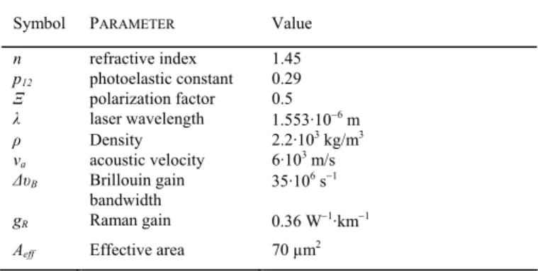
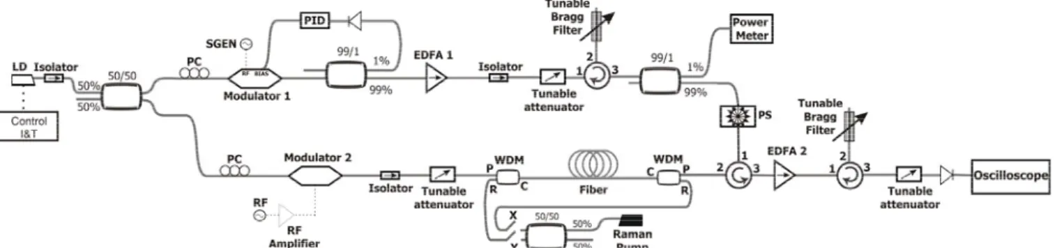
(4) > REPLACE THIS LINE WITH YOUR PAPER IDENTIFICATION NUMBER (DOUBLE-CLICK HERE TO EDIT) < PP− (L )g R. 4. power. The second approximation is to solve the differential equation under the assumption that the Brillouin pump power αP is constant with the distance, using as this constant value the + + PP (0 )g R P (0 )g R averaged power along the fiber, obtained through equation exp(− α P L ) + P exp(− α P z ) − αP αP (12) (11). The last approach is to resort to the numerical PP− (L )g R calculation of the integral in equation (12). We have computed exp(α P (z − L )) − all of these possible solutions and, using realistic values for αP the signal and probe powers, it is possible to conclude that + − P (0 )g R PP (L )g R − PB+ (0 )g B exp( P ·exp(− α P L )) ⋅ neglecting the last term in equation (12) yields a good αP αP estimation of the probe wave power along the optical fiber. z PP− (L )g R PP+ (0 )g R This approximation makes our model simpler and, as we will ∫L exp( α P ·exp(α P (z − L )) − α P ·exp(− α P z ) − α B z )) see in section V, the results are consistent with the experiment. + – + – where PP (0), PP (L), PB (0) and PB (L) are the boundary IV. EXPERIMENTAL SETUP conditions given by the optical powers launched into the fiber ends. In other words, these constants are the input Raman Figure 2 shows a schematic diagram of the experimental pump powers launched in the fiber in the forward and setup used for the tests. The setup comprehends a backward directions (PP+(0) and PP–(L)), the Brillouin pump conventional BOTDA sensor working at 1550 nm. power launched in the fiber (PB+(0)) and the Brillouin probe In this experiment the Brillouin pump and probe waves are power (PB–(L)) launched in the fiber. obtained from the same laser diode (LD). This way the pumpIt can be seen that there is no analytic solution for the probe probe frequency difference remains constant and controlled, wave, which has to be integrated either numerically or by regardless of the absolute frequency changes of the laser. The making some assumption on the non-analytic term in (12). LD emits at 1553.59 nm and has a narrow line-width (below 1 In the calculations, the Brillouin gain factor gB is obtained MHz). The output power of the LD is ∼4 mW. We adjust the by the equation (13) [19]: wavelength of the laser through current and temperature control. To obtain the pump and probe waves we split the 2π n 7 p122 Ξ (13) laser light through a 50/50 optical coupler. The probe wave is gB = 2 c λ ρ v a ∆υ B Aeff obtained by amplitude modulation of the laser light (Modulator 2 in Figure 3) which is driven by a suitable where n is refractive index of the optical fiber, p12 is the microwave generator. The amplitude modulation creates two photoelastic constant of the fiber, c is the speed of light, λ is sidebands, separated from the pump by approximately the the pump source wavelength, ρ is the fiber density, va is the Brillouin frequency shift νB (∼10.5-10.8 GHz) of the fiber acoustic velocity, ∆υB is Brillouin gain bandwidth, Aeff is the under test. The carrier frequency is suppressed by properly effective area of the fiber and Ξ is the polarization factor. This setting the DC bias on the modulator. Although only the lower factor is 1 when polarization is preserved and 0.5 when the frequency sideband is used as probe wave, it must be polarization is scrambled completely. Table 1 summarizes the mentioned that both sidebands propagate in the sensing fiber. The higher-frequency sideband can only be beneficial for the values used in our calculations [19]. experiment because its only effect is to amplify the pump TABLE I pulse (it counter-propagates with respect to the pulse at the VALUES OF PARAMETERS USED IN SIMULATIONS pump frequency plus the Brillouin shift). Nevertheless, its Symbol PARAMETER Value value is always in the range of microwatts or below, and therefore the gain on the pump pulse cannot be expected to n refractive index 1.45 p12 photoelastic constant 0.29 exceed 0.1 dB. A suitable optical filter rejects the higherΞ polarization factor 0.5 frequency sideband before the detection. The probe wave λ laser wavelength 1.553·10−6 m power is adjusted using an optical attenuator. This adjustment 3 3 ρ Density 2.2·10 kg/m is necessary to avoid any Brillouin pump depletion. acoustic velocity 6·103 m/s va Brillouin gain ∆υB 35·106 s−1 To shape the pump pulse we use Modulator 1 as shown in bandwidth Fig. 2. The working point of this modulator is set to minimum gR Raman gain 0.36 W−1·km−1 transmission and fixed by an electronic proportional-integrator Aeff Effective area 70 µm2 (PI) circuit, so that it is in off-transmission condition except during the electrical pulse applied on the electrodes. The pulse We have probed the influence of the non-analytic term on duration (20 ns) has been chosen to obtain the target sensor the simulations in three ways: the first one, by neglecting this resolution, in our case 2 meters. The maximum repetition rate term entirely; in other words, we assume that the Brillouin is defined by the maximum length of the test fiber. In our case gain has no meaningful influence on the mean probe wave we fix this repetition rate to 1 kHz. The pulse train obtained at PB− (z ) = PB− (L ) ⋅ exp(. −αBL +αBz −.

(5) > REPLACE THIS LINE WITH YOUR PAPER IDENTIFICATION NUMBER (DOUBLE-CLICK HERE TO EDIT) < the output of Modulator 1 is amplified using an Erbium Doped Fiber Amplifier (EDFA) and a tunable attenuator to control the output power. To minimize the Amplified Spontaneous Emission (ASE) added by the EDFA, we insert a tunable fiber Bragg grating working in reflection. The spectral profile is approximately gaussian and its spectral width is 0.8 nm. We monitor the pump power at the output of the filter using a calibrated coupler and a power-meter. A polarization scrambler is used to eliminate the dependence of the Brillouin gain on polarization. The fiber is connected to the common ports of two WDMs. The Raman and Brillouin signals are launched into the fiber under test through the corresponding arms of the WDMs. Before detection, the probe signal is amplified by another EDFA (EDFA 2) with controlled gain. After amplification, the probe wave is filtered by a Bragg grating working in reflection and with a 0.16 nm bandwidth. This second grating has to reject the higher-frequency sideband, and thus it has to be very selective in frequency. By working close to the edge of the grating, we can maximize the. 5. rejection of the higher-frequency sideband in detection and improve the contrast of the whole trace. A tunable attenuator controls the power before detection, to avoid saturation of the fast InGaAs detector. The Raman pump is a Raman Fiber Laser (RFL) emitting at at 1455 nm. The power of this laser can be tuned up to 2.4 W. The RFL beam is divided by a calibrated 50/50 coupler in two beams. The power in all cases has been measured with an integrating sphere radiometer [20] to ensure a low uncertainty of 1%. Each of them will be coupled to the points X and/or Y represented in Figure 2, depending on the tested experimental configuration for Raman pumping. When points X and Y are connected, we have bi-directional Raman amplification. When point X is connected and Y is disconnected, we have copropagating Raman amplification, and when point X is disconnected and Y is connected, we have counterpropagating Raman amplification.. Fig. 2. Experimental setup of the Raman-assisted distributed Brillouin sensor. LD: Laser Diode; PC: Polarization controller; SGEN: Signal generator; PID: Proportional-Integral-Derivative electronic circuit; EDFA: Erbium Doped Fiber Amplifier. RF: Radio-frequency generator; PS: Polarization Scrambler; WDM: Wavelenght Division Multiplexer.. 1,2. No amplification Co-propagating Counter-propagating Bi-directional. 1,0 0,8. Amplitude (a.u.). To verify the correct operation of the setup as a distributed Raman amplifier, we measured the input and output Brillouin pump pulses for all the different configurations that we will use for assisting the BOTDA (co- and counter-propagating and bi-directional amplification with respect to the pulse). We use the same values of Raman pump power that we will use in the BOTDA experiments (around 300 mW through each side, 600 mW total power in the bi-directional configuration). In this case the Brillouin pump pulse is set to the maximum power used in all the configurations (20 mW), to illustrate the worst case of Raman pump depletion. The results recorded at the output of the fiber are shown in Fig. 3 with the same amplitude scale. Although not shown in the figure, the output pulse for no amplification is very similar to the input pulse in the fiber. The 20 ns pulse is therefore not significantly broadened through its transmission along the sensing fiber, as expected. When the amplification is switched on, some distortion occurs. The peak of the pulse is slightly shaped in all the configurations. This is due to Raman pump depletion. The on-off gains in the co-, counter-propagating and bidirectional configurations are, respectively 5.5 dB, 7.9 and 12.6 dB.. 0,6 0,4 0,2 0,0 -0,2. Time (50 ns/div). Fig. 3. Brillouin pump pulse recorded at the fiber output with and without Raman amplification (Raman pump is 300 mW through each side, total 600 mW in the bi-directional configuration). The Brillouin pump pulse power is 20 mW.. V. THEORETICAL AND EXPERIMENTAL RESULTS In this section we present theoretical and experimental results of the BOTDA measurements for the three different.

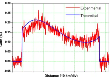
(6) > REPLACE THIS LINE WITH YOUR PAPER IDENTIFICATION NUMBER (DOUBLE-CLICK HERE TO EDIT) <. predicted by our model. We can see that the theoretical result provides a good fit to the experimental one, the disagreement coming mainly from the variation in the Brillouin shift along the fiber (our model assumes the Brillouin gain constant and maximum all over the fiber). The gain decreases exponentially with the distance as the only consequence of the linear attenuation. This means that, at the far end of the fiber, the gain to be measured is of the order of 0.02%, which is extremely small and gives a large uncertainty in the Brillouin shift determination. 0.40 0.35 0.30. Experimental Theoretical. 0.25. Gain (%). Raman-assisted configurations that have been introduced before. The measurements have been performed using a Brillouin pump pulse-width of 20 ns (2 meter spatial resolution) over 75 kilometers (result of splicing three spools of 25 km) of single mode fiber (SMF). The fiber has an effective area of 70 µm2. The Brillouin frequency shift is approximately the same in the fibers of the three spools (around 10.65 GHz), since they have been drawn consecutively from the same preform. This has been deliberately chosen to work in the most critical conditions (maximum Brillouin pump depletion). For comparison, we also show the trace in absence of Raman amplification. To achieve a clean trace, one has to average many acquisitions, so as to reduce the noise. In the conventional BOTDA setup, the noise comes from several sources, mainly: the Rayleigh backscatter of the pump, SBS caused by the imperfect extinction ratio of the Brillouin pump pulse and the erbium amplifier. In the cases of Raman assistance, the Raman laser additionally introduces a strong relative intensity noise that is transferred to the trace. In the traces shown next, the number of averages is 1000 in all the cases, to make a fair noise comparison in all the configurations. This way, we can see not only the gain contrast improvement over the fiber achieved through Raman amplification but also the issues related to the decrease in signal to noise ratio. Thus, we make the measurements in the same conditions always so as to show that even with this extra noise, we achieve better measurement results due to the contrast increase. To correctly determine the Brillouin frequency shift, depletion of the Brillouin pump due to Brillouin power transfer must be made negligible, since we would otherwise create a frequency dependent distortion in the trace that would render the measurement incorrect. Therefore, relatively low Brillouin pump powers and gain values (normally 1-2%) must be preferably chosen. Thus, the amount of Raman amplification that we need to generate is relatively low, just as much as needed to achieve propagation close to transparency. More amplification would deteriorate the performance since a strong increase in the Brillouin gain would lead to pump depletion and incorrect measurements. This optimum value of Raman pumping is always around 300 mW on each side (total power around 600 mW in the case of bi-directional amplification). Additionally, for each configuration we have to search for the optimum Brillouin pump and probe powers so as to avoid pump depletion and maximize the measurement range. The probe power is set high enough to ensure that the measured signal is as high as possible without saturating the amplifier. The Brillouin pump is set as high as possible but still trying to avoid depletion. Thus, we show the optimum measurement conditions found with these criteria for all the configurations. When the BOTDA operates without Raman amplification, the optimum values found are 4.7 mW for the peak power of the Brillouin pump pulse, and 5.2 µW for the probe power. The results obtained at a pump-probe frequency shift of 10.65 GHz are shown in Fig. 4, together with the theoretical curve. 6. 0.20 0.15 0.10 0.05 0.00. Distance (10 km/div). Fig. 4. Theoretical and experimental gain trace obtained with the BOTDA without Raman amplification. The peak power of the Brillouin pump pulse is 4.7 mW and the probe wave power is 5.2 µW. The measurement has been made at the average Brillouin shift of the fiber: 10.650 GHz. In the bi-directional Raman pumping configuration, the optimal pump peak power is 3.2 mW and the probe wave power is adjusted to 0.4 µW. Note that both pump and probe powers have been significantly reduced so as to avoid Brillouin gain saturation. This measurement has been made using a Raman pump power of 610 mW (305 mW on each side) which is basically enough to ensure transparency of the fiber on an end-to-end perspective. The results are presented in Fig. 5. As shown, the gain distribution is quite flat in the bidirectional configuration. This is a good advantage of this configuration, since the dynamic range of the measurement system does not need to accommodate large variations (this is not the case of the previous configuration, for instance). All over the fiber, the gain is well over 0.1%, which is still comfortable to perform a measurement. The biggest disadvantage is that this configuration also exhibits larger noise than the previous one, as it can be seen in the figure. This noise is caused by Relative Intensity Noise (RIN) transfer from the Raman pumps (the RIN of the RFL is -110 dBc/Hz). We believe that this RIN issue can be much improved with semiconductor pumps, which usually exhibit much better RIN values..

(7) > REPLACE THIS LINE WITH YOUR PAPER IDENTIFICATION NUMBER (DOUBLE-CLICK HERE TO EDIT) < 0.200. 0.30 0.25. Experimental. 0.175. Experimental. Theoretical. 0.150. Theoretical. 0.125. Gain (%). 0.20. Gain (%). 7. 0.15 0.10. 0.100 0.075 0.050 0.025. 0.05. 0.000. 0.00. -0.025. Distance (10 km/div). Fig. 5. Theoretical and experimental gain trace obtained with the BOTDA and bi-directional Raman amplification. The peak power of the Brillouin pump pulse is 3.2 mW and the probe wave power is 0.4 µW. The total Raman pump power is 610 mW (305 mW on each side). The measurement has been made at the average Brillouin shift of the fiber: 10.650 GHz. For the co-propagating Raman pump configuration, the best results are obtained with the following settings: peak Brillouin pump power set to 1.9 mW, probe power set to 1.7 µW, and a Raman pump power of 355 mW. The gain trace obtained for these settings is shown in Fig. 6. Again, it must be stressed that the Brillouin pump power has been significantly reduced to avoid gain saturation. In this case the noise is smaller than in the previous case, but at the far end of the fiber the gain values to be measured are only slightly larger than in the case of no Raman pumping. Again, this is a strong drawback in this configuration, although as we will see, the Brillouin shift determination is still better than without the Raman pumping. For the counter-propagating configuration, the optimum performance is found when the peak Brillouin pump power is set to 18.8 mW and the probe wave power has been adjusted to 0.25 µW. The Raman pump power is 302 mW. Note that in this case the Brillouin pump power has been increased very significantly while the probe wave has been strongly reduced. This means that the gain contrast that we can obtain at the beginning of the fiber is much larger even than the one obtained in the non-pumped case while the contrast in the far end of the fiber is in the order of 0.1%, which is still comfortable to measure. Still, the noise increase is evident but, as we will see, there is also a good improvement in Brillouin shift determination.. Distance (10 km/div) Fig. 6. Theoretical and experimental gain traces obtained for the copropagating configuration. The peak Brillouin pump pulse power is 1.9 mW and the probe wave power is 1.7 µW. The experimental Raman pump power is 355 mW. The measurement has been made at the average Brillouin shift of the fiber: 10.650 GHz 1.4 1.2 1.0. Experimental Theoretical. 0.8. Gain (%). -0.05. 0.6 0.4 0.2 0.0. Distance (10 km/div) Fig. 7. Theoretical and experimental measures for the counter-propagating configuration with Brillouin pump power of 18.8 mW and probe wave power of 0.25 µW. The experimental Raman pump power is 302 mW. The measurement has been made at the average Brillouin shift of the fiber: 10.650 GHz. As it is possible to observe, the theoretical results fit quite well to the experimental measurements in all the configurations, confirming the validity of the assumptions used to solve the model. We remember that the used model is the simplest one. It assumed that the non analytic term at equation 12 is zero. In Fig. 8 we compare all the experimental results shown above in a single graph. As we can see, the counterpropagating configuration shows a good improvement in contrast with respect to all the other configurations..

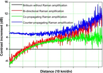
(8) > REPLACE THIS LINE WITH YOUR PAPER IDENTIFICATION NUMBER (DOUBLE-CLICK HERE TO EDIT) < 1.4. Brillouin without Raman amplification 1.2. Bi-directional Raman amplification. 1.0. Co-propagating Raman amplification. Gain (%). 0.8. Counter-propagating Raman amplification. 0.6 0.4 0.2 0.0. Distance (10 km/div) Fig. 8. Comparison of the optimum gain traces obtained in all the configurations (measurement conditions shown in the text and previous figures). We can see that the best gain contrast is obtained for the counterpropagating configuration, which shows an improvement in contrast all over the trace with respect to all the rest of the cases.. similar trend can also be observed if one evaluates the deviation between the measurements performed in all the configurations. Fig 11 shows the difference between the average Brillouin shift, and the actual shift measured with each configuration. As we can see, this deviation can reach ±15 MHz towards the far end of the fiber in the case of the conventional BOTDA system while in all the cases of Raman assistance this deviation remains below ±4 MHz. The poor results of the plain BOTDA configuration are due to the low gain contrast at the far end of the fiber. In the case of counterpropagating Raman pump, the deviation between measurements is below ±3 MHz. This means that the gain enhancement given by Raman is very helpful to reduce the uncertainty of the measurement, especially in the case of counter-propagating Raman assistance. 10.665 Brillouin without Raman amplification. 16. Frequency shift (GHz). 10.660. Fig. 9 shows the contrast enhancement achieved in all the configurations with respect to the case without amplification. As mentioned before, the largest contrast enhancement comes in the case of counter-propagating Raman amplification. Anyway, on average, the contrast of the traces is improved in all Raman configurations. The loss in contrast at the input end in the co-propagating and bi-directional configurations is due to the reduction in pump power that has been introduced to avoid pump depletion. It is also noticeable that the contrast enhancement in the co-propagating configuration saturates towards the far end of the fiber, while it increases towards the far end in the other two.. 10.645. 10.640. 10.635. Distance (10 km/div) Fig. 10. Brillouin Frequency shift in the same conditions that the experimental results presented before for all configurations. These experimental results have been obtained by fitting a frequency sweep of the probe wave signal.. 14 Brillouin without Raman amplification. Counter-propagating Raman amplification. 0. -4. Distance (10 km/div) Fig. 9. Contrast increment obtained in each of the configurations compared in Fig. 8 with respect to the non-assisted BOTDA case (black line).. It is important now to observe the improvements obtained in the determination of the Brillouin shift. Fig. 10 shows the Brillouin shift determined with the gain traces shown above. The variations in the Brillouin shift of the fibers are most probably due to some longitudinal variation in the construction parameters of the fiber (probably the GeO2 doping). As we can see, in all the configurations, the variance of the determined νB grows towards the end of the fiber. A. |νmeas - νave| (MHz). Contrast increment (dB). 16. Bi-directional Raman amplification. 4. Counter-propagating Raman amplification. 10.650. Co-propagating Raman amplification. 8. Bi-directional Raman amplification Co-propagating Raman amplification. 10.655. Brillouin without Raman amplification. 12. 8. 12. Bi-directional Raman amplification. 10. Co-propagating Raman amplification Counter-propagating Raman amplification. 8 6 4 2 0. Distance (10 km/div) Fig. 11. Absolute value of the difference between the average Brillouin Frequency shift in all Raman configurations and Brillouin frequency shift of the traces that have been shown at Fig. 9.. All the values of Brillouin shift represented in Fig. 10 have been obtained by fitting the experimental frequency sweep for each point to a Gaussian function and computing the position of the maximum gain. We have selected a Gaussian fit because the pulse is short enough to result in a broadened effective gain through convolution with the pump spectrum..

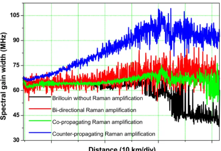
(9) > REPLACE THIS LINE WITH YOUR PAPER IDENTIFICATION NUMBER (DOUBLE-CLICK HERE TO EDIT) <. δω(t ) = −γL.  τ2 ∂ 2 τ A = 2γP0 L 2 exp − 2 ∂t τ0  τ0.    . (14). (this value, obtained using equation 15, is a lower bound since the losses for the Brillouin pump are smaller than the actual fiber loss due to the Raman gain) the calculated broadening in the pump exceeds ± 10 MHz in the maximum. This spectral broadening (20 MHz total) is more or less well correlated with the growth in the spectral width of the interaction that can be observed at Fig. 12 for the counter-propagating configuration. In the rest of configurations the pump power is lower, so the SPM broadening remains approximately below ± 3 MHz in the worst case. We can see more directly the impact of the SPM in the Brillouin gain spectrum by observing the frequency sweeps for a given position close to the fiber end. To do this, we measure the Brillouin gain spectra at 60 km for all the configurations tested. The results are shown in Fig. 13, together with the gain spectra measured at the beginning of the fiber for all the configurations. To improve the visualization, we average the acquisitions 4000 times in this case. We can see that at the beginning of the fiber, the spectrum maps well the non-assisted spectrum in all the cases. However, for the spectra acquired towards the 60th km, the measurements with the counter-propagating configuration show slightly higher wings. Since there is good contrast in this case, this fact does not perturb too much the correct determination of the Brillouin shift. However this is something to take into account when envisaging longer working distances. 105. Spectral gain width (MHz). This is manifested with the estimated width, that is much broader than the Brillouin natural line-width (35 MHz). The width in our graphs is measured as full-width at half maximum (FWHM). It is also interesting to have a look at the evolution of the spectral width of the Brillouin gain with the distance. The Brillouin gain spectral width obtained with this fitting procedure is shown in Fig. 12. In this figure we can observe that the plain BOTDA setup yields a spectral width of the interaction all over the fiber of approximately 65 MHz (the results beyond the 50th kilometer in this configuration are not very significant considering the uncertainty in the Brillouin shift estimated above). This Brillouin gain bandwidth can be explained through the convolution principle as follows. The pump pulse can be considered as a transform-limited pulse. Thus, the spectral width is the width of the spectrum of a 20 ns square pulse, this is approximately 25-30 MHz. Convolved with a 35 MHz gain curve, this gives approximately the 60-65 MHz of linewidth observed in the experiment. While in the bi-directional and co-propagating configurations the spectral gain width is preserved all over the fiber, in the counter-propagating configuration the width grows monotonically towards the end of the fiber, saturating at a value of 100 MHz beyond the 50th kilometer. This is probably due to the fact that in the counter-propagating configuration, the Brillouin pump power is the highest of all the configurations. This leads to some spectral broadening of the pump through self-phase modulation (SPM), which manifests as a growth in the measured Brillouin gain bandwidth. SPM accounts for self-induced phase and frequency changes that are produced by an intense optical pulse as it travels through an optical fiber. The intensity-dependent refractive index leads the pulse to modulate its own optical phase according to its intense profile. The varying phase shift across the pulse can also be viewed as a frequency chirp, that leads to spectral broadening. We can quantify the spectral broadening using the NLSE equation [17]. Neglecting fiber dispersion and losses and imposing Gaussian pulses at the fiber input |A(τ)|2=P0exp(-τ2/τ02), the instantaneous frequency change caused by SPM is given by (14).. 9. 90. 75. 60 Brillouin without Raman amplification Bi-directional Raman amplification. 45. Co-propagating Raman amplification Counter-propagating Raman amplification. 30. Distance (10 km/div) Fig. 12. Brillouin gain spectral width of the three Raman-assisted configurations and the traditional Brillouin sensor. This experimental result has been obtained fitting the frequency sweep at each distance.. 1,2. 1,2. Using equation (14), we can estimate a lower bound of the frequency chirp imposed on the Brillouin pump pulse for the counter-propagating Raman configuration. Using the values of pump power (P0) of 18 mW, γ of 2 W-1·km-1 and Leff of 22 km. 1,0 0,8. Normalized gain. 0,8. Normalized gain. where γ is the non-linear coefficient, P0 is the pump power, L is the fiber length, A(τ) is the Gaussian pulse shape and τ0 is the pulse width. If we consider the losses in the fiber, L should be replaced by Leff, which is calculated by (15). L 1 − exp(− αz ) Leff = ∫ exp(− αz )dz = (15) 0 α. 1,0. 0,6 0,4 0,2. Non-assisted Bi-directional Co-propagating Counter-propagating. 0,0 -0,2 10,60. 10,65. Frequency (GHz). (a). 0,6 0,4 0,2. Non-assisted Bi-directional Co-propagating Counter-propagating. 0,0. 10,70. -0,2 10,55. 10,60. 10,65. 10,70. Frequency (GHz). (b). Fig. 13. Normalized Brillouin gain spectra measured at the input of the fiber with all the configurations (a) and after 60 km (b). The increase in the wings of the spectrum in the counter-propagating case is attributed to self-phase modulation..

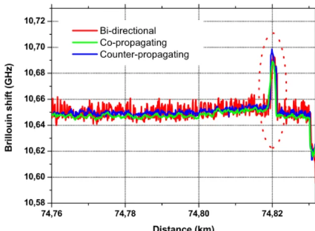
(10) > REPLACE THIS LINE WITH YOUR PAPER IDENTIFICATION NUMBER (DOUBLE-CLICK HERE TO EDIT) <. VI. HOT SPOT DETECTION TESTS. 10,72. To verify the correct operation of the setup as a sensor we made some hot spot detection experiments. We inserted ~2 meters of the sensing fiber just before the far end (74.82 km) in a water bath with controlled temperature (around 50ºC, with 5ºC hysteresis). This acts as a hot spot with respect to the lab temperature, which is kept around 20ºC. The frequency sweep was done in the conditions of the previous section for all the measurement configurations, except for the number of averages, which was increased in all cases up to 16000 averages. The tests where done in all the Raman-assisted configurations. Results of a sample sweep (counterpropagating configuration) are shown in Figure 14.. 10.7. Brillouin shift (GHz). 10,68 10,66 10,64 10,62 10,60 10,58 74,76. 74,78. 74,80. 74,82. Distance (km). 10.68. VII. CONCLUSION. 10.66. 10.64. 10.62 74.76. Bi-directional Co-propagating Counter-propagating. Fig. 15. Brillouin shift determination around the hot-spot location (74.82 km) Measurement conditions are the ones shown in the previous section for all the configurations except for the number of averages per frequency, which was increased to 16000.. 10.72. Frequency (GHz). 10,70. 10. 74.78. 74.8 74.82 Distance (km). 74.84. 74.86. Fig. 14. Traces obtained close to the hot-spot location (74.82 km) for a pumpprobe frequency sweep between 10.61 GHz and 10.72 GHz. Measurement conditions are shown in the caption of Fig 7.. Figure 15 shows the measured Brillouin shift as a function of the position around the hot spot for all the Raman-assisted configurations. We can see that all the configurations correctly determine the location of the hot spot and also give a good estimation of the Brillouin shift change in that location. All the configurations give a Brillouin shift change in the hotspot location of approximately 40 MHz. Considering the sensitivity of the Brillouin shift to temperature (1.3 MHz/ºC), this gives a temperature change of roughly 30ºC, which agrees well with the expected temperature change. Out of the hot spot, the co- and counter-propagating Raman configurations agree very well, while in the hot-spot they seem to show a small disagreement of 7 MHz (slightly more than 5ºC). We believe that this is probably more due to the hysteresis in the temperature controller of the bath rather than the performance of the actual measurement setup. The bi-directional configuration, however, shows a much larger noise all over the trace, which is caused by the RIN transfer from the Raman pump.. We have presented a Raman-assisted distributed sensor based on stimulated Brillouin scattering for sensing temperature and strain. This experimental setup allows us to monitor up to 75 km of optical fiber with a resolution of 2 meters, with marked contrast improvement at long distances due to the effect of distributed amplification. We have tested three different Raman pumping configurations: copropagating, counter-propagating and bi-directional propagation (referring to the direction of propagation of the Brillouin pump pulse). The best results in terms of contrast are obtained for the counter-propagating and bi-directional schemes (specially the first one). The bi-directional configuration allows achieving a quasi-constant gain distribution, which is interesting because the dynamic range in detection does not need to be very broad (unlike the other configurations). The results also highlight the importance of the RIN in the Raman pump. The experimental results allow us to envisage the possibility of extending the monitored distance up to 100 km in a near future, keeping the same spatial resolution. ACKNOWLEDGMENT We acknowledge M. V. Andrés and J. L. Cruz for providing the Bragg gratings used in our experimental setup and the collaborative environment of the European COST Action 299 "FIDES". REFERENCES [1] [2]. T. Horiguchi and M. Tateda, “Optical-fiber-attenuation investigation using stimulated Brillouin scattering between a pulse and a continuous wave”. Opt. Lett., vol. 14, no. 8, pp. 408-410, 1989. T. Horiguchi, T. Kurashima and M. Tateda, “A technique to measure distributed strain in optical fibers”. IEEE Photonics Technology Letters, vol. 2, issue 5, pp. 352-354, 1990..

(11) > REPLACE THIS LINE WITH YOUR PAPER IDENTIFICATION NUMBER (DOUBLE-CLICK HERE TO EDIT) < [3] [4] [5] [6]. [7] [8] [9] [10]. [11] [12]. [13]. [14]. [15] [16]. [17] [18] [19]. [20]. T. Horiguchi, T. Kurashima and M. Tateda, “Tensile strain dependence of Brillouin frequency shift in silica optical fibers”. IEEE Photon. Tech. Lett. PTL-1, 107-108, 1989. X. Bao, F. Ravet and L. Zou, “Distributed Brillouin sensor based on Brillouin scattering for structural health monitoring”. Fiber Optic Sens Syst 20(6):9–11, 2005. X. Bao, J. Webb and D. A. Jackson, “32-km distributed temperature sensor based on Brillouin loss in an optical fiber”. Optics Letters, Vol. 18, Issue 18, pp. 1561-1563, 1993. M. Niklès, L. Thévenaz and P. A. Robert, “Simple distributed temperature sensor based on Brillouin gain spectrum analysis”. Proc. SPIE Vol. 2360, p. 138-141, Tenth International Conference on Optical Fibre Sensors, 1994. M. Niklès, L. Thévenaz and P. A. Robert, “Simple distributed fiber sensor based on Brillouin gain spectrum analysis”. Optics Letters, Vol. 21, Issue 10, pp. 758-760, 1996. M. Niklès, L. Thévenaz and P. A. Robert, “Brillouin gain spectrum characterization in single-mode optical fibers”. Journal of Lightwave Technology, Vol. 15, NO. 10, 1842-1851, 1997. J. Smith, A. Brown, M. DeMerchant and X. Bao, “Simultaneous distributed strain and temperature measurement”. Applied Optics, Vol. 38, Issue 25, pp. 5372-5377. 1999. H. Naruse, M. Tateda, H. Ohno and A. Shimada, “Dependence of the Brillouin gain spectrum on linear strain distribution for optical timedomain reflectometer-type strain sensors”. Applied Optics, Vol. 41, Issue 34, pp. 7212-7217, 2002. M. Niklès, “Fibre optic distributed scattering sensing system: Perspectives and challenges for high performance applications”. Third European Workshop on Optical Fiber Sensors, 66190D, Italy, 2007. A. W. Brown, M. D. DeMerchant, X. Bao and T. W. Bremner, “Spatial resolution enhancement of a Brillouin-distributed sensor using a novel signal processing method”. Journal of Lightwave Technology, Vol. 17, Issue 7, pp. 1179-1183, 1999. Y. T. Cho, M. N. Alahbabi, M. J. Gunning and T. P. Newson, “50-km single-ended spontaneous-Brillouin-based distributed-temperature sensor exploiting pulsed Raman amplification”. Optics Letters, Vol. 28, Issue 18, pp. 1651-1653, 2003. Y. T. Cho, M. N. Alahbabi, M. J. Gunning and T. P. Newson, “Enhanced performance of long range Brillouin intensity based temperature sensors using remote Raman amplification”. Measurement Science & Technology, 2004. 15(8): p. 1548-1552, 2004. M. N. Alahbabi , Y. T. Cho and T. P. Newson, “100-km distributed temperature sensor based on coherent detection of spontaneous Brillouin backscatter”. Meas. Sci. Technol. 15, 1544–1547, 2004. M. N. Alahbabi, Y. T. Cho and T. P. Newson, “150-km-range distributed temperature sensor based on coherent detection of spontaneous Brillouin backscatter and in-line Raman amplification”. JOSA B, Vol. 22, Issue 6, pp. 1321-1324, 2005. G. P. Agrawal, Nonlinear Fiber Optics, 4th ed. Academic Press, San Diego, 2007. Chap. 9. K. Brown, A. W. Brown and B. Colpitts, “Characterization of optical fibers for optimization of a Brillouin scattering based fiber optic sensor”. Opt. Fiber Technol., vol. 11, no. 2, pp. 131-145, Apr, 2005. T. Horiguchi and M. Tateda, “BOTDA-Nondestructive measurement of single-mode optical fiber attenuation characteristics using Brillouin interaction: Theory”. J. Lightwave Technol., vol. LT-7, no. 8, pp. 11701176, 1989. A. Carrasco-Sanz, F. Rodriguez-Barrios, P. Corredera, S. Martin-Lopez, M. Gonzalez-Herraez, and M. L. Hernanz, “An integrating sphere radiometer as a solution for high power calibrations in fiber optics,” Metrologia, vol. 43, no. 2, pp. 145–150, 2006.. Félix Rodríguez-Barrios was born in Zamora, Spain in 1983. He received the telecommunications degree from the Polytechnic University of Madrid, Madrid, Spain, in 2006 and the Master degree in Advanced Electronics Systems from Carlos III University of Madrid, Leganés, Spain, in 2008. Since 2007, he has been working towards the Ph.D. degree at the Institute of Applied Physics, Spanish Council for Research, Madrid, Spain. His current research interests include nonlinear fiber optics and fiber optic sensors.. 11. Sonia Martín López received the Ph.D degree from the Universidad Complutense de Madrid in May 2006. The topic of her doctoral dissertation was on experimental and theoretical understanding of continuous-wave pumped supercontinuum generation in optical fibers. She had a long stay in the Nanophotonics and Metrology Laboratory, Ecole Polytechnique Federale de Lausanne, Switzerland. She is currently engaged as a post-doctoral researcher in the Applied Physics Institute at the Spanish Council for Research. She is author or co-author of 30 papers in international refereed journals and conference contribution. Her current research interests include nonlinear fiber optics. Ana Carrrasco Sanz received the M.Eng. degree in electronic engineering (2002), B.Sc. degree in physics (2003) and Ph.D degree (2007) from the University of Granada. The topic of her doctoral dissertation was on the synthesis of standard frequencies for WDM system calibration for optical communications. The work was carried out in the Applied Physics Institute at the Spanish Council for Research. She had a stay in the Danish Fundamental Metrology, Denmark and in EXFO Electro-Optical Engineering, Canada. In October 2008, she was appointed Assistant Professor in the Department of Optics, University of Granada, Spain, where she is currently engaged. Her current research interests include nonlinear interaction in optical fibers and semiconductor optical amplifiers. Juan Diego Ania-Castañón (MSc’96-PhD’00) was born in Oviedo (Spain) in 1973. He obtained his MSc in Physics from Universidad Complutense de Madrid (Spain), and his PhD in Theoretical Physics from Universidad de Oviedo and Instituto de Estructura de la Materia, CSIC, Madrid (Spain). In 2001 he joined the Photonics Research Group at Aston University, in Birmingham (United Kingdom), first as a Contract Research Fellow and then as an EPSRC Advanced Research Fellow from 2004. In 2007 he took an appointment as Tenured Scientist at Instituto de Óptica, CSIC, Madrid (Spain). His main research interests include the study of nonlinear dynamics in optical systems and the exploitation of nonlinear effects in optical fiber. Pedro Corredera received the B.Sc. and Ph.D. degrees in physics from the University of Salamanca, Salamanca, Spain, in 1985 and 1989, respectively. In 1996, he joined the Institute of Applied Physics, CSIC, where he is currently a Research Manager of the Fibre Optics Laboratory. His current research interests include fiber-optic measurements, optical fiber sensors, nonlinear fiber optics, and IR radiometry and detection. Luc Thévenaz (M’02) received the M.Sc. degree in astrophysics from the Observatory of Geneva, Geneva, Switzerland, in 1982 and the Ph.D. degree in physics from the University of Geneva, Geneva, Switzerland, in 1988, where he developed his field of expertise, namely, fiber optics. In 1988, he joined the Swiss Federal Institute of Technology of Lausanne (EPFL), Switzerland. In 1991, he visited the PUC University, Rio de Janeiro, Brazil, and Stanford University, Stanford, CA, where he participated in the development of a Brillouin laser gyroscope. In 1998 and 1999, he stayed at the Korea Advanced Institute of Science and Technology (KAIST), Daejon, South Korea, where he worked on fiber laser current sensors. Currently, he leads a research group at the EPFL that is involved in photonics, in particular, fiber optics and optical sensing. Research topics include electrical current fiber sensors, Brillouin-scattering fiber sensors, fiber nonlinearities measurement techniques, and laser-diode spectroscopy of gases. Miguel González-Herráez received the M.Eng. and D.Eng. degrees from the Polytechnic University of Madrid, Madrid, Spain, in 2000 and 2004, respectively. While working towards the D.Eng. degree, he worked first as a Research Assistant and then a Postdoctoral Fellow in the Applied Physics Institute at the Spanish Council for Research, Madrid, Spain, and had several long stays in the Nanophotonics and Metrology Laboratory, Ecole Polytechnique Federale de Lausanne, Switzerland. In October 2004, he was appointed Assistant Professor in the Department of Electronics, University of Alcalá, Madrid, Spain, where he was promoted to Associate Professor in June 2006. He is the author or coauthor of over 100 papers in international refereed journals and conference contributions and has given several invited talks at international conferences. His research interests cover the wide field of nonlinear interactions in optical fibers..

(12)