J. Phys. D: Appl. Phys.38(2005) 1282–1291 doi:10.1088/0022-3727/38/8/028
The effect of heat transfer laws and
thermal conductances on the local
stability of an endoreversible heat engine
L Guzm´an-Vargas
1,3, I Reyes-Ram´ırez
1and N S´anchez
2 1Unidad Profesional Interdisciplinaria en Ingenier´ıa y Tecnolog´ıas Avanzadas, Instituto Polit´ecnico Nacional, Av. IPN No. 2580, L. Ticom´an, M´exico D.F. 07340, M´exico 2Departamento de F´ısica, Escuela Superior de F´ısica y Matem´aticas, Instituto Polit´ecnico Nacional, Edif. No. 9 U.P. Zacatenco, M´exico D.F. 07738, M´exicoE-mail: [email protected]
Received 2 September 2004, in final form 18 January 2005 Published 1 April 2005
Online atstacks.iop.org/JPhysD/38/1282
Abstract
In a recent paper (Santill´anet al 2001J. Phys. D: Appl. Phys.342068–72) the local stability of a Curzon–Ahlborn–Novikov (CAN) engine with equal conductances in the coupling with thermal baths was analysed. In this work, we present a local stability analysis of an endoreversible engine operating at maximum power output, for common heat transfer laws, and for different heat conductancesαandβ, in the isothermal couplings of the working substance with the thermal sourcesT1andT2(T1> T2). We find that the
relaxation times, in the cases analysed here, are a function ofα,β, the heat capacityC,T1andT2. Besides, the eigendirections in a phase portrait
are also functions ofτ =T1/T2and the ratioβ/α. From these findings,
phase portraits for the trajectories after a small perturbation over the steady-state values of internal temperatures are presented, for some significant situations. Finally, we discuss the local stability and energetic properties of the endoreversible CAN heat engine.
(Some figures in this article are in colour only in the electronic version)
1. Introduction
In recent years, finite time models for the operation of thermal engines have attracted the attention of researchers following
very different approaches [1–3]. This new discipline,
called finite-time thermodynamics (FTT) has emerged as an extension of traditional equilibrium thermodynamics and is used to obtain more realistic limits for the performance of real engine models.
FTT started with a paper published by Curzon and
Ahlborn in 1975 [4]. In this paper an endoreversible
Curzon–Alhborn–Novikov (CAN) engine was introduced. This model takes into account irreversibilities due to the coupling between the working fluid and the thermal reservoirs, and through thermal conductors governed by the linear Newton
3 Author to whom any correspondence should be addressed. Present address: Department of Chemical and Biological Engineering, Northwestern University, Evanston, IL 60202, USA.
heat transfer law. Furthermore, in real engines not all heat transfer obeys this law and it is consequently essential to study the effect of different transfer laws; several authors
have studied this issue [5–8]. Also, it is worth noting
that real thermal engines are built from different materials. In more realistic models, it is then natural to assume different conductances at hot and cold branches of the thermal cycle.
Most of the studies of FTT have focused on steady-state energetic properties. However, all thermal engines work with many cycles per unit of time and, however similar may be, they are never identical, that is, there exists intrinsic cyclic
variability (CV) in any sequence of cycles. For example,
the stability of the system’s steady state. This study may allow us to guarantee proper dynamical behaviour of a system like stability and small relaxation times, or to warn about possible failure in the performance of a thermal engine.
In a recent work [10], Santill´an et al studied the local
stability of a CAN engine operating at maximum power, with equal conductances in both isothermal branches of the cycle. In this work, following the direction suggested by the findings
of Santill´anet al [10] and taking into account all the facts
discussed above, we analyse the stability of a endoreversible engine with several heat transfer laws and with different heat conductances at the isothermal branches. The paper is
organized as follows. In section 2, we describe the local
stability analysis method applied to a two-dimensional system. In section 3, a brief description of an endoreversible engine is presented. In section 4, the local stability analysis of a CAN engine with different heat transfer laws is described. Finally, in section 5, we discuss our results from a thermodynamic perspective.
2. Linearization and stability analysis
In this section, we present a brief description of both the linearization technique for two-dimensional dynamical systems, and fixed point local stability analysis [11]. Consider the dynamical system
dx
dt =f (x, y) (1)
and
dy
dt =g(x, y). (2)
Let (x,¯ y)¯ be a fixed point such that f (x,¯ y)¯ = 0 and
g(x,¯ y)¯ =0. Consider a small perturbation around this fixed
point and write x = ¯x +δx and y = ¯y +δy, where δx
andδy are small disturbances from the corresponding fixed
point values. By substituting into equations (1) and (2),
expandingf (x¯+δx,y¯+δy)andg(x¯+δx,y¯+δy)in a Taylor
series, and using the fact thatδx andδy are small to neglect
quadratic terms, the following equations are obtained for the perturbations:
dδx
dt
dδy
dt
=
fx fy
gx gy
δx δy
, (3)
wherefx =∂f /∂x|x,¯y;¯ fy =∂f /∂y|x,¯y;¯ gx =∂g/∂x|x,¯y¯ and
gy=∂g/∂y|x,¯y¯. Equation (3) is a linear system of differential equations. Thus, we assume that the general solution of the system is of the form
δr=eλtu, (4) with δr = (δx, δy) andu = (ux, uy). Substitution of the
solutionδrinto equation (3) yields the following eigenvalue
equation:
Aδr=λδr, (5)
whereAis the matrix given by the first term on the right-hand
side of equation (3). The eigenvalues of this equation are the roots of the characteristic equation
|A−λI| =0 (6)
or
(fx−λ)(gy−λ)−gxfy =0. (7)
Ifλ1andλ2are solutions of equation (7), the general solution
of the system is
δr=c1eλ1tu1+c2eλ2tu2, (8)
where c1 andc2 are arbitrary constants and u1 and u2 are
the eigenvectors corresponding to λ1 and λ2, respectively.
To determineu1andu2 we use equation (5) again for each
eigenvalue. Information about the stability of the system can
be obtained from the values of the eigenvalues λ1 andλ2.
In general,λ1 andλ2are complex numbers. If bothλ1 and
λ2have negative real parts, the fixed point is stable. Moreover,
if both eigenvalues are real and negative, the perturbations decay exponentially. In this last case, it is possible to identify characteristic time scales for each eigendirection as
t1= 1
|λ1|
(9)
and
t2= 1
|λ2|
. (10)
3. The endoreversible engine
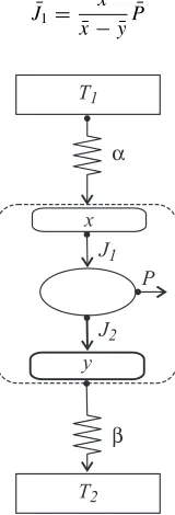
Consider the endoreversible engine depicted in figure 1. The
engine operates between temperaturesT1andT2, withT1> T2.
Heat flows irreversibly fromT1tox¯ and fromy¯toT2(T1 >
¯
x >y > T¯ 2). Here and in what follows, we use overbars to denote steady-state values. The endoreversibility hypothesis states that the system is internally reversible. That is, a Carnot
cycle operates between temperaturesx¯andy¯. This hypothesis
further implies that the heat flows can be expressed as [10]
¯
J1= ¯
x
¯
x− ¯yP¯ (11)
T1
T2 J2 x
y P
α
β
[image:2.595.381.461.478.713.2]J1
Figure 1.Typical representation of an endoreversible CAN engine. The cycle operates between temperaturesT1andT2withT1> T2. A Carnot cycle takes place between internal temperaturesxandy
and
¯
J2= ¯
y
¯
x− ¯yP ,¯ (12)
whereJ1andJ2are the heat flows fromx¯to the engine and from
the engine toy¯, andP¯ is the power output. For the present
study we consider heat transfer laws that in the steady-state take the general form
¯
J1=α(T1k− ¯x
k) (13)
and
¯
J2=β(y¯k−T2k), (14)
withαandβbeing the thermal conductances at the high- and
low-temperature branches of the cycle, respectively. From equations (11)–(14) and the definition of efficiency,
¯
η= P¯¯ J1
, (15)
it is possible to express temperaturesx¯andy¯as
¯
xk=T1k
(1− ¯η)+(β/α)τk
(1− ¯η)+(β/α)(1− ¯η)k (16) and
¯
yk=T2k(1− ¯η)τ
−k+β/α
(1− ¯η)1−k+β/α, (17)
withτ=T2/T1. From equations (16) and (17) it follows that
T1k= ¯xk
(1− ¯η)+(β/α)(1− ¯η)k
(1− ¯η)+(β/α)τk (18) and
T2k= ¯yk
(1− ¯η)1−k+β/α
(1− ¯η)τ−k+β/α. (19) Using the fact that the cycle is internally reversible with efficiency
¯
η=1−y¯
¯
x, (20)
equations (18) and (19) can be written as
T1k= ¯
xky¯+(β/α)xyk
¯
y+(β/α)xτ¯ k (21) and
T2k= x¯
ky¯+(β/α)xyk
¯
yτ−k+(β/α)x¯ . (22) From equations (13), (15) and (16) it is possible to express the power output as
¯
P =αβT1kη¯ (1− ¯η)
k−τk
α(1− ¯η)+β(1− ¯η)k. (23)
Finally, substitution of equations (18) and (20) into
equation (23) yields
¯
P (x,¯ y)¯ =αβ(x¯− ¯y)(y¯
k− ¯xkτk)
αy¯+βxτ¯ k . (24)
4. Local stability analysis of an endoreversible engine
In this section, following Santill´anet al [10], a system of
differential equations that provides information on the stability
of an endoreversible engine is constructed. Santill´an et al
developed a system of coupled differential equations to model the rate of change of intermediate temperatures. Assuming that
the temperaturesxandy correspond to macroscopic objects
with heat capacityC, the differential equations forxandyare
given by [10]
dx
dt =
1
C[α(T
k 1 −x
k)−J
1] (25)
and
dy
dt =
1
C[J2−β(y
k−Tk
2)], (26)
whereJ1 andJ2 are the heat flows from x to the working
substance and from the Carnot engine to y, respectively
(see figure 1). According to the endoreversibility hypothesis,
J1andJ2are related to the power output by
J1=
x
x−yP (27)
and
J2=
y
x−yP . (28)
Substitution of equations (27) and (28) into equations (25) and (26) leads to
dx
dt =
1
C α(T
k 1 −x
k)− x
x−yP (x, y)
(29)
and
dy
dt =
1
C y
x−yP (x, y)−β(y
k−Tk 2)
. (30)
4.1. Casek=1
Whenk=1, equations (13) and (14) become a Newton’s heat
transfer law. It is well known that in this case the efficiency that maximizes the power output is [4]
¯
ηCA=1− √
τ , (31) while the maximum power output is given by [6]
P = αβ α+βT1[1−
√
τ]2. (32) Equating equations (20) and (31) gives
τ =y¯
2
¯
x2. (33)
The steady-state valuesx¯andy¯, as functions ofT1andT2, in the
maximum-power regime can then be obtained by substituting
equation (31) andk=1 into equations (16) and (17). That is,
¯
x=T1
α+β√τ
0.2 0.4 0.6 0.8 1 τ
0 2 4 6 8 10 12
relaxation times (x
α
/C)
β/α= 1
β/α= 0.5
β/α= 0.3
β/α= 0.1 β/α
= 3
β/α= 5
β/α= 8
β/α= 10
t1
01 0.2 0.4 0.6 0.8
τ 0
0.5 1 1.5 2
relaxation times (x
α
/C)
0 0.05 0.1 0.15 0.2
τ 0
0.5 1
relaxation times (x
α
/C)
}
}
t2t1 t2
[image:4.595.63.539.79.253.2](a) (b)
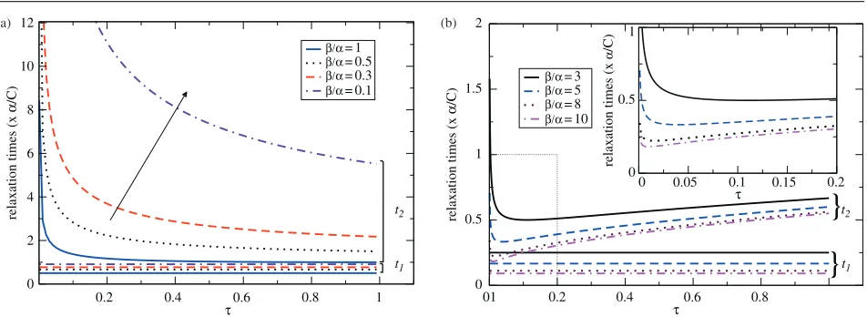
Figure 2.Plot of relaxation times versusτfor some values of the ratioβ/α, for a fixed value ofα. (a) For a given value of the ratio
β/α1,t1(k=1)is constant andt2(k=1)is a decreasing function ofτ. As the ratioβ/αdecreases both relaxation times increase. (b) Ifβ/α >1,
t2(k=1)shows a minimum at the special value√τ=α/β(see the inset). Similar plots can be obtained for a fixed value ofβand variation ofα.
and
¯
y=T1 √
τ
α+β√τ α+β
. (35)
Finally, substitution of equation (33) and k = 1 into
equation (24) allows the steady-state power output to be expressed as
¯
P (x,¯ y)¯ =αβ(x¯− ¯y)
2
αx¯+βy¯. (36)
The assumption of Santill´anet al[10] can be stated as follows:
out of the steady state but not too far away, the power of a CAN
engine depends onx andy in the same way that it depends
on x¯ andy¯ at the steady state (P (x,¯ y)¯ −→ P (x, y)). It
is then useful to perform the local stability analysis4. Using
this assumption, applicable only in the vicinity of the steady
state, it is possible to write the dynamic equations forxandy
(equations (29) and (30)) as
dx
dt =
1
C α(T1−x)−αβ
x(x−y) αx+βy
(37)
and
dy
dt =
1
C αβ
y(x−y)
αx+βy −β(y−T2)
. (38) To analyse the system stability near the steady state, we proceed following the steps described in section 2. Define,
f (x, y)= 1
C α(T1−x)−αβ
x(x−y) αx+βy
(39)
and
g(x, y)= 1 C αβ
y(x−y)
αx+βy −β(y−T2)
. (40) After solving the eigenvalue equation we get
λ(k1=1)= −α+β
C (41)
4 Consider a Taylor expansion of a real function in two variablesP (x, y)about the point(x,¯ y)¯:P (x, y)=P (x,¯ y)¯ +(x− ¯x)(∂P /∂x)+(y− ¯y)(∂P /∂y)+
O((x− ¯x)2, (y− ¯y)2)+· · ·. If the distances(x− ¯x)and(y− ¯y)are small
enough to be neglected, we can assume thatP (x, y)≈P (x,¯ y)¯.
and
λ(k2=1)= −2(α+β)αβ
√
τ
C(α+β√τ )2 . (42) The corresponding eigenvectors are given by
u(k1=1)=
1,−β
ατ
(43)
and
u(k2=1)=
1,α
β
. (44) It is easy to prove that both eigenvalues are real and negative. Therefore, the characteristic relaxation times can be defined as (see equations (9) and (10))
t1(k=1)= C
α+β (45)
and
t2(k=1)= C(α+β
√
τ )2
2(α+β)αβ√τ. (46)
As mentioned before, both eigenvalues are negative (λ(k1=1)< λ2(k=1)<0 ) for every 0< τ <1,β >0 andα >0. Thus, the steady state is stable because any perturbation would
decay exponentially. Whenα=βthe main results reported by
Santill´anet al [10] are recovered. In equation (45) we observe
a symmetric behaviour of the relaxation time for interchanges
ofα →β. Something similar would occur in equation (46)
except for the factor√τ in the numerator. In figures 2(a)
and 2(b) the relaxation times are plotted versusτfor different
values of the ratioβ/α, for a fixed value ofα >0. Ifβ/α1
(see figure (2a)), for a given value of the ratioβ/α,t1(k=1)is
constant andt2(k=1)is a decreasing function ofτ. The relaxation
times increase asβ/α decreases (figure 2(a)). In particular,
t2(k=1)grows in such a manner that whenβ/α→0,t2(k=1)→ ∞
and the stability is lost. In the opposite directionβ/α > 1,
t2(k=1)shows a minimum at the special value√τ =α/β (see
figure 2(b)). Asβ increases both relaxation times decrease.
Similar conclusions can be obtained if one assumes a fixed
100 200
300
0 100
200 300
β α
β α
100 200
300 0 100 200
300 k=1
τ= 1/2
k=1 τ= 1/2 0
0 0.1 0.2 (a)
(b)
relaxation time x 1/C
0 0 0.1 0.2
[image:5.595.63.297.78.265.2]relaxation time x 1/C
Figure 3.Plots of relaxation times against the conductancesαand
βwithτ=1
2for the casek=1. (a) The relaxation time (t (k=1)
1 )
diverges asαandβapproach the origin and decreases asαandβ
increase. (b) The relaxation time (t2(k=1)) diverges asα→0 for every value ofβand vice versa.
x y
fast eigendirection
λ1
slow eigendirecti on
λ2
α = β τ = 1/2
k =1
Figure 4.Qualitative phase portrait ofx(t )versusy(t )forβ=α
andτ=12. Both eigenvalues are negative and bothx(t )andy(t )
decay exponentially to the origin (steady-state valuesx,¯ y¯). In this case, 0< t1(k=1)< t2(k=1), witht2(k=1)/t1(k=1)≈2.06. The
corresponding eigenvectors can be described as the fast eigendirection (equation (43)) and the slow eigendirection
(equation (44)). In this plot the eigendirections areu(k1=1)=(1,−12)
andu(k2=1)=(1,1).
In figures 3(a) and 3(b) we plot the relaxation timest1(k=1)
andt2(k=1)againstαandβwith a fixed value ofτ = 12. The
relaxation time (t1(k=1)) is a decreasing function ofα andβ
(see figure 3(a)). If bothα→0 andβ→0,t1(k=1)diverges.
The second relaxation time (t2(k=1)) diverges as α→0 or
β→0. For large values ofα andβ, t2(k=1) is zero. From
these considerations, it follows that the stability of the system
declines in the limitsβ/α→0 andα/β→0.
From equations (45) and (46) we observe that 0< t1(k=1)< t2(k=1). Indeed, there is a stronger inequality
t2(k=1) 2t (k=1)
1 (the equality is valid for the special case
√
τ = α/β). In fact, the ratio t2(k=1)/t1(k=1) allows us to
compare the relaxation times along the eigendirections as a
function ofβ/αandτ. Thus, the corresponding eigenvectors
x y
τ =1/2 β/α =0.1
k =1
fast eigendirection slow eigendi
[image:5.595.303.537.81.248.2]rection
Figure 5.Qualitative phase portrait ofx(t )versusy(t )for
β/α=0.1 andτ=1
2. In this case,t (k=1) 2 /t
(k=1)
1 ≈8.1. The fast eigendirection (equation (43)) and the slow eigendirection (equation (44)) areu(k1=1)=(1,−0.05)andu(k2=1)=(1,10), respectively. Clearly, the fast eigendirection is almost parallel to the horizontal axis and something similar occurs with the slow eigendirection with the vertical axis. According to this, trajectories approach the origin (x,¯ y¯) tangent to the slow direction (y-axis) because the decaying ofx(t )is almost instantaneous.
can be described as a fast eigendirection (equation (43)) and
a slow eigendirection (equation (44)), respectively. Now,
it is possible to describe the phase space portrait with the
help of the eigendirections. In figure 4 we present the
phase portrait of the case β = α with τ = 0.5. In this
case, the trajectories approach the origin tangent to the slow
eigendirection. In backwards time (t→ −∞), the trajectories
are parallel to the fast eigendirection. In figure 5 we present
the case whenβ/α = 0.1, that is, the conductance at high
temperature is large. In this case, the fast eigendirection is close to the horizontal axis whereas the slow eigendirection is close to the vertical axis. For this reason, any perturbation
on x andy values tends to come back to the steady state,
decreasing thex temperature very fast in comparison to the
y temperature. A very different situation is observed when
β/α=10 (see figure 6), that is, close to the reversible release
of heat. In this case (figure 6), the fast eigendirection is close to the vertical axis and the slow eigendirection is almost parallel
to the horizontal axis; thus, under any perturbation onxandy,
the temperatureyreaches its steady-state value faster than the
temperaturex.
4.2. Casek= −1
Ifk = −1 then equations (13) and (14) represent the linear
phenomenological heat-transfer law of irreversible
thermody-namics [7, 8]. Now,αandβare negatives. The efficiency that
maximizes the power output in this case is given by [12]
¯
η(k=−1)=
1 +β/α−√1 +β/αβ/α+τ2
1 +τ . (47)
The maximum power output is given by [12]
P(k=−1)=
α
2T2
β α+τ−
1 +β
α
β α +τ
2
[image:5.595.62.291.341.504.2]k =1
x y
slow eigendirection
fast eigendire
ction
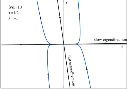
[image:6.595.291.537.84.333.2]β/α =10 τ=1/2
Figure 6.Qualitative phase portrait ofx(t )versusy(t )for
β/α=10 andτ=12. Now,t2(k=1)/t1(k=1)≈4.6. The fast eigendirection (equation (43)) and the slow eigendirection (equation (44)) areu(k1=1)=(1,−5)andu(k2=1)=(1,0.1), respectively. In this case, we have the opposite situation to that in figure (5); that is, the fast eigendirection is almost parallel to the vertical axis and the slow eigendirection to the horizontal axis. Now, trajectories approach the origin (x,¯ y¯) tangent to the slow direction (x-axis) because the decaying ofy(t )is almost instantaneous.
Equating equations (20) and (47) and solving forτwe obtain
τ = αy¯
2+ 2βxy−βx¯2
βx¯2+ 2αxy−αy¯2. (49)
The steady-state valuesx¯andy¯as a function ofT1andT2in
the maximum-power regime can be obtained by substituting
equation (47) andk= −1 into equations (16) and (17):
¯
x= 2T2
√
1 +β/α
τ√1 +β/α+β/α+τ2 (50) and
¯
y= 2T2
√
1 +β/α
√
1 +β/α+β/α+τ2. (51)
By substituting equation (49) andk= −1 into equation (24), it
is possible to write the steady-state power output as a function
ofx¯andy¯; that is,
¯
P(k=−1)(x,¯ y)¯ = −α
(x¯− ¯y)2
xy(x¯+(α/β)y)¯ . (52)
Using, again, the assumption that the power output of an
endoreversible engine, close to the steady state, hasxandy
dependences similar in form to the power in the steady-state
conditions (equation (52)), the dynamical equations forxand
y(equations (29) and (30)) are
dx
dt =
1 C α 1 T1 −1 x
+α (x−y)
y(x+(α/β)y
, (53)
dy
dt =
1
C −α
(x−y) x(x+(α/β)y)−β
1 y − 1 T2 . (54)
Again, to study the stability of the system near the valuesx¯
andy¯, we follow the steps described in section 2. Now,
f (x, y)= 1 C α
1
T1 − 1
x
+α (x−y)
y(x+(α/β)y)
(55) and
g(x, y)= 1 C −α
(x−y) x(x+(α/β)y)−β
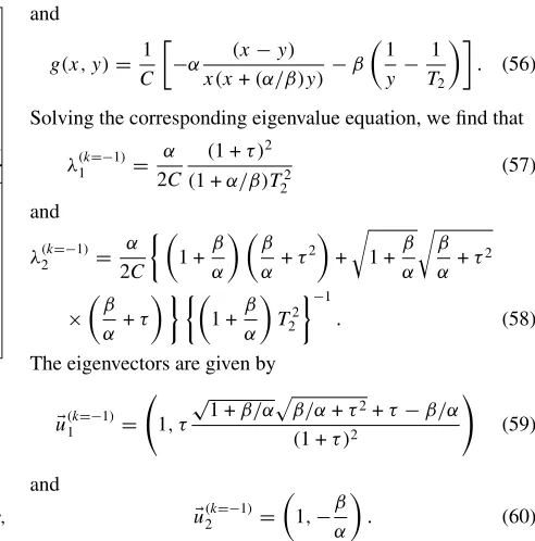
1 y − 1 T2 . (56) Solving the corresponding eigenvalue equation, we find that
λ(k1=−1)= α
2C
(1 +τ )2
(1 +α/β)T22 (57)
and
λ(k2=−1)= α
2C 1 +
β α β α+τ 2 +
1 +β
α β α +τ 2 × β α+τ
1 +β
α
T22
−1
. (58) The eigenvectors are given by
u(k1=−1)=
1, τ
√
1 +β/αβ/α+τ2+τ−β/α
(1 +τ )2
(59)
and
u(k2=−1)=
1,−β
α
. (60) By using the definition of characteristic time scale given by equations (9) and (10) one finds that
t1(k=−1)= 2C
|α|
(1 +α/β)T22
(1 +τ )2 (61) and
t2(k=−1)= 2C
|α| 1 +
β α
T22 1 +
β α β α +τ 2 +
1 + β
α β α +τ 2 β α +τ −1 . (62) In equations (57) and (58) one can observe that the eigenvalues
are negative becauseαandβ are negative; then, the system
is stable for every value of C and τ. That is, every small
perturbation around the steady-state values of temperaturex¯
andy¯decays exponentially with time. Eigenvectors given by
equations (59) and (60) represent the directions along which relaxation times can be defined by equations (61) and (62). In
figures 7(a) and 7(b) we plot the relaxation times againstτfor
several values of the ratioβ/α, for a fixed value ofα. For a
given value of the ratioβ/α, we observe that both relaxation
times decrease asτincreases; that is, the stability improves as
τ → 1. In the regionβ/α 1, as the ratioβ/α decreases
(figure 7(a)), the relaxation timet1(k=−1)increases. In the limit
β/α→0,t1(k=−1)→ ∞and the stability is lost. Ifβ/α >1,
both relaxation times decrease (see figure 7(b)).
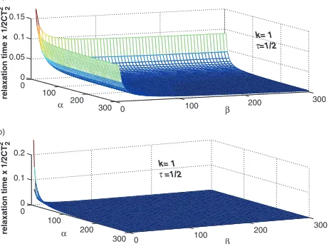
In figures 8(a) and (b) we present the plot of relaxation
times againstαandβ, with a fixed value ofτ = 12. In this
case,t1(k=−1)diverges whenα→0 orβ→0. In the region of
large values ofαandβ,t1(k=−1)is zero (see figure 8(a)). On
the other hand,t2(k=−1)is a decreasing function ofαandβ. In
particular,t2(k=−1)diverges asα→0 andβ→0. In the limit
β → ∞andα → ∞,t2(k=−1)tends to zero. It follows that
the stability of the system declines in the limitsβ/α→0 and
α/β→0.
In the present case, 0 < t2(k=−1) < t1(k=−1), this means
t2 t1
t2 t1
0 0.2 0.4 0.6 0.8 1
τ 0 0.2 0.4 τ0.6 0.8 1
0 5 10
relaxation times (x
α/
CT
2
)
}
k =–1 k =–1
0 0.5 1 1.5 2 2.5 3 (b) (a)
}
}
β/α= 1
β/α= 0.5
β/α= 0.3
β/α= 0.1
β/α= 3
β/α= 5
β/α= 8
β/α= 10
2
relaxation times (x
α/
CT
2
)
[image:7.595.65.538.75.252.2]2
Figure 7.Plot of relaxation times versusτfor some values of the ratioβ/α, with a fixed value ofα. The relaxation timest1(k=−1)andt2(k=−1)
are decreasing functions ofτ. (a) As the the ratioβ/α1 decreases both relaxation times increase. (b) Ifβ/α >1, both relaxation times decrease. Similar plots can be obtained if one assumes a fixed value ofβ >0 and variesα.
100 200
300 0 100 200
300 β
α
β α
100 200
300 0 100
200 300
0 0 0.05 0.1 0.15
0 0 0.1 0.2
relaxation time x 1/2CT
2 2
relaxation time x 1/2CT
2 2
k= 1 τ=1/2
k= 1 τ =1/2 (a)
(b)
Figure 8.Plots of relaxation times againstαandβforτ=1 2. (a) The relaxation time (t1(k=−1)) diverges asα→0 for every value ofβand vice versa. (b) The relaxation time (t2(k=−1)) diverges asα
andβapproach the origin and decreases asαandβincrease.
slow eigendirection (equation (61)) and a fast eigendirection (equation (62)). In figure 9 we present a qualitative phase
portrait of the caseβ = α withτ = 0.5. The trajectories
approach the origin tangent to the slow eigendirection and in backwards time the trajectories are parallel to the fast
eigendirection. A different situation arises whenβ/α =0.1,
that is,β < α. In this case (figure 10), the fast eigendirection is
close to the horizontal axis whereas the slow eigendirection is
close to the vertical axis. Thus, any perturbation in thexandy
values tends to come back to the steady state, decreasing very
quickly the temperaturexin comparison to the temperaturey.
The opposite situation occurs whenβ/α =10, that is, when
βis larger thanα. In this case (figure 11), the temperaturey
decays almost instantaneously whereasxdecays slowly.
4.3. Case k=4
In this case, equations (13) and (14) are in the form of the Stefan–Boltzmann law. Now, the efficiency that maximizes
x y
fast eigendirection
slow eigendirecti on
β/α = 1 τ = 1/2
[image:7.595.305.536.307.474.2]k =–1
Figure 9.Qualitative phase portrait ofx(t )versusy(t )forβ=α
andτ= 1
2. In this case, 0< t (k=−1) 2 < t
(k=−1)
1 and the ratio
t1(k=−1)/t2(k=−1)≈2.1. The corresponding eigenvectors can be described as the fast eigendirection (equation (60)) and the slow eigendirection (equation (59)). The eigendirections are
u(k1=−1)=(1,0.25)andu(k2=−1)=(1,−1). This is an interesting case, the fast eigendirection has slope equal to−1. For this reason, the decaying rates are almost equal, and, near the origin, the trajectories approach tangent to the slow eigendirection.
the power output cannot be written in closed form because the
solutionηcorresponds to an eighth-degree equation [1]. Let
us consider the significant case whenβ→ ∞, that is, the ratio
α/β→0. In this limit, the internal temperaturex¯is involved
in the well-known formula in solar energy conversion [6, 7]:
4x¯5−3T2x¯4−T14T2=0. (63)
Moreover, it has been reported that numerical calculations lead to the description of the behaviour of the
maximum-power efficiencyηas a decreasing function ofτ [1, 6]. An
approximate expression could be stated, in principle, for the
efficiency withτ. In this sense, some expressions have been
proposed for the maximum efficiency [13]. Here, we will use the efficiency proposed by Landsberg–Petala–Press [13]
¯
[image:7.595.64.295.315.486.2]β/α = 0.1 τ = 1/2
fast eigendirection
slow eigendirection
k= –1
[image:8.595.64.295.82.242.2]x y
Figure 10.Qualitative phase portrait ofx(t )versusy(t )for
β/α=0.1 andτ= 1
2. In this case, the ratiot (k=−1)
1 /t
(k=−1) 2 ≈3.3. The slow eigendirection (equation (59)) and the fast eigendirection (equation (60)) areu(k1=−1)=(1,2.3)andu(k2=−1)=(1,−0.1), respectively. The fast eigendirection is almost parallel to the horizontal axis and the slow eigendirection has a positive slope (≈2.3). For this reason,x(t )decays quickly whereasy(t )decays slowly.
fast eigendirection
slow eigendirection τ =1/2
β/α =10
x y
k =–1
Figure 11.Qualitative phase portrait ofx(t )versusy(t )for
β/α=10 andτ=1
2. In this case, the ratiot (k=−1)
1 /t
(k=−1) 2 ≈9.9. The slow eigendirection (equation (59)) and the fast eigendirection (equation (60)) areu(k1=−1)=(1,0.02)andu(k2=−1)=(1,−10), respectively. As we can see, the fast eigendirection is almost parallel to the vertical axis (y) and the slow eigendirection is parallel to the horizontal axis (x). It follows that,y(t )decays almost
instantaneously whereasx(t )decays slowly.
Equating equations (20) and (equation (64)), and solving for a
real value ofτ, we obtain
τ= H (√x,¯ y)¯
2 −
1 2
4√2
H (x,¯ y)¯ −2H
2(x,¯ y),¯ (65) with
H (x,¯ y)¯ =
y¯+(x¯3/2+x¯3− ¯y3)2/3
√ ¯
x(x¯3/2+x¯3− ¯y3)1/3. (66)
In the limitα/β → 0, equations (16) and (17), that is, the
steady-state valuesx¯andy¯take the form
¯
x= T2
(4/3)τ−(1/3)τ4, (67) ¯
y=T2. (68)
0 0.2 0.4 0.6 0.8 1
τ 0
0.05 0.1 0.15 0.2 0.25 0.3 0.35 0.4
relaxation time x (4
α
/C)T
2 α/β→0
k =4
[image:8.595.302.536.82.247.2]3
Figure 12.Plot of relaxation time versusτfor the caseα/β→0 andk=4. The relaxation time is a convex curve as a function ofτ.
In the limitα/β →0 andk=4, equation (24) permits us to
express the steady-state power output as
¯
P (x,¯ y)¯ =α(x¯− ¯y)(y¯
4− ¯x4τ4) ¯
xτ4 , (69)
whereτis given by equation (65). It is clear from equation (68)
that the steady-state temperaturey¯equals the temperature of
the cold reservoir. For this reason, the two-dimensional system given by equations (29) and (30) becomes a one-dimensional
system given only by the change in time of the temperaturex,
that is,
dx
dt =
1
C α(T
4 1 −x
4)−αy4−x4τ4
τ4
, (70) where we have used equation (69) and the assumption that
the power output has anx dependence similar in form to the
power in the steady-state conditions. To analyse the local
stability we takef (x)as the right-hand side of equation (70).
We proceed following typical procedures for the local stability analysis of a one-dimensional system. It is easy to show that, after assuming a small perturbation around the steady-state value, a linear relationship can be stated for the perturbation. To see whether the perturbation grows or decays, we must
calculatef(x)¯ , wherex¯is given by equation (67). Moreover,
the relaxation time is given by the reciprocal 1/|f(x)¯ |. After
the calculations described above, we found that f(x)¯ is
negative for 0 < τ < 1, that is, the system is stable. In
figure 12 we plot the relaxation time againstτ. We observe
that the relaxation time is a convex curve ofτ. It follows that
the stability improves whenτapproaches the origin or one.
5. Concluding remarks
We have presented a local stability analysis of an endoreversible CAN engine. It is important to discuss the stability characteristics of the endoreversible engine from the energy perspective.
The steady-state efficiency is a function ofτand the ratio
β/α. In figure 13 we plot the efficiency against the ratioβ/αfor
both casesk=1 (equation (31)) andk= −1 (equation (47))
[image:8.595.68.286.338.490.2]0
0 2 4 6 8 10
0.2 0.4 0.6 0.8 1
β/α
Efficiency
k =–1
[image:9.595.65.293.72.250.2]k =1
Figure 13.Plots of the steady-state efficiency against the ratioβ/α. In the casek=1 the efficiency is constant whereas ink= −1, the efficiency is a decreasing function of the ratioβ/α.
0 (b)
0.2 0.4 0.6 0.8 1 (a)
power output x 2/
α
T1
power output x 2/
α
T2
0 0.2 0.4 0.6 0.8 1
τ 0
0.2 0.4 0.6 0.8
k =1
[image:9.595.301.537.81.253.2]k =−1
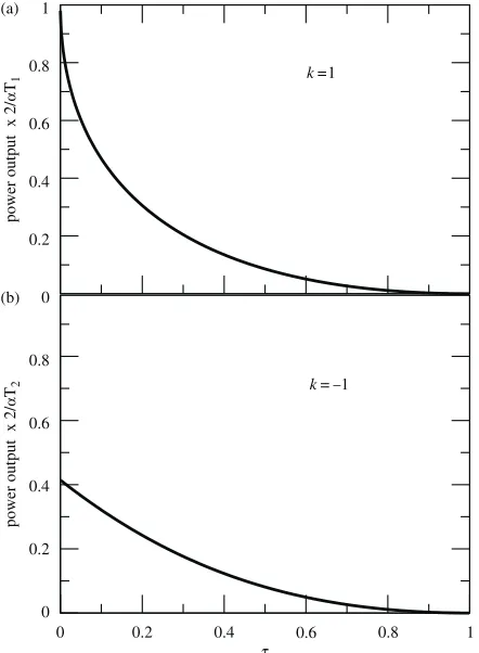
Figure 14.Plots of power output againstτ. In both cases ((a) and (b)), the power outputs are decreasing functions. In the limitτ→1, the power output is zero in both cases.
the case of Newton’s law (k=1) does not depend on the ratio
β/α. Whenk= −1, the efficiency is a decreasing function of
β/α. The steady-state power output and the efficiency are also
functions ofτ. In figures 14(a), 14(b) and 15 we plot these
energy functions versusτfor both casesk=1 (equations (32)
and (31)) andk= −1 (equations (48) and (47)) withα =β.
The power and the efficiency are decreasing functions ofτ.
From these considerations, one can conclude that the stability
of an endoreversible engine improves asτincreases, whereas
0 0.2 0.4 0.6 0.8 1
τ 0
0.2 0.4 0.6 0.8 1
Efficiency
k =1
k =–1
Carnot
[image:9.595.67.288.307.608.2]k =4
Figure 15.Plot of steady-state efficiency againstτ. For the cases
k=1 andk= −1, we considerα=β. For the casek=4, the approximate steady-state efficiency depends neither onαnor onβ. In all the cases, efficiencies decrease asτincreases. In the limit
τ→1, the efficiencies are zero.
the power and efficiency decrease in both cases (k = 1 and
k = −1). It is interesting that the minimum value for the
relaxation time at√τ =α/βis observed for the casek=1.
On the other hand, the efficiency is constant (casek=1), and is
a decreasing function (casek= −1) of the ratioβ/α, whereas
the stability, in both cases, declines asα/β→0 orβ/α→0.
Physically, the limitsβ/α → 0 andα/β → 0 correspond
to reversible absorption of heat and reversible release of heat, respectively. Our local analysis reveals that in these limits, for
the casesk = 1 andk = −1, any small perturbation in the
internal temperature (yin the case of absorption andxin the
case of release) decays very slowly—in fact, the time to return to the steady-state temperature is infinity. For this reason the system loses its stability. At the same time, the temperature
(xin the case of absorption andyin the case of release) decays
almost instantaneously.
Finally, we have analysed the casek = 4 in the limit
β → ∞. In this case, we observe that the relaxation time
is a convex curve when plotted as a function of τ and the
efficiency is a decreasing function of τ (see figure 12). It
is remarkable that typical devices powered by solar radiation
operate between temperaturesT1 =5762 K andT2=288 K,
that is, τ = 0.049 98 [1, 13]. At this value, according to
figure 12, the relaxation time is very small and the stability is high.
Acknowledgments
We thank M Santill´an and F Angulo for stimulating discussions, suggestions and invaluable help in the preparation of the manuscript. We also thank L Arias, J Edge, R Mota and D Stouffer. This work was supported in part by COFAA-IPN, EDI-IPN, M´exico.
References
[2] Sieniutycs S and Salamon P (ed) 1990Finite Time Thermodyn-amics and Thermoeconomics(London: Taylor and Francis) [3] Bejan A 1996Entropy Generation Minimization(Boca Raton,
FL: CRC press)
[4] Curzon F L and Ahlborn B 1975Am. J. Phys.4322 [5] Rubin M H 1979Phys. Rev.A191277
[6] De Vos A 1985Am. J. Phys.53570–3
[7] Chen L and Yan Z 1989J. Chem. Phys.903740–3 [8] Arias-Hern´andez L A and Angulo-Brown F 1997J. Appl.
Phys.812973
[9] Daw C Set al1998Phys. Rev.E572811–19
[10] Santill´an M, Maya-Aranda G and Angulo-Brown F 2001
J. Phys. D: Appl. Phys.342068–72
[11] Strogatz H S 1994Non Linear Dynamics and Chaos: With Applications to Physics, Chemistry and Engineering
(Cambridge, MA: Perseus)
[12] Arias-Hern´andez L A 1995MSc ThesisESFM, Instituto Polit´ecnico Nacional, M´exico