Essays on marital sorting and fertility

Texto completo

(1)Essays on Marital Sorting and Fertility. Marc Goñi i Tràfach TESI DOCTORAL UPF / ANY 2014. DIRECTOR DE LA TESI. Hans-Joachim Voth, Departament d’Economia i Empresa.

(2)

(3) To Josep Tràfach i Carreras. iii.

(4)

(5) Acknowledgements My first thanks goes to my advisor Hans-Joachim Voth for his continuous encouragement over the last six years. His guidance through all the stages of this work was invaluable. I owe much gratitude to Joel Mokyr for hosting me at Northwestern University. I am grateful to Albrecht Glitz and Giacomo Ponzetto, whose support and helpful comments I highly appreciate. Additional thanks go to Ran Abramitzky, Sasha Becker, Dan Bogart, Davide Cantoni, Deborah Cohen, Mauricio Drelichman, Jan Eeckhout, Nancy Ellenberger, Gabrielle Fack, Ray Fisman, Gino Gancia, Albrecht Glitz, Regina Grafe, Boyan Jovanovic, Peter Koudijs, Lee Lockwood, David Mitch, Thomas Piketty, Gilles Postel-Vinay, Giacomo Ponzetto, and John Wallis. I am indebted to the participants of the international lunch at CREI, the LPD seminar at UPF, the applied lunch and the economic history lunch at NWU. In addition, I want to thank the seminar participants at PSE, Belgrade (National Bank of Serbia Conference), Rome (MOOD workshop), Galway (Applied micro conference), Malaga (EEA meetings), York (EHS meetings), Orange (All-UC economic history conference) Honolulu (World Congress of Cliometrics), and Washington (EHA meetings). I would like to express my gratitude to the Department of Economics, Universitat Pompeu Fabra and to the Agència de Gestió d’Ajuts Universitaris i de Recerca (FI grant 2012 00796) for their financial support. I acknowledge the Cambridge Group for the History of Population and Social Structure for kindly allowing me to use the Hollingsworth dataset. In addition, I would like to thank Marta Araque and Laura Agustı́ at GPEFM, and Mariona Novoa at CREI for their superb administrative support. Many thanks to my PhD colleagues and friends Alain, Paul, Pietro, Gene, Mapis, Lorenzo, Anna, Patty, Alberto, Pau, José-Antonio, Narly, Stefan, and Matranga. A special mention goes to Fernando, Jörg, Miguel, and Priscilla. My regards to the family and friends of Cédric and Michael. Finally, let me express my warm thanks to Héctor, Carlos, Maria, my parents, my sister, and Emma. Això és vostre també!. v.

(6)

(7) Abstract This thesis examines the interactions between marital patterns, inequality, and fertility. In the first chapter I analyze the impact of search frictions on marital assortative matching. I exploit a temporary interruption of the “London Season” — a central marriage market where the nineteenthcentury British aristocracy courted. I find that the reduction of search frictions associated with this institution explains between 70 and 80 percent of sorting in social status and land-holdings, generating a huge concentration of landed wealth. In the second chapter I examine the relationship between land inequality and the introduction of public education in lateVictorian England and Wales. I show that counties where landownership was more concentrated systematically under-invested in public schooling. In the final chapter I estimate the effects of cousin marriage on fertility in the British peerage. I find that consanguinity initially increases the number of births, but constraints reproductive success in the long-run.. Resum En aquesta tesis s’examina la interacció entre els patrons matrimonials, la desigualtat i la fertilitat. En el primer capı́tol s’analitza l’impacte de les friccions en el procés de cerca sobre l’emparellament selectiu. L’anàlisi es centra en una interrupció de la “London Season” — un mercat de matrimonis centralitzat on els nobles Britànics buscaven esposa. S’estableix que la reducció en les friccions de cerca associades a aquesta institució explica entre un 70 i un 80 per cent de l’emparellament selectiu en termes d’estatus social i de terratinença, afavorint la concentració de terres en poques mans. Al segon capı́tol s’examina la relació entre la desigualtat en la distribució de la terra i la introducció de l’educació pública a l’Anglaterra victoriana. Els resultats indiquen que els comptats més desiguals varen patir un dèficit sistemàtic en educació pública. Al capı́tol final s’estimen els efectes de l’endogàmia sobre la fertilitat a la noblesa Britànica. L’endogàmia sembla augmentar el nombre de naixements, però alhora limita l’èxit reproductiu en el llarg termini. vii.

(8)

(9) Preface On 29 April 2011, the daughter of a former flight attendant married the future king of England. The wedding of Kate Middleton to Prince William, however, was rather an exception. One of the hallmarks of modern marriage in OECD countries is that people tend to marry other people who have similar education, income, or social status (Chen et al. 2013). From an economic perspective, who marries who has important implications for fertility and education, and ultimately affects the distribution of wealth within a society. In recent years a flourishing literature has arisen on both the causes and the effects of marital sorting (see Fernandez and Rogerson 2001, Fernandez et al. 2005, Fisman et al. 2008, Hitsch et al. 2010, Greenwood et al. 2014 and references therein). One of the most important questions in this literature is where sorting comes from. Homophily — a preference for others who are like us — is only one reason for assortative matching. Every relationship not only reflects who we chose but also depends on who we meet. Do the “rich” marry each other because they have a taste for money, or just because they go to the same bars, attend the same schools, or live in the same neighborhoods? Assignment theory suggests a strong link between these search frictions and marital sorting (Collin and McNamara 1990, Burdett and Coles 1997, Eeckhout 1999, Shimer and Smith 2000, Bloch and Ryder 2000, Adachi 2003, Atakan 2006, Jacquet and Tan 2007). Notable papers have tested this relation using speed dating (Fisman et al. 2008) or dating websites (Hitsch et al. 2010). Although such modern-day datasets contain a lot of information, they present several shortcomings. Dating is not marriage; in most cases, it does not lead to long-term partnerships. Also, nowadays we continuously interact with people from the opposite sex, in a multitude of settings. As a consequence, we can only observe imperfectly who is actually on the marriage market and who meets whom. Going back to history can be most helpful in solving these issues. I turn to a unique historical setting to study marital sorting. In the nineteenth century, for seven months each year, Parliament was in session and ix.

(10) the British elite converged on London. Their offspring participated in a string of social events designed to introduce rich and influential bachelors to eligible debutantes. This “matching technology,” known as the London Season, reduced search costs for partners. After the death of Prince Albert, however, the Season was interrupted for three consecutive years (1861–63). The first chapter of my thesis exploits this exogenous shock to identify the effect of search frictions on marital sorting. My results suggest that the link is strong: between 70 and 80 percent of sorting in social status and land-holdings in the nobility was explained by the reduction in search frictions associated with the London Season. Apart from its causes, the literature on marital sorting is also concerned with its economic consequences. There is a large body of work using modern-day data to evaluate the impact of marital sorting on inequality (see Kremer 1997, Fernandez and Rogerson 2001, Fernandez et al. 2005, Greenwood et al. 2014). The advantage of using historical data is that it sheds light on the nature of this interaction in the long-run. My results suggest that marital sorting was important in perpetuating the English nobility’s role as an unusually small, exclusive, and rich elite. In detail, marital sorting and inequality of landownership reinforced each other over centuries. This allowed the British peerage to accumulate the lion’s share of land.1 In the second chapter of my thesis I evaluate whether this huge concentration in landownership was harmful for Britain’s performance. By 1860, it did not seem so: Britain was the first industrial country and the world’s workshop. However, the provision of public education lagged behind Prussia and the United States, nations that eventually overtook the world’s industrial leadership (McCloskey and Sandberg 1971). Why was public education not established earlier on? Sokoloff and Engerman (2000) famously suggested that where land is unequally distributed, institutions may end up in the back pockets of landowners. This may slow down the provision of public schooling, since landowners do not need their farmers to be educated and want to reduce labor mobility. This ex1. Around 1880, fewer than 5,000 landowners still owned more than 50 percent of all land (Cannadine 1990).. x.

(11) planation seems particularly suited for England given the way in which public education was introduced for the first time: it was to be funded through local property taxes (rates). In theory, where landowners held most of the land, they had to effectively pay for all of the education. In practice, they took over School Boards — the public bodies in charge of raising funds for education locally — and undermined the provision of public schooling. Exploiting the rich reports of the Committee of Council on Education, I find that School Boards located in counties where landownership was more concentrated systematically under-invested in public schooling and present worse educational outcomes. In contrast, counties with a large share of manufacturing employment were more eager to subsidize public education, reflecting a clash between peer landowners and emerging industrialists. Hence, the concentration of landed wealth associated with marital sorting crucially contributed to undermine the introduction of effective public schooling in England and Wales. Besides inequality and education provision, marriage patterns may also have important effects on fertility (Fernandez and Rogerson 2001). In the third chapter of my thesis I exploit the vast genealogical material on the British Peerage to shed light on the consequences of cousin marriage. Despite being widespread in developing societies2 cousin marriage has seldom been considered in the economic literature. Existing empirical evidence on the effect of consanguinity on fertility is contradictory and does not always confirm the stigma that the Western world has attached to cousin marriage. When estimating this relation, one should not ignore that consanguineous unions may confer greater reproductive success through earlier age at marriage or by preserving landholdings and wealth within the family. This is particularly important in communities with large socio-economic disparities, which also happen to be those with higher rates of consanguinity. A second key challenge is unobserved heterogeneity. Unobserved characteristics affecting the decision to marry a cousin may be correlated with unobservable factors influencing 2. Estimates suggest that more than 10 percent of people worldwide are either married to a close relative or are the offspring of such a marriage (Bittles 2012).. xi.

(12) fertility, such as personality, intelligence, or beauty (Kim 2013). I address these empirical challenges by exploiting the interruption of the London Season (1861–63) and the shift in marriage decisions to local markets populated by blood-related noblemen. Cousin marriage blossomed, and these unions gave birth to more offspring. However, the time elapsed from marriage to the first birth increased, indicating a larger probability of miscarriage. The children of consanguineous unions were less likely to reach the typical age at which noblemen married, had fewer children, and were 50 percent more likely to be childless. Thus, although consanguinity may have an initial positive effect on fertility, it is offset in the next generation, severely constraining reproductive success in the long-run. Throughout these three chapters, my thesis pins down the determinants as well as the effects of marital sorting in nineteenth-century Britain. Admittedly, this thesis looks at a very specific historical setting. Nonetheless, today’s marriage markets are not free of segregation. Sixty percent of Americans met their future partners at school, at work, at a private party, at church, or at a social club (Laumann et al. 1994, Table 6.1). In these marriage markets, entry is somehow restricted to similar others. Dating agencies that cater to rich clients are also spreading across the world. Seventy Thirty, for example, requires that both male and female members have assets worth £1m. In a world were the top 1 percent income share has already more than doubled over the last decades (Piketty and Saez 2006), evaluating the interaction between such segregative marriage practices, inequality, and fertility is crucial. My thesis shows that historical idiosyncrasies, such as the unique way in which the British aristocracy courted, can be used to shed light on these important questions.. xii.

(13) Contents. List of figures. xviii. List of tables 1. xx. Assortative Matching and Persistent Inequality: Evidence from the World’s Most Exclusive Marriage Market 1.1 Introduction . . . . . . . . . . . . . . . . . . . . . . . . 1.2 Historical background: the London Season . . . . . . . . 1.3 Data sources . . . . . . . . . . . . . . . . . . . . . . . . 1.3.1 Peerage records . . . . . . . . . . . . . . . . . . 1.3.2 Family seats . . . . . . . . . . . . . . . . . . . 1.3.3 Bateman’s Great Landowners . . . . . . . . . . 1.3.4 Lord Chamberlain’s records . . . . . . . . . . . 1.4 Empirical analysis . . . . . . . . . . . . . . . . . . . . . 1.4.1 Data descriptives . . . . . . . . . . . . . . . . . 1.4.2 Variation in the size of the cohort . . . . . . . . 1.4.3 The interruption of the Season, 1861–63 . . . . . 1.5 Robustness . . . . . . . . . . . . . . . . . . . . . . . . 1.5.1 Sample stratification . . . . . . . . . . . . . . . 1.5.2 Alternative measures of the Season . . . . . . . 1.5.3 The 22-year-old threshold . . . . . . . . . . . . 1.5.4 Assessing selection on unobservables . . . . . . 1.5.5 Plausibly exogenous instrument . . . . . . . . . 1.6 Discussion . . . . . . . . . . . . . . . . . . . . . . . . . 1.7 Economic implications in the long-run . . . . . . . . . . xiii. 1 1 10 15 15 17 18 19 19 20 24 31 36 37 38 38 39 41 42 44.

(14) 1.7.1 Sorting and inequality . . . . . . . . 1.7.2 Provision of public schooling . . . . 1.8 Model . . . . . . . . . . . . . . . . . . . . . 1.8.1 Standard two-sided search model . . 1.8.2 Matching technology . . . . . . . . . 1.8.3 Market segregation . . . . . . . . . . 1.9 Conclusion . . . . . . . . . . . . . . . . . . 1.10 Figures and tables . . . . . . . . . . . . . . . 1.11 Appendix A: Supplemental figures and tables 1.12 Appendix B: Proofs . . . . . . . . . . . . . .. . . . . . . . . . .. . . . . . . . . . .. . . . . . . . . . .. . . . . . . . . . .. . . . . . . . . . .. . 44 . 47 . 49 . 49 . 53 . 55 . 60 . 63 . 98 . 103. 2. Landed Elites and Public Education in England and Wales: Evidence from School Boards, 1870-99 109 2.1 Introduction . . . . . . . . . . . . . . . . . . . . . . . . 109 2.2 Literature review and contribution . . . . . . . . . . . . 113 2.3 Historical background . . . . . . . . . . . . . . . . . . . 117 2.4 Data . . . . . . . . . . . . . . . . . . . . . . . . . . . . 121 2.4.1 Reports of the Committee of Council on Education 121 2.4.2 Bateman’s Great Landowners . . . . . . . . . . 124 2.5 Empirical analysis . . . . . . . . . . . . . . . . . . . . . 126 2.5.1 The relationship between land inequality and education . . . . . . . . . . . . . . . . . . . . . . 126 2.5.2 Political channel? Peer vs. commoner landowners 130 2.6 Robustness . . . . . . . . . . . . . . . . . . . . . . . . 132 2.6.1 Sample stratification . . . . . . . . . . . . . . . 132 2.6.2 Assessing selection on unobservables . . . . . . 133 2.7 Conclusion . . . . . . . . . . . . . . . . . . . . . . . . 134 2.8 Figures and tables . . . . . . . . . . . . . . . . . . . . . 137 2.9 Appendix A: Examination standards . . . . . . . . . . . 157. 3. Kissing Cousins: Estimating the Causal Effect of Consanguinity on Fertility Using Evidence from the London Season 159 3.1 Introduction . . . . . . . . . . . . . . . . . . . . . . . . 159 3.2 Historical background . . . . . . . . . . . . . . . . . . . 166 xiv.

(15) 3.3 3.4 3.5. 3.6 3.7 3.8. 3.2.1 Cousin marriage in Britain . . . . . . . . . . . . 3.2.2 The London Season . . . . . . . . . . . . . . . . Identification strategy . . . . . . . . . . . . . . . . . . . Data . . . . . . . . . . . . . . . . . . . . . . . . . . . . Results . . . . . . . . . . . . . . . . . . . . . . . . . . . 3.5.1 The interruption of the Season and cousin marriage, 1861–63 . . . . . . . . . . . . . . . . . . 3.5.2 The effect of consanguinity on fertility . . . . . Conclusion . . . . . . . . . . . . . . . . . . . . . . . . Figures and tables . . . . . . . . . . . . . . . . . . . . . Appendix A: Supplemental figures and tables . . . . . .. xv. 166 167 168 171 172 172 175 180 182 194.

(16)

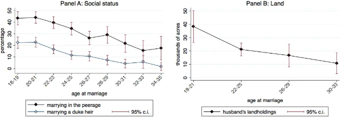
(17) List of Figures 1.1 1.2 1.3 1.4 1.5 1.6 1.7 1.8 1.9 1.10 1.11 1.12 1.13 1.14 1.15 1.16 1.17 1.18 1.19. The effects of the interruption of the Season on the relative probability of marrying outside the peerage . . . . . 63 Seasonable Migrations of the “Fashionable World”, 1841 64 Country seats . . . . . . . . . . . . . . . . . . . . . . . 65 Number of attendees at royal parties, by type of event . . 66 Network of peer landowners and their spouses, 1868. . . 67 Implied market value of women by age group, 1801–75. 68 Increasing returns to scale in the London Season. . . . . 69 The effects of the interruption of the Season on peer-commoner intermarriage . . . . . . . . . . . . . . . . . . . . . . . 70 Deferred marriage decision of ladies aged below 22 in 1861 71 The effects of the interruption of the Season on husbands’ landholdings . . . . . . . . . . . . . . . . . . . . . . . . 72 The effects of the interruption of the Season on sorting in acreage . . . . . . . . . . . . . . . . . . . . . . . . . . 73 The effects of the interruption of the Season on the distance between spouses’ seats . . . . . . . . . . . . . . . 74 Relaxing the 22-year threshold . . . . . . . . . . . . . . 75 Political endogamy and the London Season . . . . . . . 76 Marrying outside the peerage without the Season . . . . 77 Sorting and inequality . . . . . . . . . . . . . . . . . . . 78 Kernel density for investments in education, 1873-94 . . 79 Increasing efficiency of the matching technology . . . . 80 Segregation in the marriage market . . . . . . . . . . . . 81 xvii.

(18) 1.A1 Charles, 5th Baron Lyttelton, Cockayne’s Complete Peerage 98 1.A2 Charles, 5th Baron Lyttelton, Bateman’s Great Landowners 98 1.A3 Kernel-weighted local polynomial smoothing: Husband’s landholdings on wife’s landholdings, 1851–75 . . . . . . 99 1.A4 Hazard rates for the cohort marrying in 1850–59 . . . . . 99 1.A5 Relation between cohort size and royal parties . . . . . . 100 2.1. Relationship between land concentration and funds raised from rates . . . . . . . . . . . . . . . . . . . . . . . . . 137 2.2 School Board funding: Berkshire, 1883–84 . . . . . . . 138 2.3 School Board expenditures: Berkshire, 1883–84 . . . . . 138 2.4 Schooling outcomes: England, 1883–84 . . . . . . . . . 139 2.5 Funds from rates over time: top decile vs. bottom decile counties . . . . . . . . . . . . . . . . . . . . . . . . . . 140 2.6 Kernel density of the percentage of scholars passing the arithmetics, reading, and writing exams . . . . . . . . . 141 2.7 Lorenz curve for the land distribution in the average county 141 2.8 Share of land owned by peers across counties . . . . . . 142 2.9 Kernel density for funds from rates: counties with land concentration above vs. below the median . . . . . . . . 143 2.10 Funds raised from rates over time: counties with large vs. small land concentration, by status of the landowner . . . 144 3.1 3.2 3.3 3.4. Global prevalence of consanguineous marriages, 2001 . . 182 Seasonable migrations of the “Fashionable World”, 1841 183 Number of attendees at royal parties, by type of event . . 184 The effects of the interruption of the Season on the distance between spouses’ seats . . . . . . . . . . . . . . . 185 3.5 The effects of the interruption of the Season on cousin marriage . . . . . . . . . . . . . . . . . . . . . . . . . . 185 3.6 The effects of the interruption of the Season on consanguinity . . . . . . . . . . . . . . . . . . . . . . . . . . . 186 3.7 Relationship between consanguinity and number of children186 3.A1 Knot system for relative consanguinity . . . . . . . . . . 194. xviii.

(19) List of Tables 1.1 1.2 1.3 1.4 1.5 1.6 1.7 1.8 1.9 1.10 1.11. 1.15 1.16 1.A1 1.A2. Marriage outcomes for peers and peers’ sons, 1801–1875 82 Marriage outcomes for peers’ daughters, 1801–1875 . . 83 Marriage outcomes by family pedigree, 1814–75† . . . . . 84 Sorting by acreage for great landowners, 1838–75† . . . 85 Sorting by land rents for great landowners, 1838–75† . . 86 Geographic endogamy by social group, 1801–75 . . . . 87 The Season and sorting by social position . . . . . . . . 88 The Season and sorting by landholdings . . . . . . . . . 89 The Season and socio-economic homogamy . . . . . . . 90 The Season and geographic endogamy . . . . . . . . . . 91 Balanced cohorts: Interruption of the Season vs. normal years . . . . . . . . . . . . . . . . . . . . . . . . . . . . 92 Sample stratification . . . . . . . . . . . . . . . . . . . 93 Alternative measures of attendance to the Season . . . . 94 Using selection from observables to assess the selection on unobservables . . . . . . . . . . . . . . . . . . . . . 95 IV estimates for plausibly exogenous cohort size instrument 96 Marriage and political preferences, 1817–1875† . . . . . 97 Relation to landowner of matched wives . . . . . . . . . 101 Marital network connections, 1862 . . . . . . . . . . . . 102. 2.1 2.2 2.3 2.4. Elementary Education Acts, 1870–1902 . . Descriptive statistics . . . . . . . . . . . . Land distribution in the average county . . . Land concentration and funds for education. 1.12 1.13 1.14. xix. . . . .. . . . .. . . . .. . . . .. . . . .. . . . .. . . . .. 145 146 147 148.

(20) 2.5 2.6 2.7. Land concentration and education expenditures . . . . . Land concentration and education outcomes . . . . . . . Land concentration and funds for education, by status of the landowner (peer vs. commoner) . . . . . . . . . . . 2.8 Land concentration and education expenditures, by status of the landowner (peer vs. commoner) . . . . . . . . . . 2.9 Land concentration and education outcomes, by status of the landowner (peer vs. commoner) . . . . . . . . . . . 2.10 Sample stratification . . . . . . . . . . . . . . . . . . . 2.11 Using selection from observables to assess the selection on unobservables . . . . . . . . . . . . . . . . . . . . . 2.A1 Examination standards . . . . . . . . . . . . . . . . . . 3.1. 149 150 151 152 153 154 156 157. The relationship between disruptions to the matching technology and consanguinity, 1859–67 . . . . . . . . . . . 187 3.2 Balanced cohorts: Interruption of the Season vs. normal years . . . . . . . . . . . . . . . . . . . . . . . . . . . . 188 3.3 The effect of consanguinity on the number of births, first generation . . . . . . . . . . . . . . . . . . . . . . . . . 189 3.4 The effect of consanguinity on other fertility outcomes, first generation . . . . . . . . . . . . . . . . . . . . . . 190 3.5 The effect of consanguinity on the number of births, second generation . . . . . . . . . . . . . . . . . . . . . . 191 3.6 The effect of consanguinity on the number of births by gender, second generation . . . . . . . . . . . . . . . . . 192 3.7 The effect of consanguinity on infertility, second generation193 3.A1 Summary statistics, first generation . . . . . . . . . . . . 195 3.A2 Summary statistics, second generation . . . . . . . . . . 196. xx.

(21) Chapter 1. Assortative Matching and Persistent Inequality: Evidence from the World’s Most Exclusive Marriage Market 1.1. Introduction. Dentists marry dentists, Hollywood stars marry each other, and economists marry economists. Marital assortative matching — the tendency of people of similar social class, education, and income to marry each other — has important implications for education and inequality (Fernandez and Rogerson 2001, Fernandez et al. 2005). To investigate these implications further, it is crucial to first understand what drives marital sorting. Homophily — a preference for others who are like ourselves — is only one reason for assortative matching. In addition, the people we meet also circumscribes the set of mates we can chose from. In other words, every 1.

(22) relationship not only reflects who we chose but also depends on who we meet. A robust prediction of marriage models is that search frictions affect marriage outcomes (Collin and McNamara 1990, Burdett and Coles 1997, Eeckhout 1999, Shimer and Smith 2000, Bloch and Ryder 2000, Adachi 2003, Atakan 2006, Jacquet and Tan 2007). Confirming this prediction with data is not straightforward. Recent empirical work has used speed dating (Fisman et al. 2008), marriage ads in newspapers (Banerjee et al. 2009), or dating websites (Hitsch et al. 2010). Results are at odds with the theory — preferences appear to be an important determinant of sorting, but the matching technology does not seem to clearly affect the outcomes. Does this discrepancy reflect flaws in search theory or in modern-day data? Dating is very different from marriage. In most cases, it does not reflect the long-term partnership formation at the core of search and matching theory (Diamond 1981, Mortensen 1993, 1988, Pissarides 1984, Mortensen and Pissarides 1994). Relating marriage outcomes to the matching technology is also complicated by the fact that the latter is hard to measure. In modern marriage markets, members of the opposite sex continuously interact in a multitude of settings. As a consequence, it is virtually impossible to isolate a particular matching technology from other courtship processes. In this paper, I use a unique historical setting to investigate these issues further. I examine the marriage strategies of the British upper classes in a search and matching framework. In the nineteenth century, from Easter to August every year, a string of social events was held in London to “aid the introduction and courtship of marriageable age children of the nobility and gentry”1 — the London Season. It was at the heart of the British upper class social life, and almost all of the peerage and gentry was involved. Courtship in noble circles was largely restricted to London; in most cases, the only place where a young aristocrat could speak with a girl was at a ball during the Season. Crucially, the Season was interrupted by a major, unanticipated, exogenous shock: the death of Prince Albert. When Queen Victoria went into mourning, all royal dinners, balls, and luncheons were cancelled for three consecutive years (1861–63). I use this large shock — 1. Motto of the London Season at londonseason.net.. 2.

(23) unrelated to the Season’s main function — to identify the effects of the Season on marriage outcomes. In addition, I exploit changes in the size of the marriageable cohort as a source of identifying variation. This allows me to quantify the magnitude of the gains in matching efficiency created by the Season in the long-run (1851–75). I find a clear, strong link between search costs and marital sorting. Using a combination of hand-collected and published sources on peerage marriages,2 I find that in years when the Season effectively reduced search costs, the nobility’s daughters sorted more in the marriage market: they were less likely to marry a commoner and were increasingly likely to marry husbands from families with similar landholdings. When the Season was disrupted, spouses came instead from geographically adjacent places, indicating that local marriage markets became a more important source of partners. There, markets were more shallow, reducing the strength of marital sorting. Once the forces behind marital assortative matching are identified, I turn to examine the broader economic implications of sorting. I look at the effects of the Season — and its implied marriage patterns — on social mobility, inequality, and the provision of public education. A counterfactual analysis shows that if the Season had not existed, marriages between peers’ daughters and commoners’ sons would have been 30 percent higher in 1851–75. The institutional innovation of the Season, thus, helped the British elite erect an effective barrier that kept out newcomers (Stone and Stone 1984). Without the Season, England would have looked much more like continental countries, with large and not very rich aristocracies. Because marriage is important for the intergenerational transmission of inequality, the Season also contributed to the extreme concentration of wealth in the hands of the British aristocracy. Compared to the nobility of many other countries, the British aristocracy not only “held the 2. I use the Hollingsworth genealogical data on the peerage to describe the marriage behavior of the British elite. Hollingsworth (1957 and 1964) compiled evidence on marriage and social status for 26,000 peers and their offspring for the period 1566–1956. I complement this dataset with additional information from two published sources and from the archives (see data section).. 3.

(24) lion’s share of land, wealth, and political power in the world’s greatest empire” (Cannadine 1990),3 its members towered over their continental cousins in terms of exclusivity, riches, and political influence. My results strongly suggest that a high degree of assortative matching contributed to this outcome. In a cross-section of English and Welsh counties, I find that where noble dynasties intermarried less with commoners over centuries, land was more unequally distributed. Economic inequality, in turn, can actually inflict a lot of harm on a country’s long-term economic prospects (Persson and Tabellini 1994). In this paper, I discuss the effects of landownership concentration on public schooling (Sokoloff and Engerman 2000, Galor et al. 2009). Counties where land was more concentrated systematically under-invested in public education. With Forster’s Education Act (1870), England recognized it was the role of the state to provide public education, which was to be subsidized mainly through property taxes (rates). This suggests that England and Wales fell behind in terms of educating the workforce because its entrenched landed elite, especially the anointed peers, was powerful enough to undermine the introduction of effective public schooling. The Season provides a unique setting to study the determinants and the implications of marital sorting because it allows me to open the “black box” of the matching technology. Marriage markets today are typically informal. We can only guess who is on the market and who meets whom. In contrast, the matching process embedded in the London Season was explicit. Before the Season started, young ladies aged 18 were presented to the Queen at court. This formal act was a public announcement of who was on the marriage market. The debutante was then introduced into society at the balls and concerts organized during the Season. The purpose of these events was twofold: first, to allow for frequent encounters between suitors, and second to limit entry to “desirable” candidates. Guests were carefully selected by social status, and the high cost involved in participating even excluded aristocrats if they were pressed for money.4 Overall, 3. Around 1880, fewer than 5,000 landowners still owned more than 50 percent of all land (Cannadine 1990). 4 The cost was driven by the need to host large parties in a stately London home; only. 4.

(25) the matching process greatly reduced search frictions for the children of Britain’s elite. Several unique features of the historical setting allow me to identify the effects of the matching technology on marriage outcomes. The death of Prince Albert in 1861 was an exogenous disruption of the Season with strong effects on marriage outcomes. Figure 1.1 illustrates the consequences in one particular dimension: the rate of intermarriage between peers and commoners. The chart plots the number of people attending royal parties in the Seasons between 1859 and 1867 and the percentage of marriages outside the peerage. The latter is presented as a ratio of the rate for women older than 22 in 1861 relative to women below this cutoff age. I separate these two groups because one would not expect younger ladies to be severely affected by the interruption of the Season; they could simply delay their choice of husband until everything went back to normal. However, women aged 22 and over in 1861 could not wait long if they wanted to avoid being written off as a failure based on the social norms of the time.5 Thus, they were forced to marry one of the first suitable suitors. Before Albert’s death and after the Season resumed, women in both age groups were equally likely to marry a commoner. However, a great gap between the two opens after 1861. Those who had to marry when the Season was disrupted performed much worse in the marriage market. Their likelihood of marrying a commoner was 80 percent higher than that of the younger ladies who could wait for the Season to resume. This suggests that the Season was highly effective as a matching technology — by announcing who was on the market, creating multiple settings for the opposite sexes to meet, and segregating the rich and powerful from the poor and insignificant, it crucially determined who married whom. My results contribute to the rich literatures on assortative matching those who issued invitations to balls, dinners, and luncheons could expect to receive them. 5 According to these norms, if a lady was not engaged two or three Seasons after “coming out” into society, she was written off as a failure (Davidoff 1973: p. 52). Furthermore, in the early 1860s most ladies married when between the ages of 22 and 25. Since the older cohort would be 25 or more when the Season resumed in 1864, waiting was not an option for them.. 5.

(26) and the importance of search costs. The study of marriage from an economic perspective dates back to the seminal works of Gale and Shapley (1962) and Becker (1973). These authors characterized the set of stable marriage assignments and derived the conditions for positive assortative matching. A classic insight from the assignment literature, however, is that once a search friction is introduced into the matching process, sorting is weakened or might even be lost. In other words, as the speed of encounters between singles increases, spouses will sort more in the marriage market (Collin and McNamara 1990, Burdett and Coles 1997, Eeckhout 1999, Bloch and Ryder 2000, Shimer and Smith 2000, Adachi 2003, Atakan 2006). In addition, Bloch and Ryder (2000) and Jacquet and Tan (2007) analyze endogenous market segmentation. They conclude that limiting people’s choice set to those who are most similar reduces the congestion externality, which refers to the time an agent spends meeting people with whom she will never match. Since people then meet desirable partners at a higher speed, sorting increases. Surprisingly, this well-accepted theoretical insight lacks clear-cut empirical support. Hitsch et al. (2010) estimate mate preferences from a dating website and then use the Gale-Shapley algorithm6 to predict frictionless matches. Since the predicted matches are as selective as those achieved by the dating site, they conclude that “assortative mating [in dates] arises in the absence of search frictions” (p. 162). The simulated matches also broadly resemble actual marriage patterns, although sorting by education or ethnicity are somewhat underpredicted. This suggests that search frictions would, in fact, increase sorting. Hitsch et al.’s (2010) result, however, may be explained by the fact that the preferences of online 6. The Gale-Shapley algorithm (Gale and Shapley 1962) involves a number of stages. In the first stage, each boy proposes to his most preferred girl. Each girl then replies “maybe” to her favorite suitor and “no” to all others. In the second stage, boys who were rejected propose to their second choices. Each girl replies “maybe” to her favorite among the new proposers and the boy on her string, if any. She says “no” to all the others (again, perhaps including her provisional partner). The algorithm goes on until the last girl gets her proposal. Each girl is then required to accept the boy on her string. This algorithm guarantees that marriages are stable, that is, no pair of woman and man prefers each other over their current partners.. 6.

(27) dating users differ from the preferences of the population at large.7 Lee (2008) obtains similar results in the context of a Korean match-making agency. Banerjee et al. (2009) estimate preferences for caste from marital advertisements in Indian newspapers. Their results suggest that search frictions play little role in explaining caste-endogamy on the arranged marriage market. Fisman et al. (2008) design a speed-dating experiment such that people of different ethnic groups meet at a high speed. The observed matches still display ethnic sorting, especially for women. This indicates that the low degree of interracial marriage in the Unites States stems not from segregation in the marriage market but from same-race preferences. In addition to preferences and the matching technology, several studies analyze sex ratios as a potential determinant of sorting. Abramitzky et al. (2011) show that after World War I, French males married up8 to a greater extent in regions where more men had died in the trenches. Angrist (2002) examines the effect of male-biased migration flows in the United States between 1910 and 1940 on various marriage and labor outcomes. Another set of related papers uses implicit differences in marriage market depth between the city and the countryside as a source of identifying variation. Gautier et al. (2010) look at migration flows in and out the city and find that it is a more attractive place to live for singles because it offers more potential partners. Botticini and Siow (2011) compare the city and countryside marriage markets in the United States, China, and early renaissance Tuscany. They find no evidence of increasing returns to scale in the matching function. While these papers analyze whether an agglomeration makes matching more efficient, I consider a different 7. Alternatively, the discrepancy between estimated frictionless matches and actual marriages may stem from methodological issues. First, the Gale-Shaply algorithm used to predict frictionless matches assumes nontransferable utility. This assumption appears appropriate to describe dating but not marriage, where explicit transfers play a large role nowadays. Furthermore, when estimating mate preferences, the authors rule out the possibility that there is noise in users’ behavior. Once they take this into account, results suggest that preferences alone explain all marital sorting (Hitsch et al. 2010: pp. 160). 8 That is, they married spouses of higher socio-economic status.. 7.

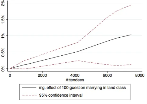
(28) matching technology. The Season not only pooled large numbers of eligible singles together, but it was also meant to facilitate their introduction and courtship. My findings suggest that this particular matching process displayed increasing returns to scale.9 This paper also sheds light on the relation between marital sorting, inequality, and economic growth. Although inequality is widely recognized as an important economic outcome, marital sorting has not received much attention as one of its potential determinants. Kremer (1997), Fernandez and Rogerson (2001), Fernandez et al. (2005), and Greenwood et al. (2014) establish a theoretical and empirical correlation between the degree to which spouses sort in the marriage market, economic inequality, and per capita incomes.10 Therefore, any process that increases inequality (e.g., skill-biased technological change) or reduces search costs for partners (e.g., Internet dating) could well lead to greater sorting and hence greater inequality. Because my paper considers a historical setting, I am able to analyze this relation in the very long-run. Understanding the longrun trend in inequality is important given the enormous concerns over this as a policy issue. Piketty and Saez (2006) use historical tax statistics to construct a long-run series for income and wealth concentration. For most Western democracies, they find a trend of increasing inequality over the last 25 years. High inequality, in turn, may have dramatic effects on important economic outcomes such as taxation (Persson and Tabellini 1994) or the provision of public education (Sokoloff and Engerman 2000), ultimately affecting the growth process. 9. In particular, when royal parties were attended by less than 2,000 guests, the probability of marrying a spouse with similar landholdings increased by 0.25 percent for every additional 100 attendees. When the Season gathered more than 4,000 people, the same marginal effect jumps to 0.5 percentage points, and when royal parties reach 7,000 attendees, it increases to 1 percent. 10 The idea is that greater inequality may reduce the rate of intermarriage between individuals of different socio-economic status, as the cost of “marrying down” increases. This increase in pickiness, in turn, raises the net return of being at the top of the distribution. In the presence of credit market frictions, only the offspring of richer couples adapt to the new circumstances, leading to inefficiently low aggregate levels of investment in human capital, higher wage inequality, and lower per capita incomes.. 8.

(29) My paper is not the first to analyze long-run trends in inequality and social mobility in Britain. Miles (1993, 1999), Mitch (1993), and Long and Ferrie (2013) analyze intergenerational occupational mobility in nineteenth century England. Clark (2010) and Clark and Cummins (2012) use rare surnames to gauge the rate of social mobility between 1200 and the present day. They conclude that England was a mobile society except at the very top of the distribution. My paper helps to explain the persistence of this elite. The study of the London Season is also relevant because it adds to our understanding of the British nobility. This class, with all its opulence and ostentatious lifestyle, is usually regarded as a barrier to development. Doepke and Zilibotti (2008) argue that upper-class families relying on rental income cultivated a taste for leisure instead of hard work. According to the authors, the aristocratic devotion to leisure grew more sophisticated over time and was ultimately reflected in the London Season (p. 778). I argue that the Season was not only a notorious amenity but also an efficient institution for the British nobility, allowing them to remain in a privileged position for much longer than their continental counterparts. In line with this interpretation, Allen (2009 and 2012) notes that the British aristocracy ruled England from 1550 to 1880 and oversaw its metamorphosis from a small state to the richest country on earth, the first industrial nation, and the heart of the largest empire in human history. He suggests that the pomp associated with the aristocratic lifestyle was in fact a sunk investment and that social endogamy was aimed at maintaining the elite as a small, exclusive, and largely closed group. This allowed the nobility to ensure trustworthy service to the Crown at a time when uncertainty was high and trust was particularly important. The London Season can be interpreted both as a sunk investment in the marriage prospects of one’s children and as a barrier against newcomers.11 11. Stone and Stone (1984), Spring and Spring (1985), and Wasson (1998) debate whether the English elite was open to newcomers. Their analysis is based on the rate of entry of newcomers into the elite. In my paper, I go one step beyond, looking not only at newcomers but also examining what the elite was actually doing to remain a closed group.. 9.

(30) Relative to the existing literature, I make the following contribution: First, this paper is one of the first to provide empirical evidence that search frictions affect marriage decisions. Second, I highlight the importance of endogenous segregation in marriage markets. My findings call for the incorporation of this element in the theoretical search literature applied to marriage. Third, my results suggest that over the very long-run, marital sorting may well lead to larger inequality, with broad effects on outcomes such as the provision of public schooling. Fourth, I shed light on how the marriage behavior of the British peerage shaped the class structure of Victorian Britain. This paper unveils one of the mechanisms that helped sustain the British nobility’s role as an unusually small, exclusive, and rich elite. The remainder of the paper is organized as follows. Section 1.2 depicts the London Season and the historical background. Section 1.3 describes the data sources. Section 1.4 presents the empirical analysis. First I show some descriptive statistics that pin down marriage outcomes in the golden days of the Season (1801–75). I then identify the effect of the Season on these marriage outcomes using exogenous variation in attendance to royal parties coming from changes in the size of the marriageable cohort. Finally, I establish a causal link between search frictions and sorting by analyzing the interruption of the Season during Queen Victoria’s mourning (1861–63). Section 1.5 examines the robustness of the results. Section 1.6 discusses the role of preferences. Section 1.7 investigates the long-run economic implications. In detail, I examine the relation between sorting, inequality, and the provision of public schooling. Section 1.8 develops a simple two-sided search model to formalize the main results of the paper. Finally, section 1.9 concludes.. 1.2. Historical background: the London Season. In this section, I describe the institutional arrangements that, in combination, constituted the London Season. The London Season arose some10.

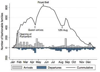
(31) time in the seventeenth century. British peers typically resided in isolated manors on their countryside estates. From February to August, however, they moved to London to attend Parliament. Their whole family accompanied them to enjoy a more eventful lifestyle. Why did such a Season not emerge in continental Europe?12 Continental noblemen were not as rural as British peers. Also, most parliaments in the continent did not meet as regularly as in Britain, so continental aristocracy did not annually migrate to the capital. In addition, primogeniture and entailment allowed the peerage and gentry to remain small enough that these meetings in London were possible. Around 1900, only 1 in 3,200 people in Britain was an aristocrat. In comparison, the proportion in continental Europe was 1 in 100 (Beckett 1986: pp. 35-40). The Season peaked between the 1800s and the 1870s (Ellenberger 1990). During that period, the London Season was a huge event that almost all of the British nobility and gentry attended. Figure 1.2 (Sheppard 1977) plots more than 4,000 movements into and out of London by members of the “fashionable world,” as was reported in the Morning Post in 1841. At the beginning of the year, most people of fashion were out of town. The biggest influx came at the end of January when Parliament convened and anyone who was anyone in the elite moved from their country seats to London. This convergence gave rise to a brief pre-Easter season, marked by numerous dinners and soirées. On April 20, the Queen returned from Windsor, and the first debutante was presented at court, officially entering the marriage market. This marked the commencement of the main Season and was the most crowded time of year in London. Many social events designed to introduce bachelors to debutantes took place. For example, on May 15 — the day of the royal ball at Buckingham — more than 800 “fashionable” families were in London. After a gradual drift away from London, the Season was officially over by August 12, when the shooting season started and most peers moved back to their country estates. This seasonal migration was repeated annually. What was the purpose of the Season? Although in 1841 seasonal mi12. Although Paris and Vienna developed their own marriage markets, they never eclipsed the London Season.. 11.

(32) grations coincided with the Parliamentary calendar, cumulative inflows peaked between Easter and August, when most of the social events crucial to the “matching process” took place. In addition, Sheppard (1977) notes that families that were not prominent in politics, such as the earls of Verulam and Wilton, also showed the same migration pattern, indicating that the Season provided opportunities other than political lobbying.13 The unspoken purpose of these festivities was to bring together the right sort of people, thus “providing the setting for the largest marriage market in the world” (Aiello 2010). The Season became crucial in the nineteenth century, when arranged marriages were no longer acceptable so that individual choice must be carefully regulated to ensure exclusion of undesirable partners É Under such a system it was vital that only potentially suitable people should mix. To meet these ends, balls and dances became the particular place for a girl to be introduced into Society. (Davidoff 1973: p. 49) To restrict the pool of singles, most of the social events in the Season took place in private venues or in the homes of the elite, who carefully selected their guests based on status (Davidoff 1973). Public meeting places like Ranelagh or Hurlingham closed down, and the “fashionable world” put a stop to masked balls, easily gate-crashed by commoners (Ellenberger 1990: p. 636). The expenses required to participate in the Season also selected the most suitable candidates. Renting a house in Grosvenor Square or organizing a ball for hundreds of guests was extremely expensive. Earl Fitzwilliam devoted £3,000 in 1810 solely to entertaining guests. The Duke of Northumberland spent around £20,000 in the Season of 1840 (Sheppard 1971), at a time when a bricklayer could expect to earn 6 shillings (3/10 of a pound) for a 10-hour day (Porter 1998: p. 176). Very few could afford this standard of living. The arrangement 13. One can presume that the Parliamentary motive actually played a secondary role. Parliament sessions were adjourned when the Derby took place. As Harper’s Monthly Magazine stated once, “The Season depends on Parliament, and Parliament depends on sport” (May issue, 1886; quoted in Aiello 2010).. 12.

(33) also excluded impoverished peers who, after generations of gambling or mismanagement, were hard-pressed for money. Participating in the Season, thus, also signaled financial strength. Within the best circles, the race to find a proper husband started with presentation at court and was followed by a whirl of social events. Lucy, daughter of the fourth Baron Lyttelton, kept a diary. She described June 11, 1859 as “a very memorable day” and a “moment of great happiness.”14 She was to be presented to Queen Victoria at court, officially coming out into society. In the following weeks, before returning to Hagley Hall, the family seat in Worcestershire, Lucy attended countless breakfasts, evening parties, concerts, and balls, where she danced with the most eligible bachelors. She even participated in a royal ball at Buckingham Palace, where she thought her heart “would crack with excitement!”15 Lucy’s experience was not unique. Before the start of the Season, the most fortunate 18-year-old girls were presented to the Queen at St. James’s Palace.16 This event, considered the most important day in a woman’s life, symbolized the change in status from childhood to adult life (Davidoff 1973). In practice, it was a public announcement of who was on the marriage market. As reflected in Lucy’s diary, after coming out young ladies began a stressful routine: balls, concerts, breakfast with guests, equestrian events, cricket matches, promenades, tea parties, opera, theater ... During the Season, it was usual for a young lady to start the day with a ride across Hyde Park at 10 am and end up at 3 am the following morning at a ball (Malheiro 1999). Lady Dorothy Nevill remembered than in her first Season she attended “50 balls, 60 parties, 30 dinners and 25 breakfasts” (Nevill 1920). This whirlwind of social events facilitated frequent encounters between singles. In particular, the Royal Academy Summer Exhibition was considered the first round for debutantes, and “ascot races were always the high point of the Season.” They were described as “the 14. The diary of Lady Frederick Cavendish, June 11, 1859. Diary, June 29, 1859. 16 To be eligible, a young lady had to be sponsored by someone who had already been accepted in the royal circle, usually her mother. 15. 13.

(34) Eden of debutantes and the milliners’ harvest” (Harper’s Monthly Magazine, 1886; quoted in Aiello 2010). Meetings at Almack’s were popular, but royal parties were the most exclusive events, giving “a stamp of authority to the whole fabric of Society” (Davidoff 1973: p. 25). Many ladies met their future husbands at these balls, which have been described as “mating” rituals (Inwood 1998). The pressure for these ladies to get married was enormous. They had only two to three Seasons to get engaged to a suitable partner. After that, they were written off as failures. If they “crossed the Rubicon” of 30 years, they became confirmed spinsters (Davidoff 1973: pp. 52, 54). The fate of Georgiana Longestaffe, a lady in her late 20s in Trollope’s The Way We Live Now, illustrates how much a girl’s marriage prospects deteriorated as years went by. Georgiana “had meant, when she first started on her career, to have a lord; but lords are scarce [...] She had long made up her mind that she could do without a lord, but that she must get a commoner of the proper sort [...] But now the men of the right sort never came near her” (Ch. 32). Couples did not have much time to get to know each other. For example, decorum rules prevented a girl from dancing more than three times with one particular partner or sitting out a dance with a young bachelor (Davidoff 1973: p. 49). Unsurprisingly, marriages were not typically love matches but based on money or eligibility. Adultery was consequently commonplace. Oscar Wilde wrote, “I don’t care about the London Season! It is too matrimonial. People are either hunting for husbands, or hiding from them.”17 Davidoff summarizes the materialistic view of marriage by the British aristocracy: Marriage was considered not so much an alliance between the sexes as an important social definition; serious for a man but imperative for a girl. It was part of her duty to enlarge her sphere of influence through marriage. (Davidoff 1973: p. 50) The demise of the Season in the late nineteenth century is inextricably linked with the decline of the British nobility. The immense economic 17. Oscar Wilde, An Ideal Husband (First Act).. 14.

(35) power of this aristocracy rested on a simple foundation: wealth in the form of land. According to Cannadine (1990), protection from foreign competition and light taxes made British agriculture very profitable from the 1840s to the 1870s. However, an agricultural downturn began in the 1870s. Estates that could once support their mortgages — and their proprietors’ opulent lifestyles — fell into ruin. This was reflected in the Season. After the 1870s, many social events became public, and young ladies of commoner or colonial origins began to be presented at court (Ellenberger 1990). It was the death of the Season. Lady Nevill observed that “society, in the old sense of the term, may be said, I think, to have come to an end in the “eighties” of the [nineteenth] century.” (Nevill 1910: p. 51). As Turner (1954) concludes, “love laughed at lineage” (p. 184).. 1.3. Data sources. I use four data sources, two of which are newly computerized, and one of which is based on hand-collected archival documents. To describe the marriage behavior of the British elite, I use the Hollingsworth genealogical data on the British peerage (1964). I complement this dataset with family seats and landholdings from two published sources: Burke’s Heraldic Dictionary (1826) and Bateman’s Great Landowners (1883). Finally, to measure when the Season worked smoothly and when it was disrupted, I construct a new series of attendance at royal parties from the British National Archives.. 1.3.1. Peerage records. The participants in the Season were the royals, peers, old landed gentry, and some successful commoners.18 This well-defined group aroused cu18. British society is divided into classes according to political influence. The head of the society is the Sovereign. The second strand is the peerage, represented in the House of the Lords. In sharp contrast with continental Europe, only the heir inherited the nobility status. This reduced the size of the nobility in Britain. Individuals who were neither peers nor royals were commoners. Again, the term differs from its meaning in. 15.

(36) riosity, which eventually led to the publication of their family histories. Arthur Collins published the first peerage record in 1710. Since then, many genealogic studies have updated his work.19 For the sake of illustration, Figure 1.A1 in the appendix shows the entry for Charles George Lyttelton, brother of Lucy Lyttelton, from Cokayne’s Complete Peerage. Hollingsworth (1964) collected this genealogical material for his study of the British peerage. He tracked all peers who died between 1603 and 1938 (primary universe) and their offspring (secondary universe).20 The data comprises approximately 26,000 individuals. Each entry provides information about spouses’ vital events (date of birth, marriage, and death), social status, whether the husband was heir-apparent at age 15, and the status of the highest ranked parent. Status is presented in five categories: (1) duke, earl, or marquis, (2) baron or viscount, (3) baronet, (4) knight, and (5) commoner. Moreover, the entries state whether a particular title belonged to the English, Scottish, or Irish peerage. Note that the Hollingsworth dataset excludes the landed gentry, who also participated in the Season. The gentry and the peerage, however, did not always attend the same parties; the Season was not a uniform event but consisted of many “layers” (Wilkins 2010: p. 30). In this paper, thus, I focus on the layer for which marriage has the highest stakes — the peerage.. Europe since the landed gentry (baronets and knights) belonged to this class. 19 Three peerage records stand out: Burke’s Peerage and Baronetage, Debrett’s The Peerage of the United Kingdom and Ireland, and Cokayne’s Complete Peerage. The genealogist John Burke wrote Landed Gentry, a similar record for knights and baronets. This last piece tends to be quite mythological, the result of centuries of word-of-mouth information. Oscar Wilde once said, “It is the best thing the English have done in fiction” (Burke’s Family et al. 2005). 20 The primary universe was defined from Cokayne’s Complete Peerage. The universe of children was found from a variety of sources: Collins’ Peerage of England, Lodge’s Peerage of Ireland, Douglas’ Scots Peerage, Burke’s Extinct Peerage and modern peerage editions by Burke and Debrett. The remaining gaps were filled from a large list of sources, among which Burke’s Landed Gentry stands out. See Hollingsworth (1964) for details.. 16.

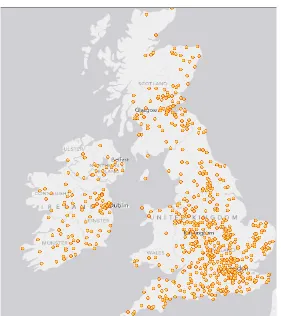
(37) 1.3.2. Family seats. The Hollingsworth dataset is a valuable source of information about marriage and the social position of spouses. Unfortunately, no information regarding birthplace or residence is available. To resolve this, I exploit the fact that each titled family was required to build a seat in their estate and to live there for most of the year.21 Family seats are recorded in heraldic dictionaries. These dictionaries are summarized peerage records that contain additional information at a family level: religious affiliation, motto, coat of arms, and family seats. The most relevant source for my purposes is Burke’s Heraldic Dictionary (1826). Most of the young aristocrats who married between 1851 and 1875 were recorded as presumptive heirs in this source. Therefore, the family seats in Burke’s dictionary correspond in general to the seats where the individuals under analysis grew up and lived most of the year.22 After going through each entry in Burke’s Heraldic Dictionary (1826), I gathered information on 694 country seats for 498 families linked to the peerage. Then, I georeferenced these seats using GeoHack. Figure 1.3 illustrates their geographic distribution, indicating that the nobility was well dispersed all over the British Isles and that seats were quite isolated from each other. Merging this information with the Hollingsworth dataset gives me 351 couples that marryied between 1851 and 1875 for whom both seats are recorded.23 For these individuals, I determine the distance between the 21. On the importance of seats for the British aristocracy, see Stone and Stone (1984). They use ownership of a large house as the criterion for belonging to the elite. 22 Moreover, country seats were expensive to build and representative of long lasting lineages. Therefore, they generally remained in the hands of the same family generationafter-generation until the 1870s, when the aristocracy started its decline. 23 Specifically, I merge the entries in Burke’s dictionary with the individuals in the Hollingsworth dataset, matching own title for males and parental title for women. When parental (own) title of a female (male) is not available, I try to match it using own (parental) title. Moreover, some entries in the Hollingsworth dataset are labeled with two titles, such as James Richard Stanhope, 7th Earl of Stanhope and 13th Earl of Chesterfield. Stanhope is recorded as having grown up in both the Chesterfield and the Stanhope country seats. With this methodology, all but four titles from Burke’s Heraldic Dictio-. 17.

(38) spouses’ seats using Vincenty’s algorithm (Vincenty 1975). When one or both spouses have more than one seat — as was the case for Lord Cavendish — I take the minimum distance. Note that, by construction, distance is only defined when both spouses are peers or peers’ offspring. Henceforth, I restrict the analysis of geographic endogamy to individuals who married within the peerage.. 1.3.3. Bateman’s Great Landowners. In Jane Austen’s Pride and Prejudice, Mr. Darcy is described as a wealthy gentleman with an income exceeding £10,000 a year and proprietor of Pemberley, a large estate in Derbyshire. The wealth and estates owned by nonfictional aristocrats were also public knowledge thanks to Bateman’s The Great Landowners of Great Britain and Ireland (1883). The book consists of a list of all owners of 3,000 acres and upwards by 1876, worth £3,000 a year. Also, 1,300 owners of 2,000 acres and upwards in England, Scotland, Ireland, and Wales are included. Each entry states acreage and gross annual rents. The book also reports the alma mater of the landowner, the clubs to which he belonged, whether he took his seat in Parliament, and other services he provided to the Queen. The years of birth, marriage, and succession are included when known. As an example, the entry for Charles George Lyttelton is shown in the appendix (Figure 1.A2). For the 558 men who appeared both in Bateman’s Great Landowners (1883) and in the Hollingsworth dataset, I created a computerized database of all relevant information. Then, I assessed the family landholdings of their wives. Specifically, I included the landholdings of any of hers close relatives. Using this procedure, I matched 355 wives.24 nary are matched. 24 Seventy-two percent of the matched wives are daughters and sisters of great landowners. Family estates and gross annual rents are similar across family relations. The exception is landowners’ sisters, who belong to families holding larger estates. Table 1.A1 in the appendix summarizes the acreage and gross annual rents of the matched wives by family relation.. 18.

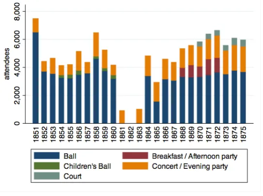
(39) 1.3.4. Lord Chamberlain’s records. Lord Chamberlain’s department at the British National Archives provides data on balls, concerts, and all sorts of parties held at Buckingham or St. James’s Palace during the London Season. Individuals invited to these events are listed in hierarchical order. Absentees are also listed or appear with their names crossed off. The period covered is from 1839 to 1902.25 From Lord Chamberlain’s handwritten invitation lists from 1851 to 1875, I recorded the number of invitations issued, the numbers attending and excused, the type of party, and the date of the event. In total, I recorded 121 parties. Figure 1.4 plots the number of attendees at royal parties over time by type of event. The initial year, 1851, displays unusually high attendance rates, explained by the Crystal Palace Exhibition held in London that year. After that, there seems to be an increasing trend: in the early 1850s balls and concerts were attended by approximately 4,000–5,000 guests. In comparison, on June 24, 1874, a single royal ball brought together almost 2,000 people! The variety of parties also increased, including invitations for breakfast and afternoon parties. Crucially, this evidence reveals a huge disruption to the Season between 1861 and 1863. This was the result of Queen Victoria’s mourning for the death of her husband, Prince Albert. In the empirical analysis, I use this large shock to identify the effects of the Season on marriage outcomes.. 1.4. Empirical analysis. This section presents the empirical results. First I describe marriage outcomes in 1801–75, when the Season was at its peak. I then identify the extent to which these marriage patterns were shaped by the London Season. To do so, I use exogenous variation in attendance to royal parties coming from changes in the size of the marriageable cohort. Finally, I establish a causal link between search frictions and sorting by analyzing 25. The exact references are LC 6/31-55 for the period 1839-76, and LC 6/127-156 for 1877-1902. Additional lists are also provided in LC 6/157-164.. 19.

(40) marriage behavior during the interruption of the Season after the death of Prince Albert (1861–63).. 1.4.1. Data descriptives. From about 1800 to the 1870s, the Season was at its peak (Pullar 1998 and Ellenberger 1990), social parties were crowded, and presentation at court was considered the most important day in a girl’s life (Davidoff 1973). What did marriage outcomes look like during the Season’s golden years? Table 1.1 shows marriage outcomes of all 2,570 peers and peers’ sons marrying between 1801 and 1875. The row variable is the rank of the husband at age 15.26 The column variable is the wife’s social status, measured as the rank of her father. Each cell contains observed percentages at the top, expected percentages if the two variables were independent in italics, and the difference between the two below. For example, 39.3 percent of duke heirs who married during 1801–75, did so with the daughter of a duke. Under random matching, only 17.9 percent of them would have married such an eligible bride. The difference between the two, thus, is 21.4 percentage points. The largest discrepancies are concentrated in two areas. First, peer heirs are much more likely to marry peers’ daughters than under random matching. Second, commoners at age 15 and barons’ sons who are on the lower tail of the social distribution only manage to marry girls of commoner origin. Overall, the relation between the husband and wife’s rank is significant, as indicated by the chi-square test. The gamma test and Kendall’s tau-b indicate that this relation is positive: husbands with a higher social position married the best-ranked spouses and vice versa. In other words, there was positive assortative matching in social status. Table 1.2 shows marriage outcomes from the perspective of peers’ 26. Rank at age 15 allows me to proxy how these individuals appeared in the marriage market. This is particularly important for those individuals who were born commoners, remained commoners at the time of their marriage, but ended their lives holding a peerage — either by creation or by inheriting a distant relative’s title. This individuals compose the “Commoners at 15” category.. 20.

(41) daughters. Between 1801 and 1875, dukes’ daughters married significantly better than barons’ daughters. Under random matching, the latter would have married duke heirs at a larger rate than they actually did. Again, the aggregate statistics confirm that there was positive assortative matching in terms of social class. This suggests that dukes, earls, and marquises looked down not only on commoners, but also on barons and viscounts. Discrimination also existed on the basis of family name, with peers from “old” families marrying much better. Table 1.3 shows that men whose families held land at the time of Henry VIII were 10 percentage points less likely to marry a commoner and 7 percentage points more likely to marry the daughter of a duke than men with a less distinguished pedigree. In nineteenth century Britain, social prestige was not restricted to heraldry. Estate property and gross annual rents from land were also important determinants of one’s position in the social elite.27 Table 1.4 shows marriage outcomes for peers in possession of 2,000 acres and upwards by the 1870s. I cross-tabulate their acreage against the landholdings of their wives’ families. Acreage is divided into six classes following Bateman’s categorization (Bateman 1883: p. 495). As in Table 1.1, each cell contains observed percentages, percentages under random matching in italics, and the difference between the two below. The majority of great lords (64.5 percent) married spouses whose families were listed in Bateman’s Great Landowners (1883). In addition, proprietors of smaller estates (less than 10,000 acres) were more likely to marry outside the circle of great landowners. The aggregate statistics suggest a strong pattern of positive assortative matching in terms of land: hus27. Several great landowners listed in Bateman wrote letters to the author with outrage and demands for the immediate correction of the acres and rents assessed to them. Lord Overstone, for example, complained that “this list is so fearfully incorrect that it is impossible to correct it” (Bateman, p. 348). These complaints might seem unwise in the context of the 1870s, when a the rising public clamor about what was called the “monopoly of land”, was encouraged by some members of the press. The complaints of the British nobility, therefore, cannot but subscribe their view of landholdings as a signal of social position.. 21.

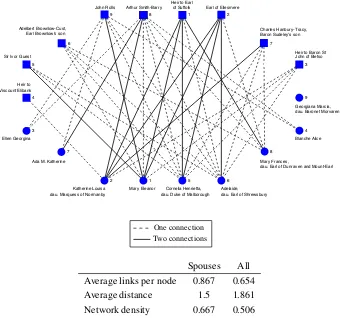
(42) bands in possession of larger estates married spouses from highly accomplished families, and vice versa. Table 1.5 presents the results in terms of rents from land. Again, marriages were not random; richer landowners were more likely to marry spouses from the most endowed families. Positive assortative matching in landholdings is not the result of an arbitrary definition of land classes. Figure 1.A3 in the appendix shows the results of a kernel-weighted local polynomial regression of wife’s landholdings on husband’s landholdings. The advantage of using nonparametric regression is that these techniques allow the data to speak for itself. No assumptions are made about the functional form for the expected value of the wife’s landholdings given husband’s landholdings. Results suggest that both in terms of acreage (left panel) and in terms of land rents (right panel), wealthier individuals were more likely to marry spouses from well-accomplished families. All together, this evidence suggests that the children of the nobility sorted in the marriage market on the basis of socio-economic status. Figure 1.5 illustrates the extent to which individuals bonded with similar others. The network diagram shows the connections between peers in possession of 2,000 acres and upwards marrying in 1862 and their spouses. Specifically, a man and a woman are linked if their fathers had the same social status or if the man and any woman’s relative were in possession of similar amounts of land28 or belonged to the same club. Except for Georgiana Marcia, all individuals were well connected; the fashionable world was a complex, dense network. The average man was connected to more than half of the women. However, the number of connections between spouses was on average higher than between men and women who did not marry (see Table 1.A2 in the appendix for details). This suggests that people’s choice set was somehow limited to those with whom they were most similar. The Season, by pulling singles from all over the country, allowed individuals from very distant places to court. Table 1.6 shows that during the golden age of the Season very few spouses came from geographically ad28. To be precise, the link is established if they belonged to the same “Bateman class”, as depicted in Table 1.4.. 22.