Electromagnetic models for ultrasound image processing

(1)

ADVERTIMENT. La consulta d’aquesta tesi queda condicionada a l’acceptació de les següents condicions d'ús: La difusió d’aquesta tesi per mitjà del servei TDX (www.tesisenxarxa.net) ha estat autoritzada pels titulars dels drets de propietat intel·lectual únicament per a usos privats emmarcats en activitats d’investigació i docència. No s’autoritza la seva reproducció amb finalitats de lucre ni la seva difusió i posada a disposició des d’un lloc aliè al servei TDX. No s’autoritza la presentació del seu contingut en una finestra o marc aliè a TDX (framing). Aquesta reserva de drets afecta tant al resum de presentació de la tesi com als seus continguts. En la utilització o cita de parts de la tesi és obligat indicar el nom de la persona autora.

ADVERTENCIA. La consulta de esta tesis queda condicionada a la aceptación de las siguientes condiciones de uso: La difusión de esta tesis por medio del servicio TDR (www.tesisenred.net) ha sido autorizada por los titulares de los derechos de propiedad intelectual únicamente para usos privados enmarcados en actividades de investigación y docencia. No se autoriza su reproducción con finalidades de lucro ni su difusión y puesta a disposición desde un sitio ajeno al servicio TDR. No se autoriza la presentación de su contenido en una ventana o marco ajeno a TDR (framing). Esta reserva de derechos afecta tanto al resumen de presentación de la tesis como a sus contenidos. En la utilización o cita de partes de la tesis es obligado indicar el nombre de la persona autora.

(2)

P

H

D T

HESIS

Electromagnetic Models for Ultrasound

Image Processing

Author:

Hugo NAVARRETE

Supervisor:

Ramón MUJAL, Ph.D

A thesis submitted in fulfilment of the requirements for the degree of Doctor of Philosophy

in the

Department of Electrical Engineering

(3)

Declaration of Authorship

I, Hugo NAVARRETE, declare that this thesis titled, ’Electromagnetic Models for Ultra-sound Image Processing’ and the work presented in it are my own. I confirm that:

• This work was done wholly or mainly while in candidature for a research degree at this University.

• Where any part of this thesis has previously been submitted for a degree or any other qualification at this University or any other institution, this has been clearly stated.

• Where I have consulted the published work of others, this is always clearly at-tributed.

• Where I have quoted from the work of others, the source is always given. With the exception of such quotations, this thesis is entirely my own work.

• I have acknowledged all main sources of help.

• Where the thesis is based on work done by myself jointly with others, I have made clear exactly what was done by others and what I have contributed myself.

Signed:

Date:

(4)

(5)

“The same equations have the same solutions”

Richard Phillips Feynman

The Feynman Lectures on Physics Vol II

(6)

(7)

Acknowledgements

I am deeply grateful to my advisor Dr. Ramón Mujal-Rosas, PhD for his helpful guidance and unconditional support. To AECI (Agencia Española de Cooperación In-ternacional) and COLCIENCIAS (Departamento Administrativo de Ciencia, Tecnología e Innovación, Colombia) for their financial support in the initial stages of the project. To my friend Dr Alejandro César Frery, PhD who first pointed out the basic ideas of this work. To my brother Dr. Solón Navarrete M.D. for his comments and fruitful dis-cussions. And to My Wife, Mónica: you are part of my life, this could not have been done without your love and support.

(8)

(9)

List of Figures

2.1 Rayleigh Distribution . . . 13

2.2 Rice Distribution Motivation . . . 14

2.3 Rice Distribution . . . 15

2.4 K-distribution . . . 17

2.5 Homodyned K Distributions (ν= 0,0< α <20) . . . 19

2.6 Homodyned K Distributions (ν= 0.5,0< α <20) . . . 20

2.10 Homodyned K Distributions (α= 0.5,0< ν <20) . . . 24

4.1 Montecarlo experiment 1 . . . 46

(14)

6.1 Ultrasound B-scan image filtering. . . 82

6.2 Ultrasound B-scan image segmentation . . . 83

6.3 Ejection Fraction estimation . . . 84

(15)

Dedicated to My Parents María Elvia (in memoriam) and Jesús

Francisco. To My Sisters and Brothers: José "Froidon" (in

memoriam), Carlos Alberto "Lagüete", Carmenza "Mana",

Marcelo "March", Aristóbulo "Lacrija", Marina "Palela",

Clementina "Tina" (in memoriam), Solón "Ranitas", Jairo

"Yaripal", Sandra "Lachanda" and Elkin "Burropín". To My Wife

Mónica. And to my son, Hugo Alberto

(16)

(17)

Abstract

Speckle noise is inherent when coherent illumination is employed because the backscat-tered echoes from the randomly distributed scatterers in the microscopic structure, i.e. under spatial resolution, of the medium are the origin of speckle phenomenon; which characterizes coherent imaging with a granular appearance. It is the case for example of Laser, Synthetic Aperture Radar (SAR), Sonar, Magnetic Resonance, X-ray or Ultra-sound imagery.

Due to its random nature, statistical modeling is of particular relevance when deal-ing with speckled data in order to obtain efficient image processdeal-ing algorithms. It can be shown that speckle noise is of multiplicative nature, strongly correlated and more importantly, with non-Gaussian statistics. These characteristics differ greatly from the traditional assumption of white additive Gaussian noise, often assumed in image seg-mentation, filtering, and in general, image processing; which leads to reduction of the methods effectiveness for final image information extraction; therefore, this kind of noise severely impairs human and machine ability to image interpretation.

Clinical ultrasound imaging systems employ nonlinear signal processing to reduce the dynamic range of the input echo signal to match the smaller dynamic range of the dis-play device and to emphasize objects with weak backscatter. This reduction in dynamic range is normally achieved through a logarithmic amplifier i.e. logarithmic compres-sion, which selectively compresses large input signals. This kind of nonlinear com-pression totally changes the statistics of the input envelope signal; and, a closed form expression for the density function of the logarithmic transformed data is usually hard to derive.

This thesis is concerned with the statistical distributions of the Log-compressed am-plitude signal in coherent imagery, and its main objective was to develop a general statistical model for log-compressed ultrasound B-scan images. The developed model is adapted, making the pertinent physical analogies, from the Multiplicative Model in Synthetic Aperture Radar (SAR) context. It is shown that the proposed model can suc-cessfully describe log-compressed data generated via Montecarlo methods from mod-els proposed in the specialized ultrasound image processing literature. Also, the model is successfully applied to model in-vivo echo-cardiographic (ultrasound) B-scan im-ages.

(18)

2

Necessary theorems are established to account for a rigorous mathematical proof of the validity and generality of the model. Additionally, a physical interpretation of the parameters is given, and the connections between the generalized central limit theo-rem, the multiplicative model and the compound representations approaches for the different models proposed up-to-date, are established. It is also shown that the log-amplifier parameters are included as model parameters and all the model parameters are estimated using moments and maximum likelihood methods. Finally, three ap-plications are developed: speckle noise identification and filtering; segmentation of in vivo echo-cardiographic (ultrasound) B-scan images and a novel approach for heart ejection fraction evaluation.

(19)

Prologue

Motivation

Various models have been introduced in the literature during last forty years for the statistics of ultrasound echo signals. However, when a log-compression or other (non-linear or (non-linear) operators are applied to the echo envelope, the distribution of gray lev-els no longer follows the distributions computed for the RF echo envelope; as a result, computing the Log-compressed data distribution remains as an open problem whose solution should be applied to a wide kind of both theoretical and practical problems, with a high potential for patents generation processes.

Objectives

• The main objective is to develop a general model that includes the known models as particular cases.

• Once the general model is obtained, the objective is apply it to ultrasound B-scan image processing.

Contributions

• A new statistical model for Ultrasound B-scan images is developed.

• It is shown that the new model includes as a particular cases, after Log-compression, most of the models proposed up-to-date .

• The new model parameters include the Log-amplifier parameters, and can be estimated with standard parameter estimation methods.

• The new model is applied successfully to:

– Theoretical random walk and Brownian stochastic process study.

– Speckle noise identification and filtering.

– Ultrasound B-scan image segmentation.

– Heart ejection fraction (EF) evaluation

(20)

4

Thesis outline

• Chapter 1: Introduction

A review of previous and related works, state of the art.

• Chapter 2: Statistical models for Ultrasound RF data

A review of the models proposed up-to-date for RF envelope data is presented. Also, different approaches for study those distributions are presented and re-lated: Central Limit Theorem, Compound Distribution and Multiplicative model approaches.

• Chapter 3: A general model for ultrasound B-scan images

GA0 from SAR image processing is studied and adapted to ultrasound RF enve-lope data. Then, its Log-Compressed version and the physical meaning of model parameters are deduced. Also, model parameters are estimated using moments and maximum likelihood methods.

• Chapter 4: Log-compressed data modeling.

A Montecarlo study is performed with the distributions presented in Chapter 3. Log-compressed data are simulated and then they are modeled with the Model developed in Chapter 4. Finally, goodness of fit tests are performed for null hy-pothesis testing.

• Chapter 5: Central Limit Theorem revisited.

The mathematical theory is presented to demonstrate the model generality. It is shown formally that the developed model has as particular cases all the models presented in chapter 3, after Log-compression.

• Chapter 6: Applications

– Speckle noise filtering in Log-compressed B-scan images.

The new model is applied to speckle noise identification and adaptive filter-ing.

– Log-compressed B-scan images segmentation.

The new model is applied to Log-compressed B-scan images segmentation.

– Hearth ejection fraction (EF) measurement.

The importance of EF estimation is presented and the new model is applied for EF measurement. A comparison study is carried to verify the perfor-mance of the new approach.

• Chapter 7: Conclusions and future work.

(21)

Chapter 1

Introduction

1.1 General Considerations

Speckle noise is inherent to coherent imaging systems because the backscattered echoes from the randomly distributed scatterers in the microscopic structure, i.e. under spatial resolution, of the medium are the origin of speckle phenomenon; which characterizes coherent imaging with a granular appearance. It is the case for example of Laser, Syn-thetic Aperture Radar (SAR), Sonar, Magnetic Resonance, X-ray or Ultrasound imagery. The emitted or interrogating pulse is modeled as a superposition of progressive plane waves; when these waves encounter an interface between two media with dif-ferent wave propagation properties, a part of the incident waves are reflected (specular echoes). Along with these specular echoes, backscattered echoes from the microscopic structure of the medium are added.

Due to its random nature, statistical modeling is of particular relevance when deal-ing with speckled data in order to obtain efficient image processdeal-ing algorithms.Speckle noise is of multiplicative nature, strongly correlated and more importantly, with non-Gaussian statistics. These characteristics differ greatly from the traditional assumption of white additive Gaussian noise, often assumed in image segmentation, filtering, and in general, image processing; which leads to reduction of the methods effectiveness for final image information extraction; therefore, this kind of noise severely impairs human and machine ability to image interpretation. Several distribution families have been proposed for coherent illuminated images. The large variability of models is due to the strong dependence of the observed statistics on the density of scatters and on their spa-tial distribution. Most of the reported models are for describe the envelope of received echo signal; but in the ultrasound case it is necessary to account for particular signal processing transformations. This means, that the proposed distributions are valid be-fore typical transformations like low-pass filtering, interpolation, log-compression and Time-Gain-Compensation; in consequence, they are not longer valid for the ultrasound images acquired under clinical conditions

In this thesis, the various models for the first-order statistics of the echo envelope found in the literature are first presented, based on their representation using the multi-plicative model, the central limit theorem and the compound representation approaches. Then, these models are Log-compressed. This transformation led usually to non-analytical expressions which makes necessary the use of Montecarlo simulation methods in order to study the feasibility of any statistical description of the Log-compressed data.

Another aspect of a statistical distribution is the physical meaning of the model pa-rameters in order to relate its goodness of fit on real data with the properties of the analyzed media. It is the case in problems such as tissue characterization (Shankar et al.,1993; Shankar,2001; Shankar et al.,2001; Oelze, O'Brien, and Zachary,2007; Tsui et al.,2008; Vegas-Sanchez-Ferrero et al.,2012) where estimated parameters themselves

(22)

6 Chapter 1. Introduction

are used for classifying purposes. In such a framework, it is necessary to pay atten-tion to the physical meaning of the distribuatten-tion parameters. For instance, a mixture of sufficiently large number of Gaussian distributions could model the histogram of echo envelope, but the physical meaning of the statistics proportions of such mixtures is not clear because a Gaussian distribution is not (directly) meaningful for the first-order statistics of the echo envelope.

The backscattered echo signal received at the transducer of an ultrasound device can be viewed as the vector sum of the individual signals produced by the scatterers dis-tributed in the medium (Wagner et al.,1983; Wagner, Insana, and Brown, 1987. As a result, the framework leading to a physical interpretation of the statistical distributions parameters assumes that the individual contributions of the scatterers are indepen-dent. When exists a periodicity pattern in the scatterers positions (Wagner et al.,

1983; Wagner, Insana, and Brown,1987), or strong specular reflections, then a coher-ent or deterministic componcoher-ent appears in the received signal, because of a scatterers long-range organization (relative to the wavelength). The power of the coherent com-ponent is called the coherent signal power. The remaining power (from the total signal power) is called the diffuse signal power and corresponds to the diffuse (or random) component, made of a diffuse collection of scatterers.

1.2 Central Limit Theorem Approach

Central Limit Theorem states that the sum of a independent and identically distributed (i.i.d.) random variables with finite variances will tend to normal distribution as the number of variables grows. As a result, the magnitude of a limit random phasor sum with finite mean and variance is Rayleigh distributed. Rayleigh distribution was first introduced in the context of sound propagation in Rayleigh,1880. In ultrasound imag-ing, the Rayleigh distribution corresponds to the distribution of the gray level (also called amplitude) in an unfiltered B-mode image, viewed as the envelope of the radio-frequency (RF) image, in the case of a high effective density of random scatterers with no coherent signal component (Wagner et al.,1983).

The Rice distribution also corresponds to a high effective density of random scatter-ers (the diffuse signal component), but combined with the presence of a coherent signal component of power. Thus, the Rayleigh distribution is the special case of the Rice dis-tribution, with no coherent component. The Rice distribution itself first appeared in the context of wave propagation (Nakagami,1960; 1940; Rice,1945); in ultrasound was applied by Insana,1986; Wagner; 1987 and Tuthill, Sperry, and Parker,1988.

The K-distribution corresponds to a variable (effective) densityαof random scatter-ers, with no coherent signal component and was introduced in ultrasound imaging by Shankar et al.,1993. The parameterαcan be viewed as the number of scatterers per res-olution cell or “density”, multiplied by a coefficient depending on the scanning geom-etry and parameters, and the backscatter coefficient statistics, i.e.“effective” (Jakeman and Pusey,1976and Shankar et al.,1993). The parameterαis also called the scatterer clustering parameter Dutt and Greenleaf,1994. The distribution itself appeared first in Lord, 1954in the context of random walks, and was further studied by Jakeman and Pusey,1976in the context of sea echo.

(23)

Chapter 1. Introduction 7

of random walks viewed as a model of weak scattering. Thus, K-distribution, Rice and Rayleigh are particular and/or limiting cases (namely, the effective densityα of random scatterers is “infinite”) of the Homodyned K-distribution, which may be con-sidered the general model.

A Central Limit Theorem Generalization due to Gnedenko and Kolmogorov (Ho-effding et al.,1955) states that the sum of a number of random variables with a power-law tail (Paretian tail with powerα) distribution (and therefore having infinite vari-ance) will tend to a Alpha-Stable distribution as the number of summands grows. If the exponentα>2 then the sum converges to a stable distribution with stability parameter equal to 2, i.e. a Gaussian distribution. As a result Rayleigh distribution is a special case of the square-root-symmetric stable distribution. In Pereyra and Batatia,2012, Alpha-stable distributions have been applied to statistical image processing of high frequency ultrasound imaging, in order to perform tissue segmentation in ultrasound images of skin. It was established that ultrasound signals backscattered from skin tissues con-verge to a complex Levy Flight random process with non-Gaussian–stable statistics. Based on these results, it was proposed to model the distribution of multiple-tissue ultrasound images as a spatially coherent finite mixture of heavy-tailed Rayleigh dis-tributions i.e. alpha-stable disdis-tributions.

1.3 Compound Representation Approach

One important result of Jakeman and Tough,1987is that the Homodyned K-distribution admits a compound representation, i.e. the distribution can be viewed as the marginal distribution of a model in which the Rice distribution has its diffuse signal power mod-ulated by a gamma distribution with meanµand varianceα. In other words, given the effective density of random scatterers, the model results from the joint probability of the amplitude and the modulating variable w (distributed according to a gamma dis-tribution), and the marginal distribution of the variable A is obtained by integrating the joint probability over the domain of w. In the same manner, the K-distribution is the marginal distribution of a model in which the Rayleigh distribution has its diffuse signal power modulated by a gamma distribution.

Another modeling possibility, introduced in Barakat,1986and further developed in Jakeman and Tough,1987, is equivalent to modulate both the coherent signal compo-nent and the diffuse signal power of the Rice distribution by a gamma distribution giv-ing rise to the generalized K-distribution. This distribution has been used in ultrasound imaging in Eltoft,2006c. However, in Eltoft,2005, the Rician inverse Gaussian distri-bution (RiIG) is introduced, and it corresponds to a model in which both the coherent signal component and the diffuse signal power of a Rice distribution are modulated by an inverse Gaussian (IG) distribution, instead of a gamma distribution.

(24)

8 Chapter 1. Introduction

Three other distributions were introduced in the context of ultrasound imaging. The first one is called the generalized Nakagami distribution (Shankar, 2001) and is ob-tained from the Nakagami distribution by a change of variable. This distribution was also proposed independently in Raju and Srinivasan,2002(in the equivalent form of a generalized gamma distribution). The second other distribution is called the Nakagami-gamma (NG) distribution (Shankar, 2003). That distribution can be viewed as the marginal distribution of a model in which the Rice distribution is approximated by a Nakagami distribution, and in which its total signal power (that would correspond to the total signal power of the Rice distribution) is modulated by a gamma distribution. Equivalently, the corresponding Rice distribution would have both its coherent signal power and its diffuse signal power modulated by the gamma distribution. The third distribution is called the Nakagami-generalized inverse Gaussian (NGIG) distribution (Agrawal and Karmeshu,2007), and it corresponds to a model in which the (approxi-mating) Nakagami distribution has its total signal power modulated by a generalized inverse Gaussian (GIG) distribution instead of a gamma distribution.

1.4 Multiplicative Model Approach

The statistical modeling of Synthetic Aperture Radar (SAR) imagery has provided some of the best tools for the processing and understanding of coherent imaging. Among the statistical approaches the most successful is the multiplicative model. This model of-fers a set of distributions that, with a few parameters, are able to characterize most of SAR data. This model is presented, for instance, in Oliver and Quegan,2004, and ex-tended in Frery et al.,1997. This extension is a general and tractable set of distributions within the multiplicative model, used to describe every kind of SAR return. It was then called a universal model, and its properties are studied in Frery et al.,1999; Mejail et al., 2000; Mejail et al., 2003. The multiplicative model is based on the assumption that the observed random field Z is the result of the product of two independent and unobserved random fields: X and Y . The random field X models the terrain backscat-ter, and thus depends only on the type of area each pixel. The random field Y describes the speckle noise, taking into account that the effective number of looks L (ideally) in-dependent images are averaged in order to reduce the noise. There are various ways of modelling the random fields X, whereas the physics of speckle noise allows the as-sumption of a law for Y. This universal model proposes the distribution to describe the amplitude backscatter X, yielding the GA distribution for the return, and the K-distribution is a particular case of this model; while in Eltoft,2006athe Generalized-K and Homodyned-K distributions can be represented as a convolution of these models, i.e. a scale mixture of Gaussians models.

1.5 Logarithmic compression

(25)

Chapter 1. Introduction 9

before, operators other than log-compression can be applied on the envelope. In Navar-rete et al.,2002the Multiplicative model was applied to in vivo B-scan images filtering; and in Nillesen et al.,2008, a linear filter was applied to the RF data before computing the envelope. Five distributions were tested to fit the data: the Rayleigh distribution, the K-distribution, the Nakagami distribution, the inverse Gaussian distribution and the gamma distribution. The authors showed, based on empirical tests that the gamma distribution best fit the data, although the physical meaning for the parameters was not established.

(26)

(27)

Chapter 2

Statistical Models for Ultrasound RF

data

As stated previously, speckle noise is a inherent phenomenon present when coherent illumination is employed, as is the case of sonar, laser, ultrasound, Magnetic Reso-nance, X ray or and synthetic aperture radar (SAR) imagery; therefore, any statistical description of data from these areas can be adapted to the others taking care of the parameters physical meaning in each case. Also, it is necessary to take into account that when the product of the wave number with the mean size of the scatterers is much smaller than the wavelength, and the acoustic impedance of the scatterers is close to the impedance of the embedding medium, a high density of scatterers results in a packing organization that implies a correlation between the individual signals produced by the scatterers (Hawley, Kays, and Twersky, 1967; Twerskyt,1975; 1978, 1987, 1988; Lucas and Twersky, 1987; Berger, 1991) Apart from that case, the backscattered echo signal received at the transducer of an ultrasound device is viewed as a random phasor sum of the individual signals produced by the scatterers distributed in the medium (Wag-ner et al., 1983; 1987). Therefore, statistical description of the envelope signal can be viewed as a statistical description of a random walk in the complex plane.

In this chapter, based on the two excellent reviews by Destrempes and Cloutier,2010

and Mamou and Oelze,2013chapter 10, a review of the models proposed up-to-date for RF envelope data is presented. Also, different approaches for study those distribu-tions are presented and related: Central Limit Theorems, Compound Distribution and Multiplicative model approaches.

2.1 Central Limit Theorem Approach

2.1.1 Rayleigh distribution

Consider a random walk in the complex plane:

A= N

X

j=1

aj (2.1)

Ais the resultant phasor after N steps. The Central Limit Theorem states that when N tends to infinity and the following conditions are met:

• Random phasorsajare independent i.e. uncorrelated.

• Phase and amplitude are independent.

• Phase is uniform distributed.

(28)

12 Chapter 2. Statistical Models for Ultrasound RF data

• Phasor amplitudes are independent and identically distributed, with meanµand varianceσfinite.

Then in the random walk of equation2.1, the join distribution of the uncorrelated real

Arand imaginaryAiparts of the random phasorAwill be Gaussian with no correlation

terms:

P(Ar, Ai) = 1 2πσ2exp

−A

2 r+A2i

2σ2

(2.2)

The envelope signal is the magnitude of resultant complex phasor:

X=

q A2

r+A2i (2.3)

Whose join density in polar coordinates can be expressed as:

Px(X, θ) =

X

2πσ2exp

−X

2

2σ2

(2.4)

As a result, the Amplitude probability density function is the marginal density:

Px(X) =

Z π

−π

Px(X, θ)dθ=

Z π

−π

X

2πσ2exp

−X

2

2σ2

dθ

Px(X) =

X σ2exp

−X

2

2σ2

(2.5)

This distribution function is known as a Rayleigh distribution function, and it is depicted in figure2.1. The parameter

σ2 = ¯a 2

2

where¯a2is the mean intensity of the random stepaj before scaling by the factor√1_N.

After normalizing the contribution of N independent scatterers by the factor √1

N, one

also obtains¯a2 as the mean intensity (in fact, before or after taking the limit asN → ∞

). The idea behind the normalization factor of√1

N (instead of 1/N) is to average out the

intensity of the scatterers (rather than their amplitude), to preserve the mean intensity. In the case of the Rayleigh distribution, the mean intensity (i.e.,2σ2) can be interpreted as the diffuse signal power, because there is no coherent component in the signal.

2.1.2 Rice distribution

Consider a random walk, obtained by adding a constant phasorνto the random walk of equation2.1(see fig. 2.2) which may arise due to periodically located scatterers or due to strong specular scattering:

A=ν + N

X

j=1

(29)

Chapter 2. Statistical Models for Ultrasound RF data 13

FIGURE2.1: Rayleigh Probability Density Function (A) and Cumulative Distribution Function (B)

by Krishnavedala Own work. Licensed under CC0 via Commons

https://commons.wikimedia.org/wiki/File:Rayleigh_

(30)

FIGURE2.2: In the 2D plane, Rice distribution arises by picking a fixed point at distanceν from the origin. Generate a distribution of 2D points centered around that point, where the x and y coordinates are chosen independently from a gaussian distribution with standard deviationσ

(blue region). If R is the distance from these points to the origin, then R has a Rice distribution.

by Sbyrnes321 Own work. Licensed under CC0 via Commons

(31)

FIGURE2.3: Rice Probability Density distribution (up) and its Cumula-tive Distribution Function (bottom)

Licensed under CC BYSA 3.0 via Commons

(32)

The join density function of real and imaginary parts ofAcan now be written as:

P(Ar, Ai) = 1 2πσ2exp

−(Ar+νr)

2_{+ (}_A

i+νr)2 2σ2

(2.7)

The marginal density, can be expressed as (see Jakeman and Tough,1987):

Px(X) =

X σ2exp

−X

2₊_ν2 2σ2

Io νX σ2 (2.8)

Io(x) denotes the modified Bessel function of the first kind of order o (the intensity I should not be confused with the Bessel function Io). Figure2.3shows the Rice probabil-ity densprobabil-ity function and its correspondent cumulative distribution function for differ-ent conditions of coherdiffer-ent compondiffer-ent (ν) and fixed (σ). The figure illustrates that the Rice distribution approaches to Rayleigh distribution when de ratio of the coherent to diffuse (r= _σν) power signals tends to 0; and whenrtends to infinite, Rice distributions becomes a Gaussian Distribution.

2.1.3 K-Distribution

Consider the random walk described by equation 2.1, with independent phase and amplitude, and a uniformly distributed phase, in which the number of steps is variable. Namely, givenαeffective scatters per resolution cell and assuming that the number of steps N follows a negative binomial distribution of meanN¯ so thatp = 1

(1+ ¯N /α). Let

the random step be scaled by the factor1/

√ ¯

N; then, the following random process is obtained:

N ∼N egBin α,1/ 1 + ¯N /α

A|N ∼ √1 ¯ N N X j=1 aj (2.9)

Let N¯ tend to infinite in the random process of equation2.9; then, the amplitude probability density function is a K-distribution (Jakeman and Tough,1987):

P(X) = 4X α

(2σ2₎(α+1)/2Kα−1

r

2

σ2X

!

, α, σ, X >0 (2.10)

Kρis the modified Bessel function of second kind and orderρ. The scale parameter

σ2 = ¯a2/(2α) (2.11)

(33)

FIGURE 2.4: Probability Density K-Distributions (up) and its

Cumula-tive Distribution Function (bottom). For differentαvalues, scale param-eter is adjusted for unitary mean. Rayleigh distribution with unitary mean is plotted as reference. Note that forα >20K-distribution can be

(34)

2.1.4 Homodyned K-Distribution

Homodyned K-Distribution results from adding a coherent signalνto the random pro-cess described by equation2.9,

N ∼N egBin α,1/ 1 + ¯N /α

A|N ∼ν+√1 ¯ N N X j=1 aj (2.12)

Let N¯ tend to infinite in the random process of equation 2.12; then, the ampli-tude probability density function is a Homodyned K-distribution (Jakeman and Tough,

1987):

P(X|σ2, ν, α) =X

Z _{uJ o}₍_uν₎_{J o}₍_uX₎

1 +u2₂σ2

α , α, σ, X >0; ν ≥0 (2.13)

Jo denotes the Bessel Function of the First Kind and order 0; and scale parameter

σ2 = ¯a2/(2α) (2.14)

Homodyned-K distribution has no analytical expression, but can be represented in power series (see Dutt, 1995). Also, note that the Homodyned-K distribution when

ν=0 is the K-distribution and it is shown in Jakeman and Tough, 1987that the limit distribution asα→ ∞is the Rice distribution.

2.2 Compound representation approach

Using characteristic function Jakeman and Tough, 1987 showed that random walks in n dimensions can be described using a compound representation or, equivalently, by the multiplicative model. In this section different proposals using the compound representation are presented.

2.2.1 Homodyned K-Distribution

Equation2.15bellow is the Homodyned-K distribution compound representation (see Jakeman and Tough,1987):

P(X|σ2, ν, α) =

Z ∞

0

Pr(X|ν, σ2w)Pγ(w|α,1)dw, α, σ, X >0; ν ≥0 (2.15)

Pr is the Rice distribution with coherent componentν and variance wσ2; andPγ is

the Gamma Distribution with mean and variance equal toα; therefore, Homodyned-K distribution can be understood as a Rice distribution whose variance is a gamma-distributed random variable. This compound representation led to following limiting distributions:

• K- Distribution givenν →0.

• Rice Distribution asα → ∞

(35)

FIGURE 2.5: Homodyned K-distributions resulting of compounding a modulated Rayleigh (ν = 0) with different effective scatter densities

(36)

FIGURE 2.6: Homodyned K-distributions resulting of compounding a modulated Rice (ν = 0.5) with different effective scatter densities (0.5≤

(37)

(38)

(39)

(40)

FIGURE 2.10: Homodyned K-distributions resulting of compounding different modulated Rice (0.5 ≤ ν ≤ 20) distributions with very low

(41)

FIGURE 2.11: Homodyned K-distributions resulting of compounding different modulated Rice (0.5 ≤ ν ≤ 20) distributions with low

(42)

FIGURE 2.12: Homodyned K-distributions resulting of compounding different modulated Rice (0.5 ≤ ν ≤ 20) distributions with α = 2.0

(43)

(44)

(45)

FIGURE 2.15: Homodyned K-distributions resulting of compounding different modulated Rice (0.5 ≤ ν ≤ 20) distributions withα = 16.0

(46)

Homodyded-K distributions are depicted in figures2.5to2.8, for different parameters condition.

2.2.2 Generalized K-Distribution

From Jakeman and Tough, 1987 (equations 4.10 to 4.12) and used in ultrasound by Eltoft,2006cthe compound representation of the generalized K-distribution is

P(X|σ2, ν, α) =

Z ∞

0

Pr(X|νw, σ2w)Pγ(w|α,1)dw, α, σ, X >0; ν≥0 (2.16)

wherePrdenotes the Rice distribution andPγis the Gamma Distribution with mean

and variance equal toα. Thus, as opposed to the Homodyned K-distribution, both the coherent signal component and the diffuse signal power of the Rice distribution are modulated by a gamma distribution in Generalized-K distribution compound repre-sentation.

2.2.3 Rician Inverse Gaussian Distribution (RiIG)

From Eltoft,2006bthe compound representation of the Rician Inverse Gaussian Distri-bution (RiIG) is

PRiIG(X|νσ2, α) =

Z ∞

0

Pr(X|νw, σ2w)IG(w|

√

λ, λ)dw, λ, σ, X >0; ν ≥0 (2.17)

wherePrdenotes the Rice distribution andIG(w|

√

λ, λ)is Inverse Gaussian Distri-bution, with meanµand shape parameter equal toλ:

IG(w|√λ, λ) =

r λ

2πw3exp(−

λ(w−µ)2

2µ2_w ) (2.18)

The mean and variance ofIG(w|√λ, λ)are both equal to √λ. So, in the compound representation context, √λplays the same role asα in the Gamma Distribution with mean and variance equal toα, however a parameter physical interpretation is not as straight forward.

2.3 Multiplicative model approach

(47)

important exceptions.

Common distributional hypothesis for one-look return data and homogeneous tar-gets are the Exponential and Rayleigh distributions, for intensity and amplitude de-tections, respectively. When the observed region cannot be assumed as homogeneous, other distributions are considered; among these, the K-distributions have received a great deal of attention in the literature, and in chapter 3 a generalization will be ex-posed in detail.

2.3.1 Generalized K-Distribution

From Eltoft,2006ca normal variance-mean mixture model, was presented. An equiv-alent 1-D Gamma variance-mean mixture model is in its most general form expressed as:

Y = (m+bZ+Z1/2X) m, b≥0 (2.19)

Z1/2_{is a square root gamma distribution (i.e. Nakagami distribution) with parameters}

(1,1) equivalent to a Rayleigh distribution; and X is an independent square root gamma distribution with parameters (α, γ>0). This mixture model has as particular cases:

• Rayleigh distribution: m,b=0,α→ ∞.

• K- Distribution: m,b=0.

• Rice Distribution: b=0,α→ ∞.

• Homodyned-k distribution: b=0.

(48)

(49)

Chapter 3

A general model for ultrasound

B-scan images

3.1 Statistical models for SAR data

Among the frameworks for Synthetic Aperture Radar (SAR) image modelling and anal-ysis, the multiplicative model is very accurate and successful. It is based on the as-sumption that the observed random field is the result of the product of two indepen-dent and unobserved random fields: X and Y. The random field X models the terrain backscatter and, thus, depends only on the type of area to which each pixel belongs to. The random field Y takes into account that SAR images are the result of a coherent imaging system that produces the speckle noise, and that they are generated by per-forming an average over statistically independent images (looks) in different bands or polarizations, in order to reduce the speckle noise effect. There are various ways of modelling the random field X; while, with the usual Rayleigh distribution for the am-plitude speckle, resulted in a different distribution families for the return. The distribu-tion parameters depend on the reflective surface (ground in SAR data), and the number of looks. The advantage of the multiplicative model is that it can model extremely het-erogeneous areas like cities, as well as moderately hethet-erogeneous areas like forests and homogeneous areas like pastures. In this chapter, the successful multiplicative model will be adapted from SAR to ultrasound images. Then, the adapted distribution will be Log-compressed and the resulting model parameters will be estimated.

3.1.1 Speckle Noise Model

The speckle noise model, proposed by Arsenault Arsenault and April,1976, is deduced from the coherent imaging mechanism of a SAR system. Under the ideal circumstances the imaged scene has a constant Radar Cross Section (RCS) (i.e., speckle is fully de-veloped and homogeneous surfaces appear as stationary fields).The deducing process based on the coherent imaging mechanism begins with the six reasonable hypotheses as follows (Oliver and Quegan,2004; Moser, Zerubia, and Serpico,2006; Kuruoglu and Zerubia,2004; Goodman,1976):

• Each resolution cell contains sufficient scatterers.

• The echoes of these scatterers are independently identically distributed;

• The amplitude and phase of the echo of each scatterer are statistically indepen-dent random variables.

• The phase of the echo of each scatterer is uniformly distributed in the closed interval [−π, π].

(50)

34 Chapter 3. A general model for ultrasound B-scan images

• Inside a resolution cell, there are no dominant scatterers.

• The size of a resolution cell is large enough, compared with the size of a scatterer.

Secondly, with the six hypotheses mentioned above and the central limit theorem, it can be proven that the energy of each resolution cell has a negative exponential distribution with the mean value equal to the real RCS value of the resolution cell. Finally, according to the hypothesis of constant RCS background, each resolution cell can be considered as a stochastic process, with the ergodic property (i.e., each resolution cell is statistically independent). Therefore, the whole image has a distribution identical to that of a single resolution cell.

3.1.2 The Multiplicative Model

Motivated by the speckle model, Ward Ward,1981proposed the Multiplicative Model of SAR images. The Multiplicative Model combines an underlying RCS componentσ

with an uncorrelated multiplicative speckle componentn, so the observed intensity I in a SAR image can be expressed as the product (Tur, Chin, and Goodman,1982, Xie, Pierce, and Ulaby,2002):

I =σ·n (3.1)

The speckle model is taken as the special example of the Multiplicative Model with a constant RCS (σ). Because the Multiplicative Model is correlated with the underlying terrain RCS (σ), it is usually applied to the intensity data (energy or the square of am-plitude). That is, I in Equation3.1represents the observed value of the intensity. The Multiplicative Model simplifies the analysis of the statistical model of SAR images. So it is widely used to develop models which take the RCS fluctuations into consideration, whereP(σ)represents the RCS component distribution andP(I|σ) is correlated with the distribution of speckle component.

Since the speckle component has a determinate statistical distribution, only the RCS fluctuation component need to be considered when developing the statistical models of SAR images, as a result according3.1, the PDF of the observed intensity is given by:

P(I) =

Z

P(σ)·P(I |σ)dσ (3.2)

The RCS of a homogeneous region (e.g., the grassland region) in either low-resolution or high-resolution SAR images can be expected to correspond to a constant. Actually, most scenes contain in-homogeneous regions with RCS fluctuations (Oliver and Que-gan,2004; Kuruoglu and Zerubia,2004; Moser, Zerubia, and Serpico,2006). According to Jakeman and Pusey, 1976investigations, when the number of scatterers in a reso-lution cell becomes a random variable due to fading phenomenon and the population of scatterers to be controlled by a birth-death-migration process, it should have a Pois-son distribution Oliver and Quegan, 2004 and the mean of the Poisson distribution in each resolution cell (i.e., the expected number of scatterers) itself is also a random variable. If the mean is Gamma distributed, the corresponding intensity data should have a K distribution. Further research indicates that K distribution can be viewed as the combination of two split parts according to Equation3.2 in the framework of the Multiplicative Model (Oliver and Quegan,2004):

(51)

Chapter 3. A general model for ultrasound B-scan images 35

• the Gamma distributed intensity RCS fluctuations.

The K distribution is deduced with the assumption that the underlying intensity RCS fluctuations have a Gamma distribution in a heterogeneous region. The Gamma distri-bution can well describe the characteristics of the RCS fluctuations of a heterogeneous terrain in high-resolution SAR images. The deduced K distribution itself has the mul-tiplicative fading statistical characteristics and usually provides a good fit to the het-erogeneous terrain. Therefore, the K distribution has become one of the most widely used and the most famous statistical models. Furthermore, according to the deducing process of the K distribution, the homogeneous region with a constant RCS can also be described as a special case of the K distribution (Oliver and Quegan,2004). However, K-distributions cannot meet the demand for the statistical modeling of complex scenes in high-resolution images. The complexity of the high-resolution scenes mainly lies in two aspects (Kuruoglu and Zerubia,2004):

• The terrain of the scene is usually extremely heterogeneous, such as the urban region containing many buildings, which results in the severe long-tailed part of the image histogram.

• There exist two or more heterogeneous components in a certain scene, such as a combination of woodlands and grasslands, etc.

To solve these problems, Frery et al.,1997deduced a new statistical model, the GA model, based on the product model assuming a Gamma distribution for the speckle component of multi-look SAR images and a generalized inverse Gaussian (GIG) law for the signal component. It was Frery who first proposed to divide a region as mogeneous, commonly heterogeneous or extremely heterogeneous according to its ho-mogeneous degree when deducing the GA model. The K and G0 (also called B distri-bution) distributions are two special forms of the G model. The former is appropriate for the heterogeneous region and the latter is appropriate for the extremely heteroge-neous region. The G0 distribution can be converted into the Beta-Prime distribution under the single-look condition. Although the G0 distribution is a specific example of the G model, it has a more compact form in comparison with the G model and conse-quently has a simple parameter estimation method. The relationship between the G0 distribution and the K distribution cannot be deduced theoretically, but has been eval-uated via Montecarlo Simulation Methods(Mejail et al., 2001). The parameters of the G0 distribution are sensitive to the homogeneous degree of a region, which makes the G0 model appropriate for modeling either heterogeneous or extremely heterogeneous region. Moreover, moments method can be easily and successfully applied to parame-ter estimation of the G0 distribution; and the Log-Compressed G0 distribution, namely HG0 distribution, has an analytical expression. Also, Frery et al.,1997and Muller and Pac, 1999 carried out experiments on many SAR images of different kinds of terrain with various band, polarization, resolution and look numbers, such as different urban areas, homogeneous and heterogeneous regions, etc. Their results testified the good characteristics of the G0 distribution. In next sections the GA and GA0 models will be presented and adapted to ultrasound B-scan images modeling.

3.2 G

Aistributions for SAR images

Equation3.1can be rewritten in equivalent form:

(52)

Equation3.3 states that the intensity observed value I is the outcome of a random variable defined by the product of two independent random variables: X modeling the terrain backscatter, and Y modeling the speckle noise. In a general situation when independent bands or polarizations images are averaged to reduce speckle noise, it is necessary to take into account the number of looksn; then multi-look intensity speckle appears by taking an average overnindependent samples, leading, thus to a Gamma distribution denoted asYI ∼Γ(n, n)and characterized by the density:

fYI(y) =

nn

Γ(n)y

n−1_exp₍₋_ny₎_{, y, n >}₀

Multi-look amplitude speckle results from taking the square root of the multi-look intensity speckle and, therefore, has a square root of Gamma distribution, denoted as

YA∼Γ1/2(n, n)and characterized by the density:

fYA(y) =

2nn

Γ(n)y

2n−1_exp₍₋_ny2₎_{, y, n >}₀

Though the number of looks should, in principle, be an integer, seldom this is the case when this quantity is estimated from real data due to, among other reasons, the fact that the mean is taken over correlated observations. Therefore, the equivalent num-ber of looks must be estimated (see for example Anfinsen, Doulgeris, and Eltoft,2008).

Frery et al., 1997 proposed modeling amplitude backscatter with the Square Root Generalized Inverse Gaussian Law, i.e.XA∼N−1/2(α, γ, λ), with density given by

fXA(X) =

(λ/γ)α/2

Kα 2

√

λ γx

2α−1_exp₋γ

x2 −λx 2

whereKαdenotes the modified Bessel function of the second kind and orderα. The

parameters space is given by

 



γ >0, λ≥0, if α <0

γ >0, λ >0, if α= 0

γ≥0, λ >0, if α >0

(3.4)

The amplitude return,GA(α, γ, λ), that arises from the product of XA·YA = ZA ∼

GA(α, γ, λ), whereXA ∼ N−1/2(α, γ, λ)and YA ∼ Γ1/2(n, n); is characterized by the

density

fZA(x) =

2nn(λ/γ)α/2 Γ(n)Kα(2

√

λγ)x 2n−1

γ+nx2 λ

(α−n)/2 Kα−n

2pλ(γ+nx2₎ _(3.5)

and parameters space given in equation3.4.

From N−1/2, the Square Root Gamma Distribution (Γ1/2(x, α, λ)) arises by letting

γ →0whileα, γ >0. This distribution is characterized by the density

fXA(x) =

2λα

Γ(α)x

2α−1_exp₍₋_λx2₎_{, α, λ, x >}₀

(53)

fXA(x) =

2

γα_Γ(_α₎x

−(2α+1)_exp₍₋_γ/x2₎_{, α, λ, x >}₀

It should be noticed that, ifX∼Γ1/2(x, η, γ), thenZ = 1/X∼Γ−1/2(z, α, γ−1)with

α=η.

Therefore,Γ1/2(αm, λm)andΓ−1/2(αm, γm)distributions are particular cases ofN−1/2(α, γ, λ)

distribution; and also, using characteristic functions it can be proved that a sequence of random variables obeyingΓ1/2(αm, λm)distributions converges in probability to the

constantβ₁1/2, ifαm, λm→ ∞such thatα/λ→β1when m→ ∞.

As a result, a sequence of random variables obeyingΓ−1/2(αm, γm)distributions

con-verges in probability to the constantβ₂−1/2, ifαm, γm→ ∞such thatα/γ →β2when m

→ ∞.

In this manner, constant amplitude backscatter, used to model homogeneous areas, arises in two situations and are particular cases of the square root of generalized In-verse Gaussian Distribution (GiG).

3.2.1 KA-distribution for SAR image

The K-distribution amplitude return,KA(α, λ), that arises from the product ofXA·YA=

ZA ∼ KA(α, λ), whereXA ∼ Γ1/2(α, λ) andYA ∼ Γ1/2(n, n); is characterized by the

density

fZA(x) =

4λnx

Γ(n)Γ(α)(λnx

2₎(α+n)/2−1_K α−n

2x

√

λn

(3.6)

3.2.2 GA0 distribution for SAR image

GA0 distribution, GA0(α, γ), arises from the product of XA·YA = ZA ∼ GA0(α, γ),

whereXA∼Γ−1/2(α, γ)andYA∼Γ1/2(n, n); is characterized by the density

fZA(x) =

2nnΓ(α+n)γαx2n−1

(54)

3.3 G0 distribution for ultrasound image processing

Acoustical waves are longitudinal, therefore cannot be polarized. Also, ultrasound images are single look i.e. effective number of looks is just n=1; then, amplitude return A=XY is distributed as (Springer,1979):

G0(A) =

Z +∞

−∞

(1/X)fx(X)fy(A/X)dX

With X distributed as:

fx(x) = Γ1/2(x,1,1) = 2xexp(−x2), x >0

and Y with density

fy(y) = Γ−1/2(y, α, γ) =

2γαexp(−γ/y2)

Γ(α)y2a+1 , y, α, γ >0

Therefore G0(A) can be written as:

G0(A) =

Z +∞

−∞

(1/x) 2xexp(−x2)

2γαexp(−γx2/A2) Γ(α)(A/x)2a+1

dx

G0(A) = 2∗2∗γ α

Γ(α)A2α+1

Z +∞

−∞

(x2a+1) exp(−x2(1 + γ

A2))dx

Replacing:

u=x2_{(1 +} γ

A2), x 2₌_u

A2 A2₊_γ

, 2xdx=du

A2 A2₊_γ

,

We obtain:

G0(A) = 2γ α

1 + γ

A2

α+1

Γ(α)A2α+1

Using the Gamma Function definition:

Z +∞

0

uαexp(−u)du= Γ(α+ 1) =αΓ(α)

G0 distribution is obtained:

G0(A, α, γ) = 2α(A/γ)

[1 + (A2_/γ_)]α+1, α, γ, A >0 (3.8)

Here, the random variable A (detected amplitude) results from the product of the random variables xn and ye.Subindex nrepresents the speckle noise, while e is the

(55)

3.4 HG0 distribution for Log-compressed B-scan images

Clinical ultrasound imaging systems employ nonlinear signal processing to reduce the dynamic range of the input echo signal to match the smaller dynamic range of the dis-play device and to emphasize objects with weak backscatter. Typically, the input image could have dynamic ranges of the order of 50-70 dB whereas a display device would have dynamic range of the order of 20-30 dB. This reduction in dynamic range is nor-mally achieved through a logarithmic compression which selectively compresses large input signals.

This kind of nonlinear compression totally changes the statistics of the input enve-lope signal. A closed form expression for the density function of the log transformed distributed data usually is hard to derive. However, it is possible to obtain the density function of log-compressed G0 density function, as will be shown in this section.

3.4.1 Logarithmic Compression Model

The logarithmic compression transfer function can be written as

X=D·ln(A) +G (3.9)

where A is the input to the compression block and X is the output of the compres-sion block. D is a parameter of the compressor which represents the dynamic range of input, and G is the linear gain of the compressor. Here it is assumed that the input is nonzero.

The linear gain parameter, G, does not affect the statistics of the output signal be-cause it just changes the mean of the distribution function. But the dynamic range parameter, D, scales the output signal and is thus important to estimate if one has to invert this logarithmic transfer function.

If the minimum and maximum input values Amin and Amax, are mapped to mini-mum and maximini-mum output values Xmin and Xmax by this logarithmic compression, then the relationship between them can be written as

Xmax =D·ln(Amax) +G

Xmin =D·ln(Amin) +G

Therefore

D= (Xmax−Xmin)/ln(Amax/Amin)

(56)

These are the optimum logarithmic amplifier parameters, D and G, when the input-output dynamic ranges are known. For gray level displays,Xmin = 0andXmax = 255; and a typical input dynamic range,Amin = 0.1mV,Amax= 10V; result in opti-mum logarithmic amplifier parameters ofD= 22.15andG= 204.

3.4.2 A New Statistical Model of Log-compressed B-scan images

When the non-linear transformz=D·ln(A) +Gis applied to Amplitude Distribution

fA, it is transformed as:

fz(z) = (1/D) exp(

z−G

D )fA(exp( z−G

D ))

The new random variable z when fAis a Go distribution, is distributed as:

fz(z) = α        exp z−G

D/2 γ        D 2        1+ exp z−G

D/2 γ        α+1

Replacingd=D/2andexp(−g) =exp(− G

D/2)/γ, HG0 distribution is obtained:

HGo(z) =

αexp((z−g)/d)

d(1 + exp((z−g)/d))α+1, α, g, d >0 (3.10)

It is straight forward to show that the HG0 cumulative distribution function can be expressed as:

FHG0(z|α, d, g) = 1−

1

[1 + exp((z−g)/d)]α, α, d, g >0 (3.11)

(57)

3.5 Moments generating function method for HG0 parameter

estimation

Moments generating function is defined as the expected value ofexp(tX), ifX∼PX(x)

mX(t) =hexp(tX)i=

R

Sexp(tX)PX(x)dx

integration over sample space S; for HG0 distribution, it means:

mX(t) =hexp(tz)i= α_d

R

∞

−∞

exp(tz) exp(z−g d )

[1+exp(z−g d )]

α+1

The moments generating function is (see Appendix A for details)

mX(t) =

exp(gt)

Γ(α) Γ(1 +td)Γ(α−td) (3.12)

and the normalized central moments can be expressed as:

 



µ1 =g−d(ψ(0)(1)−ψ(0)(α))

µ2 =d2(ψ(1)(1) +ψ(1)(α))

µ3 =d3(ψ(2)(1)−ψ(2)(α))

(3.13)

whereψ(n)(x)is the poly-gamma function. From second and third normalized cen-tral moments,αis the solution of the non-linear equation

µ3

µ3/2₂ =µ3 =

(ψ(2)(1)−ψ(2)(α))

(ψ(1)_{(1) +}_ψ(1)₍_α₎₎3/2 (3.14)

Equation 3.14can be solved with standard numerical methods. Parameters (d,g), knowingα, can be expressed easily,

d= (ψ(1)(1) +ψ(1)(α))−1/2

(58)

3.6 Maximum likelihood method for HG0 parameter

estima-tion

From equation3.10the optimization function can be expressed as

LHGo =

X

ln(α) + (z−g)/d−ln(d)−(α+ 1) ln (1 + exp((z−g)/d)) (3.16)

And the maximum conditions, are the partial derivatives of equation3.16with re-spect to the distribution parameters

                         ∂L

∂α = 0 = 1− α N

X

i

ln [1 + exp((z−g)/d)]

∂L

∂g = 0 = 1 +

(α+ 1)

N X

i

exp((z−g)/d) (1 + exp((z−g)/d))

∂L

∂d = 0 = 1−

(α+ 1)

d·N X

i

d·z.exp((z−g)/d) (1 + exp((z−g)/d)) −z/d¯

(3.17)

(59)

Chapter 4

Log-compressed data modeling

A Montecarlo study is performed with the distributions presented in Chapter 2. Log-compressed data are simulated and then they are modeled with the new model de-veloped in Chapter 3. Finally, goodness of fit tests are performed for null hypothesis testing.

4.1 Montecarlo simulation of Log-compressed data

Rayleigh, Rice and K distributions are particular cases of the Homodyned-K and sta-ble distributions, therefore this study will be focused in modeling Log-compressed Homodyned-K and stable distributed data.

4.2 Homodyned-K distributed data simulation

Simulating Homodyned-K distributed data can be done by using the compound rep-resentation (See chapter 2).

P(X|σ2, ν, α) =

Z ∞

0

Pr(X|ν, σ2w)Pγ(w|α,1)dw, α, σ, X >0; ν ≥0 (4.1)

Given parameters (ν,α) i.e. coherent componentν and effective scatterers densityα, the algorithm to generate an lengthN- arrayAof Homodyned-K distributed data, can be expressed as:

• for i= 1 to N

– Generateσnumber using Gamma distribution with parameters (α, 1)

– GenerateA(i)number using Rician distribution with parameters (ν,α)

• next i

(60)

44 Chapter 4. Log-compressed data modeling

4.3 Stable process simulation

Simulating stable distributions can be done with open source code (See appendix C). Then, the algorithm for stable process simulation can be stated:

• for i= 1 to N

– Generate complex Z random variable with X real and Y imaginary stable variables with parameters (α, 1): Z= X + iY.

– Generate random complexηwith magnitudeν

– Stable process is the magnitude of the complexη+ Z. • next i

4.4 Log Compression

Then, given Amax and Amin, maximum and minimum Homodyned-K and stable pro-cess distributed Amplitudes, the optimum logarithmic amplifier parameters are esti-mated using equation4.2

D= 255/ln(Amax/Amin)

G=−D·ln(Amin)

(4.2)

Log-compressed data are the result of non-linear transform:

Z =D·logA+G

4.5 HG0 distribution for modeling Log-compressed data

Next, HG0 distribution parameters are estimated using MoM equation System4.3:

µ3=

(ψ(2)(1)−ψ(2)(α)) (ψ(1)_{(1) +}_ψ(1)₍_α₎₎3/2

d= (ψ(1)(1) +ψ(1)(α))−1/2

g=d·(ψ(0)(1)−ψ(0)(α))

(4.3)

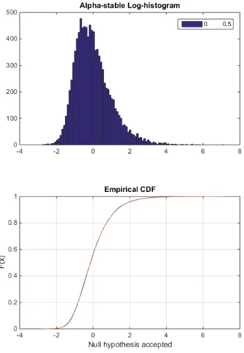
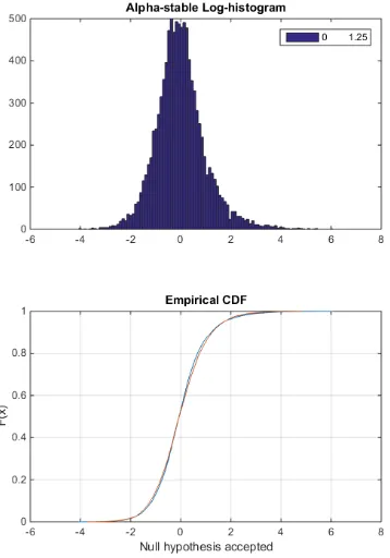
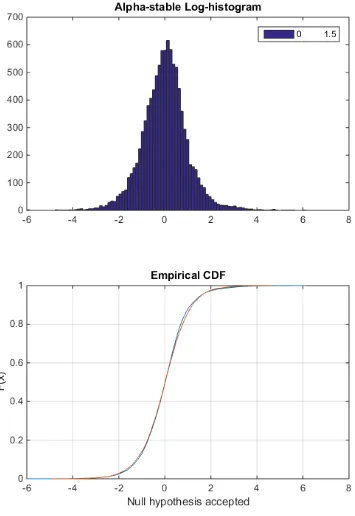
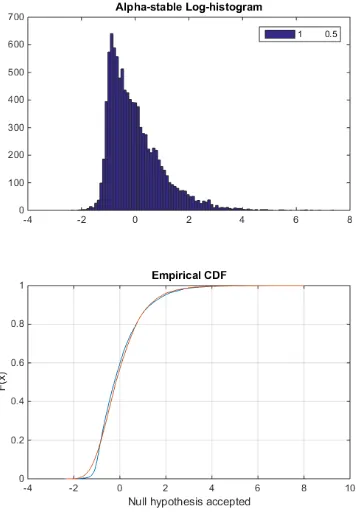
With parameters (α, d, g) , generate HGO distributed data Z1 and finally perform a Two sample Kolmogorov-Smirnov test.

(61)

Chapter 4. Log-compressed data modeling 45

H = 0 => Do not reject the null hypothesis at the 5% significance level.

H = 1 => Reject the null hypothesis at the 5% significance level.

Let S1(z) and S2(z1) be the empirical distribution functions from the sample vectors Z and Z1, respectively, and F1(x) and F2(x) be the corresponding true (but unknown) population CDFs. The two-sample K-S test tests the null hypothesis that F1(z) = F2(z1) for all z, against the alternative that they are unequal.

The decision to reject the null hypothesis occurs when the significance level equals or exceeds the P-value= 0.05.

4.6 Concluding Remarks

(62)

46 Chapter 4. Log-compressed data modeling

FIGURE 4.1: Montecarlo experiment for testing the HG0 distribution

Electromagnetic models for ultrasound image processing

P

H

D T

HESIS

Electromagnetic Models for Ultrasound

Image Processing

Declaration of Authorship

Acknowledgements

Contents

List of Figures

Dedicated to My Parents María Elvia (in memoriam) and Jesús

Francisco. To My Sisters and Brothers: José "Froidon" (in

memoriam), Carlos Alberto "Lagüete", Carmenza "Mana",

Marcelo "March", Aristóbulo "Lacrija", Marina "Palela",

Clementina "Tina" (in memoriam), Solón "Ranitas", Jairo

"Yaripal", Sandra "Lachanda" and Elkin "Burropín". To My Wife

Mónica. And to my son, Hugo Alberto

Abstract

Prologue

Motivation

Objectives

Contributions

Thesis outline

Chapter 1

Introduction

1.1

General Considerations

1.2

Central Limit Theorem Approach

1.3

Compound Representation Approach

1.4

Multiplicative Model Approach

1.5

Logarithmic compression

Chapter 2

Statistical Models for Ultrasound RF

data

2.1

Central Limit Theorem Approach

2.2

Compound representation approach

2.3

Multiplicative model approach

Chapter 3

A general model for ultrasound

B-scan images

3.1

Statistical models for SAR data

3.2

G

3.3

G0 distribution for ultrasound image processing

3.4

HG0 distribution for Log-compressed B-scan images

3.5

Moments generating function method for HG0 parameter

estimation

R

3.6

Maximum likelihood method for HG0 parameter

estima-tion

Chapter 4

Log-compressed data modeling

4.1

Montecarlo simulation of Log-compressed data

4.2

Homodyned-K distributed data simulation

4.3

Stable process simulation

4.4

Log Compression

4.5

HG0 distribution for modeling Log-compressed data

4.6

Concluding Remarks