Unemployment duration, unemployment benefits and recalls

Texto completo

(1)Working Paper 06-62 Business Economics Series 18 October 2006. Sección de Organización de Empresas de Getafe Universidad Carlos III de Madrid Calle Madrid, 126 28903 Getafe (Spain) Fax (34) 91 624 5707. UNEMPLOYMENT DURATION, UNEMPLOYMENT BENEFITS AND RECALLS* Alfonso Alba-Ramírez1, José María Arranz Muñoz2 and Fernando Muñoz-Bullón3. Abstract We use administrative micro-data to investigate exits from unemployment of benefit recipients in Spain. Because the data allow us to distinguish between transitions to a new job and recall to the same employer, we apply a competing risks model with observed and unobserved heterogeneity. We are also able to control for the type of benefit received by the worker: insurance benefit or assistance benefit. We find significant differences between the new job hazard and the recall hazard. Both hazard rates increase around the time that insurance benefit elapses. We also find that when larger firms recall unemployed workers they tend to do so faster than smaller firms. In general, our results are consistent with predictions derived from search and implicit contract models. They highlight the importance of taking into account the possibility of recall in the analysis of unemployment duration among unemployment benefit recipients.. Keywords: unemployment duration, recall hazard, new-job hazard, unobserved heterogeneity, unemployment benefits, competing risks model. Codes: C41, J64 1. Universidad Carlos III de Madrid. Departamento de Economía. C/Madrid, 126. 28903 Getafe (Madrid). SPAIN 2 Universidad de Alcalá, Departamento de Estadística, Estructura y OEI, Plaza de la Victoria 3, 28803 Alcalá de Henares (Madrid). SPAIN. 3 Universidad Carlos III, Sección de Organización de Empresas, C/Madrid 126-Getafe (Madrid), 28903 (Spain); fernando.munoz@ uc3m.es * We would like to thank seminar participants at the European Association of Labour Economics conference 2006 (Praga) for helpful suggestions. We are very grateful to the Spanish Ministry of Labour and Social Affairs for financial support and the data used. Financial support was also provided by the Ministry of Education and Science, project SEC2003-08714. Only the authors are responsible for any errors.. 1.

(2) 1. Introduction Workers in temporary layoff are those whose unemployment spells end in reemployment by the previous employer. Previous literature has paid attention to the fact that individual transitions out of unemployment depend on the extent to which recall by the previous employer is expected (Katz, 1986; Jensen and Westergård-Nielsen, 1990; Corak, 1996; Rosholm and Svarer, 2001; Jensen and Svarer, 2003; Røed and Nordberg, 2003). This literature has also found significant differences between the effects of the explanatory variables on the recall and the new job hazard rates. In particular, firm incentives (the degree of experience rating) play a key role in the timing of recalls, in so far as the publicly financed temporary dismissal period (with unemployment benefits) may be a direct subsidy to firm-specific pools of labour (Feldstein, 1975, 1976; Baily, 1977). Given that the Spanish unemployment compensation system (UCS) does not contain any element of “experience rating” for contributions, the system may offer an implicit subsidy to firms that make more use of temporary layoff. In this setting, when the need for a temporary employment adjustment arises, Spanish firms may be relying more on temporary layoffs —and less on other adjustment mechanisms— because they can shift part of the cost of the adjustment to the public purse through the UCS. Indeed, recent studies of unemployment duration in Spain —see Alba et al. (2007)— have shown that a large proportion (roughly, 37 per cent) of all unemployment spells in Spain end in recalls. Although this figure is lower than those reported for the US and Canada1, it is comparable to what has been estimated for other European countries: In Denmark, around 50 per cent of all unemployment spells are due to temporary layoffs (Jensen and Svarer, 2003); in Sweden about 45 per cent of all transitions from unemployment end in recalls to the previous employer (Jansson, 2002); in Germany the recall rate has been estimated at 26 per cent (Mavroramas and Orme, 2004); in Austria 32 per cent of all unemployment spells ended with the individual returning to the previous employer (Fischer and Pichelmann, 1991). The aim of this paper is to investigate unemployment duration determinants of benefit recipients, distinguishing between unemployment insurance and unemployment assistance benefits. We use a sample of newly unemployed workers, that is, workers who entered unemployment in the first semester of 2000. We take into account that worker can become re-employed with the previous employer or with a new employer. The former type of re-employment corresponds to the unemployment being a temporary layoff (i.e., a recall). For these purposes, we apply a competing risks model to the duration of unemployment accounting for observed and unobserved heterogeneity. This model allows for two routes for leaving unemployment —a new job or recall— and provides specific estimates of the effects of covariates on each exit hazard. The interest of this analysis is threefold. First, recalls may be viewed as the result of implicit re-employment contracts, so that some individuals may be subject to working for the minimum amount of time needed to qualify for UI benefits (1 year), collecting them for as long as possible (up to 4 months), being recalled to the previous employer, 1. Larger recall rates in the US and Canada economies are well documented. In Spain, a highly regulated labour market imposes many constraints on the hiring and firing decisions of firms. For instance, Robertson (1989) reports that more than 50 per cent of total unemployment spells in Canada are terminated because the worker returns to the previous employer; Katz and Meyer (1990) report that 57 per cent of all unemployment spells in Missouri and Pennsylvania (USA) are temporary layoffs.. 2.

(3) and, then, repeating the cycle. If this were the case, we would expect the hazard rate to rise as the moment of unemployment benefit exhaustion approaches2. Second, very few works research the forces behind the duration pattern of recall for unemployment benefit recipients (see for instance, Katz and Meyer, 1990; Corak, 1996; Mavromaras and Rudolph, 1998; Røed and Nordberg, 2003 and Mavromaras and Orme, 2004), in spite of large evidence on the effect of unemployment benefits on the unemployment hazard rate3. Third, we focus on differences in recall patterns among benefit recipients with unemployment insurance benefits versus those under unemployment assistance benefits; this constitutes a novelty, as the Spanish literature has only offered evidence on the effect that the amount and entitlement duration of each benefit system has on the unemployment hazard rate without disentangling the type of exit: new job or recall (see Cebrián et al.,1996; Alba-Ramírez, 1999; Bover et al., 2002; Jenkins and GarcíaSerrano, 2004; Arranz and Muro 2004 and 20074. Our results show that not only do individual characteristics influence recall and new-job hazard rates differently, but also that their duration dependence patterns also differ. Second, while the probability of leaving unemployment through recall or a new job increases greatly around the time of UI exhaustion, the recall hazard rate of UA recipients decreases when benefit runs out and increases thereafter. These results suggest that the duration of benefits may have a strong influence on firm recall policies and workers’ new job finding behaviour. Finally, we see that larger firms (especially in the industry sector) tend to recall their workers faster than smaller firms. The paper is organised as follows. Section 2 gives a brief description of the Spanish UCS. Section 3 describes the data and variables. Section 4 presents the competing risk duration model. Section 5 disentangles estimation results for unemployment insurance and unemployment assistance benefits recipients. Finally, conclusions are given in section 6.. 2. This is a well known finding (Ham and Rea, 1987; Katz and Meyer, 1990; Hunt, 1995; and Carling et al.,1996). Other studies like Fallick (1991) and Narendranathan and Stewart (1993) find that the effect of UI decreases over time, and Micklewright and Nagy (1998) did not find any rise in the hazard near the time of benefit exhaustion. 3 While some studies have found no effects of the unemployment insurance (UI) level on unemployment duration (Lynch, 1989; Hujer and Schneider, 1989; Groot, 1990), there are many studies that report a negative and significant effect (Narendranathan et al.,1985; Van den Berg, 1990; Katz and Meyer, 1990). Other work has found that the UI level increases job search intensity (Blau and Robins,1990; Wadsworth,1990). Regarding the effect of unemployment assistance benefits (UA) on exits from unemployment studies are scarce. Micklewright and Nagy (1999) find that the UA level discourages the unemployed search effort; Earle and Pauna (1998) detect that the effect is null; finally, Erbenova et al. (1998) and Earle and Pauna (1998) find a work disincentive effect of UA entitlement duration on the unemployment hazard rate. 4 Most Spanish works do not contain information on the level and entitlement duration effect (e.g., AlbaRamirez, 1999; Bover et al., 2002). The ones that take this information into account find either that UI levels do not exert a clear negative influence on unemployed job search behaviour (Cebrián et al.,1996), that UI levels increase the unemployment hazard rates temporarily and that the UA level reduces the job search intensity (Arranz and Muro, 2004 and 2007), or that the hazard rate of UI recipients rises dramatically when UI benefits exhaustion approaches (Jenkins and García-Serrano, 2004, and Arranz and Muro, 2004 and 2007).. 3.

(4) 2. The unemployment compensation system in Spain In this section we describe the Spanish UCS as it stood in 2000, which is the starting point for the data set on unemployment duration used in this article5. As in other European countries, the Spanish UCS is composed of two parts: unemployment insurance (UI) and unemployment assistance (UA). The UCS is financed with a payroll tax of about 7 percent, of which approximately 80 percent is charged on the employer and 20 percent on the employee; and it is not experienced rated. Eligible for UI are workers whose unemployment situation is recognized according to law by the labour authority; i.e., the job was lost involuntarily, including end of a fixedterm contract. Eligibility requires Social Security contributions for a minimum of twelve months during the six years preceding unemployment. Workers who made contributions for 12-17 months are eligible for 4 months; a contribution of 18-23 months entails 6 months, and so on to a maximum of 24 months of UI for those who contributed to Social Security for 72 months or longer (see Table 1). The amount of UI is determined as a percentage of the average wage in the twelve months preceding unemployment. It is 70 percent during the first six months of unemployment, and 60 percent the remaining period of eligibility. The minimum amount of UI is 75 percent of the statutory minimum wage (SMW) if the worker has no dependent children and 100 percent if he or she has dependent children. There is also a maximum equal to 170 percent of the SMW, which is raised to 190 percent if the unemployed person has a dependent child, and 220 percent if he or she has two or more dependent children. [TABLE 1] UA is financed through transfers from the public budget and it is granted to unemployed persons whose total income does not exceed the minimum wage and are in one of the following situations: (1) exhausted UI and have family dependents; (2) aged 45 years or older and received UI for at least 12 months; (3) did not meet the minimum contribution period for eligibility; (4) returned from foreign migration; (5) was released from prison; (6) an invalidity spell ended by the labour authority declaring the worker able to take a job; (7) aged 52 or older6. The amount of UA has no relation with the previous monthly wages. A family income criterion is also used whereby per capita family income could not exceed the SMW. A flat rate equal to 75 percent of the SMW is paid to all beneficiaries, except for workers aged 45 or older who received UI for 24 months. Their benefits vary with the number of family dependents: 75 percent of the SMW if one or no family dependents, 100 percent if two family dependents and 125 percent if three or more family dependents. UA is time limited and it is conditioned on which of the above indicated situations the worker is, of being 45 or older, and on having or not family dependents (see Table 1).. 5. The Spanish UCS was reformed in 1992 in order to increase entitlement requirements and to reduce benefit amounts. A previous change took place in 1984, and a minor change on the UA in 1989. 6 Also, special UA is available to workers of the agricultural sector who have residence in the autonomous communities of Andalucia and Extremadura.. 4.

(5) 3. Data, variable definitions and descriptive analysis 3.1. The data This paper uses a sample of individuals who entered unemployment in the first semester of 2000 and started receiving unemployment benefits. The data have been extracted from the HSIPRE (Histórico del Sistema Integrado de Prestaciones), a Spanish administrative data set that provides information on unemployment benefits received by each worker. The dataset includes information on the type of benefits received (UI or UA), the number of days granted for benefits, the number of days of benefit receipt, the number of children the individual has, the benefit level, and previous earnings for each individual. The quality of this data set is deemed to be high (see Jenkins et al., 2004; Arranz and Muro, 2004 and 2007). In order to enrich the possibilities of our empirical analysis, we have merged the described data with a data extracted from Spanish Social Security records. The latter contain information on all employment (and non-employment) spells of workers in the Spanish labour market over a three-year period (from June 1999 to June 2002). This way, we dispose of information on benefit recipients belonging to the HSIPRE dataset regarding their age, gender, qualification level7, dates of start and end of employment spells, reason for termination of each spell (voluntary/involuntary or retirement), province of residence of the worker, an identifier of whether employment spells are accomplished through a temporary help agency (THA) or not, the type of contract held by the worker (temporary or permanent), and firm size. The advantage of using Social Security data for the analysis of flows in and out of nonemployment is threefold8: (i) We have information on all jobs held by the individual during a certain interval of time; (ii) non-employment duration is very accurate and detailed; (iii) it is possible to distinguish spells ending through recall from those ending through the finding of a new job. In addition, the combination with data from the unemployment benefits receipt allows us to overcome many of the limitations of studies that use data from either Social Security records or the HSIPRE. In some instances, Spanish studies using only Social Security data —e.g., García-Pérez and Muñoz-Bullón (2005a)— are unable to distinguish whether or not the individual is receiving unemployment benefits. Studies using data sets such as the Integrated Benefits System have information on level and unemployment benefit duration (current and entitlement) of recipients (Arranz and Muro, 2004 and 2007; Cebrián et al., 1996; Jenkins et al., 2004). Nevertheless, none of these works distinguishes spells ending through recall from those ending through the finding of a new job.. 7. The qualification level indicates a position in a ranking determined by the worker's contribution to the Social Security system. Therefore, although it is somewhat related to the individual's qualification level — since it reflects the worker's professional category and salary— it does not reveal the workers' level of qualification, but rather the required level of qualification for the job. It may be the case, however, that a worker with higher education is far below the category that would correspond to his formal education. For instance, an individual working in the lowest category, “labourers”, may well be in possession of an academic degree. As in previous studies using data from the Social Security records, we group those ten categories into four groups (see Table A.1 in the appendix) 8 A different extraction from Social Security records was previously used to study employment and unemployment spells through the use of duration models in García-Fontes and Hopenhayn (1996), García-Pérez (1997), and García-Pérez and Muñoz-Bullón (2005a, 2005b), but they only have data up to the year 1999.. 5.

(6) Since our work focuses on an initial sample of workers who experience unemployment in the first semester of 2000 and start receiving unemployment benefits, we drop individuals who do not meet all the following criteria. 1) Entered unemployment due to involuntary reasons —i.e., dismissals or termination of temporary contracts9. As we consider only the first spell of unemployment occurring in the indicated period, we obtain a “flow sample” of unemployed workers in the terminology of Lancaster (1990), pp. 162; 2) In the previous job, the individual was registered with the General System of Social Security10; 3) The individual starts receiving UI or UA11; 4) We have complete information on all the variables used in the empirical analysis; 5) Workers must remain out of work for more than 30 days. We eliminate workers with unemployment spells lasting 30 days or less because they experiment straight movements from job to job without experiencing unemployment. Finally, we limit our sample to workers aged between 16 and 62 (to avoid complications associated with early retirement). Since each firm is issued an (anonymous) identification number, which is separately recorded for every single spell of employment, recalls can be easily identified. Starting from the unemployment spells under consideration in the year 2000, the characteristics of both its previous and its subsequent spells of employment were determined12. [TABLE 2] After applying the indicated sample selections, we obtain a final sample 6,315 individuals. Descriptive statistics for the explanatory variables used in the empirical analysis are shown in Table 2. We observe that around 29 per cent of all unemployment benefit spells end in recalls. Therefore recalls constitute an important element of unemployment under benefits in Spain. The recall outcome is relatively more present among women (57 per cent of recalled workers are women as compared to 47 per cent in the whole sample), and on individuals with relatively low qualification levels. Moreover, age appears as a relevant determinant of the recall outcome. In particular, workers aged 25-39 are substantially more likely to be recalled. Recalls are also concentrated on individuals enjoying short unemployment duration: workers unemployed between 4 and 20 weeks account for 59 per cent among recalled and 46 per cent among those entering new jobs. Other typical features of recalled workers are that they held a previous temporary contract for a short period of time in a firm with 10 to 50 employees, that they received UI and had no children. On the other hand, the unemployed who enter a new job is more likely to be a male, to be 25 to 29 years old, to have worked in firms with less than 50 employees and to have had longer tenure and unemployment durations. 9. We cannot distinguish between these two reasons for job termination. Workers who quit their jobs (i.e., end their employment for voluntary reasons) are not considered in this study because we do not know why this happens and these workers are likely to leave the labour force (García-Pérez and Muñoz-Bullón, 2005b). 10 Since specific regimes like farming and self-employment have different rules for accessing benefits they are not considered here. 11 We leave for future research the analysis of UA for unemployed have exhausted UI, since UA recipients in our dataset are those who do not meet the minimum contribution period for UI eligibility. 12 We have no information on ex ante temporary layoffs —i.e., those that begin with a person expecting to be recalled. Thus, the ex post measure is likely to underestimate the total amount of unemployment affected by recall prospects, since it does not include the unemployment of those who initially waited for recall but were not recalled. In any case, this ex post concept gives the proportion of unemployment from spells involving no job change (Feldstein, 1975; Clark and Summers, 1979), and it is not ambiguous in the sense that it is not based on whether individuals decided what is a new employer and what is not (see Alba et. al, 2007).. 6.

(7) 3.2. Variable definitions 3.2.1. Benefit-related variables We define a dummy variable that equals 1 at each month the worker receives UA benefits, and zero when UI benefits are received. The impact of unemployment benefits on the hazard is also measured using functions of the time until benefits lapse. We include time until benefit exhaustion dummy variables for seven intervals covering months before and after benefits are expired. These variables are designated “UB>18” through “UB>-10”. Each of these time-varying exhaustion dummies takes on the value of one in its designated interval and takes on the value of cero in all other periods. For example, “UB12-18” takes on the value one when the individual is 12 to 18 months until exhaustion; “UB –5 to –10” takes on the value one when the individual is 5 to 10 months after benefit exhaustion; “UB1, UB0 and UB-1” takes on the value one in the month before benefit exhaustion, the month of benefit exhaustion and the month after benefit exhaustion, respectively. Finally, as a proxy for the compensation variable in a job search model, we compute the replacement ratio as a time varying covariate, which is the relation between the UI or UA benefits level and the previous wage. This variable is expected to be positively correlated with the reservation wage, and, therefore, negatively correlated with the hazard function. Duration-dependent benefit levels for each spell month were calculated by applying the rules of the UI and UA system to the dataset13. Benefit and previous wages were converted to 1992 prices using the monthly retail price index. 3.2.1. Control variables We control for demographic variables such as age at the start of the unemployment spell, using a non-linear specification distinguishing 10 age groups. We also control for gender. Worker’s previous employment history (i.e., job turnover) should be an important explanatory factor of the reemployment probability, since individuals more accustomed to move jobs are supposedly more “employable”, and thus are expected to leave unemployment earlier. Given that the database includes the complete employment history of workers from June 1999, we include as a covariate the number of jobs held previous to the one leading to the spell of unemployment under study. This variable gives us a measure of the number of times they suffered unemployment from that date. In addition, the higher the relative job stability (in terms of tenure) experienced by workers in the previous job, the lower the hazard rate from unemployment into employment will be, due to a higher reservation wage. Tenure in the previous job is included through six dummy variables (<= 1 week, > 1 week and <= 4 weeks, >4 weeks and <=20 weeks, > 20 weeks and <= 1 year, >1 year and <= 2 years, >2 years). The qualification level required for the previous job is collected through four levels of the professional category of the worker contribution to the Social Security. We include a dummy variable indicating whether or not the individual was hired in the previous job 13. A time varying UI level covariate was constructed as a 70 percentage of the average wage (in the twelve months preceding unemployment) during the first six months of unemployment, and 60 percent the remaining period of eligibility. The UA level is a constant (see section 2).. 7.

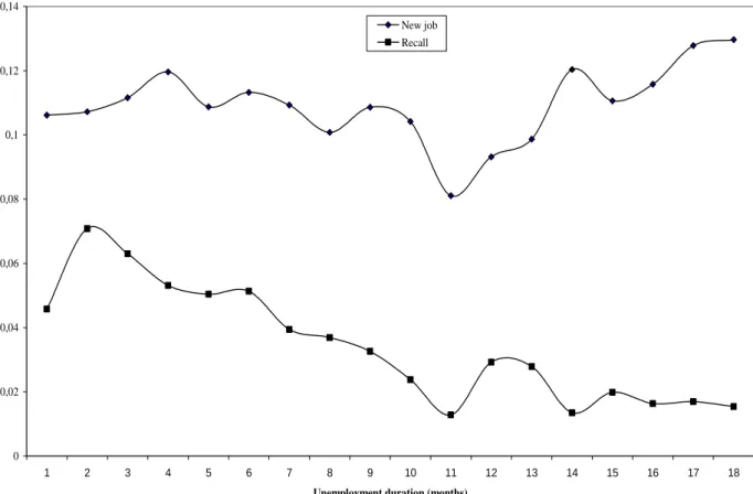
(8) by a temporary help agency (THA). We are able to distinguish whether or not the individual entered into unemployment from a job either with a fixed-term contract, with a permanent contract, or with a permanent per task contract. Workers under this latter type of contract enjoy a strong relationship with their previous employer during the layoff: this relationship is much stronger than with other types of contracts, since individuals retain seniority and other employment-related benefits (for instance, they have the right to return to the same job with the same employer, since they have the privilege of being requested first by their previous employer on their availability to reenter their payroll14). We control for the industry where the worker was engaged at in the previous job: some industries may have more fluctuations in demand or supply than others, which means that the tendency to use temporary layoff as a means of smoothing labour force adjustments is relatively high, other things equal. Regarding firm size, its impact is included through five dummy variables: <=10 workers, >10 and <=50 workers, >50 and <=200 workers, >200 and <=1000 workers and >1000 workers. Regional labour market and household conditions are also taken into account, through dummies for the seventeen Spanish Autonomous Communities and the quarterly regional unemployment rate as a time varying covariate. Seasonal effects are captured by a set of dummy variables indicating whether workers entered into unemployment in January-February, March-April, or May-June. We also include four dummy variables for the number of children: no children, one child, two children and three or more children. Finally, we control for the duration (in months) of the unemployment period by including dummy variables. 3.3 Non-parametric analysis An explanatory data analysis using non-parametric estimation of the hazard rates can provide a first impression of what kind of profile the data exhibit. The following nonparametric analysis is based on life table estimation. The time profiles of the empirical hazards are presented in Figure 1. This figure represents job finding rates for the entire sample making a distinction between recall and new-job. These estimates offer the conditional probability of exiting from unemployment into a new job or recall and how it changes over the course of the unemployment spell. Since there exists a very small number of observations for durations above 18 months and in order to avoid noise in the results, we have considered these observations as artificially right-censored, that is, as unemployment spells that do not finish in the observed period. This is the reason why there are no observations with unemployment durations beyond 18 months. [FIGURE 1] As can be observed in Figure 1, the empirical hazard rate from unemployment into reemployment through recall keeps below the rate from unemployment into a new job finding. On the one hand, the new-job finding rate basically overall presents no duration dependence up to the eleventh month of unemployment. From this month onwards, it increases at an accelerating rate throughout the course of the spell. Spikes at months 4, 6, 8, 12 and 14 can be interpreted from the supply side of the labour market: as the exhaustion of UI benefits approaches, claimants are expected to look harder for a new job, and are more willing to accept a job offer. On the other hand, the recall rate 14. In addition, when being laid-off, those individuals receive payments subsidized by the Government (through the UI system for the time not worked).. 8.

(9) presents positive duration dependence until the second month and negative duration dependence thereafter up to the eleventh month, showing a notable spike around the 12th month of unemployment. However, it finally declines just after the 13th month, remaining close to a flatter line from the 14th month onwards. Thus, on the whole, the longer a worker remains on layoff, the lower his perceived instantaneous recall probability. 4. A competing risks duration model. For the empirical analysis, we specify a discrete-time duration model with competing risks of exits following the formulation proposed by Allison (1982). This same econometric frameworks has been used by Jenkins (1995), Alba-Ramirez (1998), Steiner (2001), Lauer (2003), and D’Addio and Rosholm (2005), among others. This type of models is common in the analysis of temporary layoffs where all the unemployed are subject to the competing risks of a recall and a new job (Katz, 1986; Røed and Nordberg, 2003)15. An advantage of the competing risks model is that we can obtain a neat result for the re-employment probability because we estimate the discretetime hazard model simultaneously for the two kinds of exists from unemployment. In a discrete–time duration model with competing risks, an individual’s unemployment spell is represented by a random variable T, which can take on positive integer values only. We observe a total of n independent individuals (I=1,…,n) beginning at some natural starting point t=1. In the data used in this paper, such point is the month when the worker becomes unemployed for the first time during the first semester of the year 2000. Each observation continues until time t, at which point an event occurs or the observation is censored. The unemployment spell can end, T=t, in any of j states: j=1 (re-employment through a new job) or j=2 (re-employment through the same employer as the immediately previous one; that is, a recall takes place). The observation is censored when the surviving individual is observed at month t but not at month t+1. It is assumed that the time of censoring is independent of the hazard rate for the occurrence of events, at least after controlling for other factors. Also, it is assumed that the set of two states at which unemployment spells end is absorbing and equal for each person. For modelling the transition from unemployment to employment through recall or a different employer, we define the discrete hazard rate. For the i-th person, the hazard rate into state j (j=1,2) in period t, hij(t), is the conditional probability of a transition to state j in this period, given that individual i has been unemployed until t16. hij(t) = Pr[Ti=ti, J=j | Ti>= ti]. [1]. Assuming that the competing risks are independent, the hazard rate from unemployment is given by: 15. A problem when estimating single risk duration models is the potential aggregation bias. Unemployed typically leave unemployment for different reasons (competing risks). Restricting the estimated coefficients for the baseline hazard and the covariates to be the same for all destination states might therefore be a very restrictive assumption. Therefore, the econometric model for the sequence of discrete choice models is a multinomial logit model or competing risks model; in each spell, the unemployed can either stay in unemployment (the reference category), be re-employed though a different employer or be re-employed though the same employer. 16 According to the simple job search model (Lippman and MacCall, 1976), given a stationary reservation wage, the re-employment probability is the result of two probabilities: the rate at which offers arrive times the probability that a random offer is accepted. In our competing risks model, unemployed workers can either obtain a job through a different employer from the immediately previous one or be re-employed through recall to the previous employer.. 9.

(10) 2. hi(t) = ∑ hij(t). [2]. j =1. Assuming that all spell observations are independent, the likelihood function for the original state j can be written in terms of hazard rates as follows:.  2  h (t) δij  t   ij L = ∏∏  ∏(1− hik ) ( 1 h ( t ) −  i=1 j=1   ij   k=1   n. [3]. In this expression, the indicator function δij, equals one if the duration is complete (individual i makes a transition to state j), and equals zero if duration is censored. Therefore, the first component of [3] captures the transition rate and the second component is the survivor function which represents the conditional probability that individual i remains unemployed in period t. Given that [3] is in function of the transition rates, we just need to specify the dependence of the latter on a set of explanatory variables. For the hazard rate we choose the logistic specification that, with multiple events, generates the multinomial logit model (Maddala, 1983). It allows for the three possible states considered: employment through a different employer; employment through recall; and remaining unemployed (which is the reference state category). For individual i, the transition rate to state j in period t specified as a multinomial logit can be written as (Steiner, 2001, pp. 96):. h j ( t | z(t ), ε j ) =. exp(D' (t )α j + Z ' (t ) β 'j + ε j ) 2. 1 + ∑ exp(D' (t )α m + Z ' (t ) β m + ε m ). [4]. m =1. where Z(t) is a vector of explanatory variables which may vary with time; β is the vector of parameters to be estimated; the terms α stands for the baseline hazard which captures the duration dependence. The specification of the baseline hazard is very important. A common but restrictive approach consists of specifying a parametric form for the baseline hazard. This approach is very strong because the assumptions over the form are difficult to justify from an economic point of view, and provokes a misspecification problem. Instead, we choose a semi-parametric approach (piecewise constant hazard) by specifying monthly dummies D(t) which coefficients for transitions to employment through recall can differ from those for transitions to employment through a different employer. This method presents the advantage of being flexible and assumes that the duration dependence pattern may vary among the states. Finally, since failing to control for unobserved heterogeneity in hazard models tends to create spurious negative duration dependence in the baseline hazard out of unemployment (Lancaster, 1979, 1990), in our analysis ε accounts for unobserved heterogeneity characteristics in the model such as motivation, ability, effort, family pressure, etc. We assume that the unobserved heterogeneity effect is destination state specific, time constant, and independent of the observed characteristics17. 17. This is a standard assumption in duration models (D’Addio and Rosholm, 2005; Jenkins, 1995; Rosholm and Svarer, 2001; Steiner, 2001). If this assumption is violated, maximum likelihood estimates will be biased by endogeneity. That is, the estimated β coefficients will pick up some of the effects of the unobservable characteristics, ε. If we relax the assumption and ε is correlated with Z, then the probability of exiting from unemployment through a new job or by recall will be affected, and a test for endogeneity. 10.

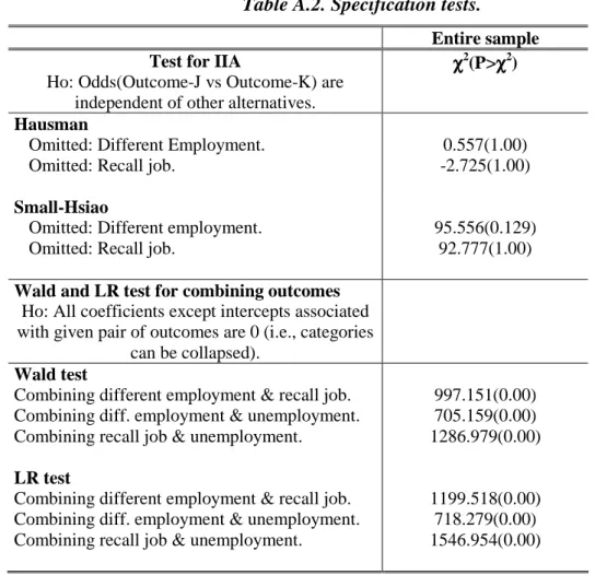
(11) The contribution to the likelihood function for a single individual is equal to (D´Addio and Rosholm, 2005, pp. 454): t. L( β , α | ε ) = ∏. [. exp ( Dk' α 1 + Z k' β 1 + ε 1 ) c1k + ( Dk' α 2 + Z k' β 2 + ε 2 )c 2 k. k =1. 2. 1 + ∑ exp( D α m + Z β m + ε m ) m =1. ' k. ]. [5]. ' k. where cjk are indicators for making the transition to each of the possible destination states at time k; re-employment through a different employer from the immediately previous one (j=1), or re-employment though the same employer as the immediately previous one (j=2). Unemployment spells that are still in progress at the end of the observation period are treated as right censored observations. For these observations, both destination indicators are 0, and thus, the contribution to the likelihood function is the probability of remaining unemployed for at least the observed sample period. In [5] a common procedure is to specify a parametric distribution for the unobserved heterogeneity such as a normal, gamma distribution, etc. However, given that the unobserved heterogeneity distribution is unknown, Heckman and Singer (1984) have criticised this approach, showing that parametric form assumptions for unobserved heterogeneity might be biased when the chosen distribution for the unobservable term is incorrect. For this reason, they resolve this problem by assuming that unobserved heterogeneity is discretely distributed with unknown support points. Those points can be interpreted as latent individual's types. Then, the likelihood function for an individual may be obtained by integrating the following conditional likelihood distribution: S. L( β , α , ε , π ) = ∏ L(β , α | ε = s )π ( s ). [6]. s =1. Where ε are the location points (that can be interpreted as intercept for the baseline hazard function), π the probability associated to them, and s the number of support points18. In the following section we estimate this likelihood function by maximum likelihood to know how individual and labour market characteristics influence unemployment spell durations via recall or a new job19.. 5. Estimation results will be required. As proposed by Heckman and Borjas (1980) and Chamberlain (1985), the identification in such models relies in the specification in terms of leads and lags of all the time varying covariates such that their lagged values can be used as instruments for the variables that may be suspected of endogeneity. This is only practical if there is sufficient variation over time in regressors. However, identification of a model where a test for endogeneity could be implemented results infeasible due to the short span of our sample period (see, in this respect, D’Addio and Rosholm, 2005, pp. 454). 18 It should be indicated that the econometric approach adopted in this article boils down to estimating a reduced form model for employment transitions, conditional on a set of individual and job characteristics and on the worker being in a particular initial state. Other features that make this technique an attractive and flexible one for estimating the effect of those characteristics on the probability of exit from unemployment are: 1) The consideration of competing risks; 2) The incorporation of individual specific unobserved heterogeneity; and 3) The fact that no assumptions are made with respect to the shape of the baseline hazard. 19 We have performed tests for the assumption of ‘independence of irrelevant alternatives’ (IIA) through the Hausman test (Hausman and McFadden, 1984) and Small Hsiao test (Small and Hsiao, 1985) in Table A.2 in the appendix. In both tests, the null hypothesis of IIA is accepted; therefore, the multinomial logit specification seems to be appropriate for each arrival state (new job or recall). In addition, a Wald test and a LR test were performed in order to examine the null hypothesis that the coefficients of each category do not differ significantly from each other, for all the possible combinations. The rejection of the null hypothesis means that it is adequate to distinguish between exits into a new job and a recall job; therefore, the multinomial specification seems to be appropriate, since none of the categories should be combined.. 11.

(12) In this section, we present the empirical results from the estimations of the model outlined in Section 4. Estimations have been obtained based on the likelihood function (6) by the maximum likelihood estimator. First, we present the results from the competing risks model for the entire sample in Table 3 (Table A.3 in the appendix shows the results separately for men and women). Second, we present in Table 4 the results separately for individuals who receive UI and for those who receive UA. Given that both support points are highly significant in all the estimations, exit rates from unemployment to a new job or recall are affected not only by measured individual and job characteristics of the unemployed, but also by their unobserved characteristics. Estimated coefficients and the value of the log-likelihood are affected by the inclusion of unobserved heterogeneity. In particular, unobserved heterogeneity increases the loglikelihood values in the estimations, which indicates an improvement in the fit of the model.20 5.1. Results for the entire sample A number of explanatory variables have effects that are similar across both exit routes from unemployment (Table 3). In general, these effects are in line with our expectations. Individuals with temporary contracts in their previous employment have a higher escape rate from unemployment compared to those with permanent contracts. The size of the replacement ratio has an inverse effect on the escape rate. Individuals subject to higher turnover (in terms of the number of previous jobs held) enjoy a higher escape rate from unemployment, and the hazard rate out of unemployment increases as the moment of benefit exhaustion approaches. Finally, concerning the effects of benefit variables, UI recipients leave unemployment sooner than those receiving UA. In particular, UA recipients are 18 per cent (34 per cent) less likely to exit from unemployment into a new job (recall job) than UI recipients. This result is consistent with the existence of implicit contracts between firms and UI recipients: workers with above-average attachment are recalled faster by the firm that laid them off. This result may be reflecting a “last-out-first-in” effect in so far as firms prefer to first re-hire workers they already know and value (which is typical of UI recipients). [TABLE 3] Regarding cause-specific effects of the explanatory variables on the hazard rates, the most conspicuous effects are found for the variables age at unemployment spell, type of contract, firm size, tenure in previous job, number of children and gender. People who are under 35 years old have a lower cause-specific hazard rate for being recalled to the previous employer. This negative impact on the recall hazard rate is most probably caused by demand side effects in the sense that the employers do not want to rehire persons with insufficient firm-specific human capital (given its high cost of acquisition in the open market). In addition, it is possible that young workers are deliberately 20. A simple likelihood ratio test of a model with unobserved heterogeneity against another without unobserved heterogeneity confirms the conclusion that unobserved heterogeneity is significant. Thus, the specification with unobservables is identified in the standard multilogit model which is implicit in the text. The value of the likelihood ratio test statistic for the entire sample of a model with unobserved heterogeneity against that without is 165.716. This value exceeds the critical chi square value of 5.99 for 2 degrees of freedom at significance level of 5% and therefore, unobserved heterogeneity component should be included in the specification of the model. The values of the likelihood ratio test statistic are 120.514 and 27.416 for UI and UA recipients, respectively. Both values exceed the critical chi square value for 2 d.f. at significance level of 5% previously mentioned. Therefore, unobserved heterogeneity is also significant in those models.. 12.

(13) searching for new jobs that more accurately match their preferences (which may very well be varying for young persons). For the type of contract, the effect of the permanent per task category on the recall hazard rate is positive whereas it is negative (although statistically non-significant) on the new job hazard rate. It is not difficult to find a convincing explanation for this result, since workers with such contracts are treated as if they had maintained their employment relationship. Thus, they usually do not engage in job-seeking activities because they regard themselves as employed and they are virtually certain to return to their jobs at the end of the layoff period. One important variable that provides interesting insights into the way workers exit unemployment in Spain is firm size. Two relevant factors are associated with firm size: the effectiveness of workers’ representatives and the cost of layoffs for the firm. In Spain, firms can have two types of workers’ representatives: the unions (secciones sindicales) and the workers councils (comités de empresa). Given that the latter are internal bodies formed by employees of the firm, their existence and effectiveness depend on firm size. In particular, workers councils can only exist in firms with at least fifty employees, and have gained an increasing prestige among workers since the early 1980s21. In larger firms, therefore, the relevant legislative constraints that determine the size and effectiveness of the workers councils are considerably more restrictive with respect to the optimising behaviour of firms (Mavromaras and Rudolph, 1998). Given the costs borne by workers in recalls —in terms of losses in current income, future benefit entitlements and employment security— councils are expected to effectively minimize layoff durations in larger firms. Moreover, smaller firms can be expected to experience longer recall durations because individual workers employed by smaller firms will be less able to influence the timing of such recall. As firm size increases, there will be more and stronger workers councils with both the power and the incentive to intervene and assist workers’ optimising behaviour. Our results are consistent with these predictions, for we find that the hazard rate of exiting from unemployment through recall increases with firm size. As regards tenure in the previous job, the recall hazard rate is larger for individuals whose previous tenure is under 4 weeks than for the remainder ones, whereas this variable is statistically non-significant for the new job hazard rate. Finally, the number of children reduces the hazard rate for leaving unemployment to a new job, and women are more likely recalled (whereas men are more likely to re-enter into employment with a different employer). 5.2.Separating the effect of UI and UA We now separate UI recipients from UA recipients in the analysis of the determinants of recall and new job hazard rates. The reason for a distinction between UI and UA is twofold. First, they are different unemployment benefits schemes whose characteristics and objectives differ. On the one hand, UI is received by those unemployed workers who have worked for a minimum contribution period (twelve months) and its level is a percentage of the worker’s previous earnings. On the other hand, those who are not entitled to UI might receive UA. Their entitlement duration depends on age, on whether they have family burdens, and the benefit level is based on the National Minimum 21. The available evidence show greater importance of workers councils as workers representatives along time (Jimeno and Toharia, 1993; Malo, 2005).. 13.

(14) Wage (see Section 2 above). In addition, UI allows job seekers to receive offers with more attractive wages, and thus, in theory, to secure more productive jobs, whereas UA is granted to unemployed with low incomes in order to reconcile the objective of social equity. Second, according to estimation results for the entire sample (see previous section), it is reasonable to expect UI to be the benefit payment leading to a faster estimated recall (and a stronger worker-firm attachment), while, by contrast, workers under UA are expected to have weaker attachment to their former employer (and thus, an estimated prolonged recall duration, as was obtained in previous section). Thus, the distinction between UI and UA is pertinent in the comparison between contract and search models (see, for example Mavromaras and Orme, 2004). Most of the control variables in Table 4 have different effects on the two hazard rates. The time profiles of the recall and new job hazard rates differ by gender, age, qualification level, tenure in previous job, number of children, firm size, activity sector, labour demand (regional) conditions, and by whether or not the individual has worked through a temporary help agency. Men have a larger cause-specific hazard for exiting from unemployment through a new job (under both type benefits). However, they are less likely to be re-employed by the previous employer when UI are being received. Age is an important determinant of recall hazards for both types of unemployment benefits recipients. The youngest unemployed (below 30 years old) have the lowest transition rates from unemployment to a recall job than their older counterparts. The interpretation of this estimated effect is similar to the one obtained for the entire sample (demand side effects). UI recipients with the highest and the lowest qualification levels are more likely to exit from unemployment through recall, while the qualification level presents a nonsignificant impact on the recall hazard rate for UA recipients. Results regarding tenure in the previous job are similar to those obtained for the entire sample: the recall hazard rate is larger for individuals whose previous tenure is under 4 weeks than for the remainder ones. Having worked via a temporary help agency presents a non-significant impact on the hazard rate of exiting from unemployment, with the only exception of UA recipients, whose chances of finding a new job increase up to 80 per cent. There exists evidence of a negative effect of the number of children on the new-job hazard for both types of recipients and a null effect for recall jobs. As regards the state of labour market demand, unemployed who receive UI and live in regions with a lower regional unemployment rate enjoy a higher probability of finding a recall job, since there may be less competition for existing vacancies in their respective locations. As expected, recall durations are shorter for large firms, longer for small firms, and duration of new job spells are not particularly affected by firm size (a similar result is found by Mavromaras et al., 1998). As regards the activity sector, UI recipients from the service sector suffer a lower transition rate from unemployment into a recall job than those from the industry sector. This result is expected in so much as workers from the industry sector (particularly larger firms) move from one job to another with a relatively high frequency. We also appreciate that workers receiving UI from the service sector are more likely to find a new job. Finally, estimated results regarding the type of contract held in the previous job show that duration of recall spells is shorter for benefit recipients who have held either a temporary contract or a permanent per task contract in the previous job (independently of whether they receive UI or UA). This is reasonable, to the extent that, as commented in the previous section, workers under this latter type of contract enjoy a stronger relationship with their previous employer while they are unemployed. [TABLE 4] 14.

(15) Interesting insights arise from unemployment benefit-related variables (time until exhaustion and replacement ratio). The effect of entitlement duration on the probability of leaving unemployment is significantly different according to the route taken back to work. Unemployed receiving UI benefits enjoy an increase in their transitions into new jobs as the moment of benefit exhaustion approaches; a decline in this hazard is observed after benefit exhaustion. This behaviour reflects the joint effect of a falling reservation wage and rising job search intensity in transitions into a new job — Mortensen (1977). As for UI recipients who exit unemployment through recall, there exists an increase in the recall hazard rate around the time of benefits exhaustion, and a null effect is observed thereafter. This result is similar to the one arising from an implicit contract type explanation as described by Feldstein (1976): firms may be extensively using the UI system in downturns to the firm’s demand through a rotating system of layoffs in which workers who exhaust their UI benefits are being recalled, and other workers still eligible for benefits laid-off in their place. Thus, firms expecting recall within a reasonable horizon recall workers close to when benefits run out rather than potentially losing them to new jobs. In contrast, the hazard rate for UA benefit recipients into a recall job decreases when UA exhaustions approach (and only increases after some time has passed from the exhaustion of benefits). Remember that those workers are expected to be less likely to have formed an implicit contract with their previous employer: thus, the recall of UA recipients will take longer and might well happen after UI recipients have become re-employed. The effect of the replacement ratio on both cause-specific hazard rates presents a ∪ form for UI recipients. For UA recipients, the replacement ratio exerts a strong negative impact on both types of exists from unemployment, and this negative effect is lower for individuals who are recalled. [FIGURE 2] Finally, let us first consider estimated duration dependence for UI recipients. Figure 2 shows the estimated hazard rate (after controlling for observed and unobserved heterogeneity) at mean of covariates for UI recipients. As can be observed, new job hazard rates are above estimated recall hazard rates. This result is sensible to the extent that recalls may carry a higher wage due to the accumulation of firm-specific human capital.22 In addition, as regards the new job hazard rate, there exists no duration dependence up to the eleventh month, but there exists positive duration dependence thereafter. As regards the recall hazard rate, there exists positive duration dependence up to the second month and negative duration dependence thereafter. Hence, both hazard rates show different duration dependence patterns, and these results clearly illustrate the danger of estimating a single risk hazard rate, instead of a competing risks model. Our interpretation of these results is that revised expectations of the recall probability result in increased search activity as unemployment duration lengthens, which increases the new job hazard rate. Moreover, since the risk of losing employees on temporary lay-off increases with unemployment duration, this would tend to yield earlier recall by the employer. These results are coherent with the ones found by Katz (1986), Katz and Meyer (1990), Corak (1996), and Jensen and Nielsen (1999).. 22. Fallick and Ryu (1997) present a theoretical model consistent with the indicated relationship between the recall and the new job hazard.. 15.

(16) Moreover, we notice that there are spikes in the rates at which firms recall their temporary-dismissed workers in the period just prior to the exhaustion of UI benefits23.. 6. Conclusions In this paper we have analysed transitions out of unemployment for benefit recipients in Spain considering two alternative ways of becoming employed: recall by the previous employer or reemployment in a new job. The data set used in our analysis contains information on all employment and unemployment benefit spells of workers in the Spanish labour market over a three-year period (from June 1999 to June 2002). They have been generated by combining unemployment benefit records produced by the Spanish Employment Office with Social Security data. Using this rich data set, we have estimated a discrete-time duration model with competing risks of exits to a recall or new job. Duration dependence is accounted for by using a semi-parametric piecewise constant hazard estimation. Unobserved heterogeneity is also taken into account. We have taken advantage of a rich data set that contain information on characteristics of workers and jobs, on duration of unemployment and on unemployment benefit related variables. Among the latter, we have been able to distinguish between the two unemployment benefit systems: unemployment insurance and unemployment assistance. In Spain, unemployment insurance is a function of previous earnings and eligibility requires Social Security contributions for a minimum of twelve months during the six years preceding unemployment. Unemployment assistance has no relation with previous earnings and eligibility is achieved when the unemployed do not meet the minimum contribution period for UI eligibility but have, at least, contributed for 3 months. The competing risks model has turned out to be a good empirical framework to investigate the relationship between exits from unemployment and the receipt of benefits. It has allowed us to find several important differences between the effects on the two cause-specific hazard rates in relation to the type of benefits. The time profiles of the recall and new job hazard rates differ by gender, age, qualification level, firm size, activity sector, by whether or not the individual has worked through a temporary help agency and by labour demand conditions. The hazard of being recalled to the same employer is reduced for recipients below 30 years old. In contrast, the recall job hazard rate is higher for qualified UI recipients who live in regions with lower regional unemployment rate, and, also, for women, for individuals who work in relatively large firms, and for those belonging to the industry sector. In addition, we have found that duration of recall spells are shorter for UI and UA recipients who have held either a temporary contract or a permanent per task contract in the previous job. Comparing benefit schemes, UI recipients leave unemployment sooner than UA recipients. Given that UI is typically received by workers with high worker-firm attachment, this result offers support for implicit contract-type explanations. On the contrary, UA is typically received by workers with low worker-firm attachment. We 23. As regards UA benefit recipients, the estimated recall hazard rate keeps above the hazard rate for unemployed who receive UA and find a new job (figure not shown, but available from the authors upon request). Moreover, the recall hazard rate steadily exhibits positive duration dependence during the first months (up to the eighth one) and negative duration dependence thereafter, while the predicted hazard for new jobs presents no duration dependence across time. We are able to observe that there are some spikes after the exhaustion of UA entitlement durations because our data contain employment transitions before and after benefit exhaustion.. 16.

(17) find a negative recall effect for UA recipients, a result that offers support for job search explanations (Mavromaras and Orme, 2004). Our results show that one of the most important determinants of the probability of exiting from unemployment is the exhaustion of benefits because the hazard rate for UI recipients is higher around that time. Why should the recall rate display a spike as benefit exhaustion approaches when the recall decision is at the discretion of the firm? Two potential explanations are due. On the one hand, some UI claimants appear to search more intensively for a new job as benefit exhaustion looms or become more willing to accept any job offer. However, before doing so, they may attempt to secure recall from their previous employer. On the other hand, UI receipt helps firms to keep a pool of laid-off workers that can be recalled because they are less pressured to find work. The recall of UI recipients could be timed with duration of benefits. We have also provided evidence that the recall of UA recipients is mainly observed after the exhaustion of benefits has taken place. This could be interpreted in a context of firms being more interested in recalling UI recipients because of their higher job attachment. Firms recall UA recipients only after UI recipients are already recalled or reemployed elsewhere.. 17.

(18) REFERENCES Allison, P.A. (1982). “Discrete-Time Methods for the Analysis of Event Histories”, in Leinhardt, S. (ed.), Sociological Methodology. San Francisco: Jossey-Bass Publishers, pp. 61-98. Alba-Ramirez, A. (1998). “Re-employment Probabilities of Young Workers in Spain" Investigaciones Económicas, vol. 22, no 2, pp. 201-24. Alba-Ramírez, A. (1999). "Explaining the Transitions Out of Unemployment in Spain: The Effect of Unemployment Insurance", Applied Economics, 31, pp. 183-193. Alba-Ramírez, A., Arranz-Muñoz, J.Mª and F. Muñoz-Bullón (2007). “Exits from Unemployment: Recall or New Job”, Labour Economics (forthcoming). Arranz, J.Mª and Muro, J. (2004). "An Extra Time Duration Model with Application to Unemployment Duration Under Benefits in Spain", Hacienda Pública Española/Revista de Economía Pública, 171-4, pp. 133-156. Arranz, J.Mª and Muro, J. (2007). "Duration Data Models, Unemployment Benefits and Bias", Applied Economics Letters (forthcoming). Baily, M. N. (1977). “On the Theory of Layoffs and Unemployment”, Econometrica, vol. 45, pp. 1043-1063. Blau, D.M. and Robins, P.K. (1990). "Job Search Outcomes for the Employed and Unemployed", Journal of Political Economy, 98, pp. 637-655. Bover, O., Arellano, M. and Bentolila, S. (2002). "Unemployment Duration, Benefit Duration, and the Business Cycle", Economic Journal, 112, pp. 1-43. Carling, K., Edin, P.A., Harkman, A. and Holmund, B. (1996). "Unemployment Duration, Unemployment Benefits, and Labour Market Programs in Sweden", Journal of Public Economics, 59, pp. 313-334. Cebrián, I., Garcia, C., Muro, J., Toharia, J. and Villagomez, E. (1996). "The Influence of Unemployment Benefits on Unemployment Duration: Evidence from Spain", Labour, 10, pp. 239-267. Chamberlain, G. (1985). “Panel Data”, in S. Griliches and M. Intriligator, eds., Handbook of Econometrics, North-Holland, Amsterdam, 1247-1318. Clark, K.B. and Summers, L.H. (1979). "Labor Market Dynamics and Unemployment: A Reconsideration". Brookings Pap. Econ. Act, 1, pp. 13-60. Corak, M. (1996). “Unemployment Insurance, Temporary Layoffs and Recall Expectations”, Canadian Economic Observer, Statistics Canada, no. 11, May, pp. 3.1-3.15. D' Addio, A.C. and Rosholm, M. (2005). "Exits from Temporary Jobs in Europe: A Competing Risks Analysis, Labour Economics, 12, pp. 449-468. Earle, J.S. and Pauna, C. (1998). "Long-term Unemployment, Social Assistance and Labour Market Policies in Romania", Empirical Economics, 23, pp. 203-235.. 18.

(19) Erbenova, M., Sorm, V. and Terrel, K. (1998). "Work Incentive and Other Effects of Social Assistance and Unemployment Benefit Policy in the Czech Republic", Empirical Economics, 23, pp. 87-120. Fallick, B.C. (1991). "Unemployment Insurance and the Rate of Re-employment of Displaced Workers", Review of Economics and Statistics, 73, pp. 228-235. Fallick, B.F. and Ryu, K. (1997). “Structural Duration Analysis of Lay-off Unemployment Spell: Recall vs. New Job. Draft. Feldstein, M. S. (1975). “The Importance of Temporary Layoffs: An Empirical Analysis,” Brookings Papers on Economic Activity, 3, pp. 725-44. Feldstein, M. S. (1976). “Temporary Layoffs in the Theory of Unemployment”, Journal of Political Economy, 84, pp. 937-57. Fischer, G. and Pichelmann, K. (1991). “Temporary Layoff Unemployment in Austria: Empirical Evidence from Administrative Data”, Applied Economics, 23, pp. 1447-1452. García-Fontes, W. and Hopenhayn, H. (1996). “Flexibilización y Volatilidad del Empleo”, Moneda y Crédito, 202, pp. 205-227. García-Pérez, J.I. (1997). “Las Tasas de Salida del Empleo y el Desempleo en España (19781993), Investigaciones Económicas, vol. 21, pp. 29-53. García-Pérez, J.I. and Muñoz-Bullón, F. (2005a). “Are Temporary Help Agencies Changing Mobility Patterns in the Spanish Labour Market?”, Spanish Economic Review 7 (1), pp. 43-65. García-Pérez, J.I. and Muñoz-Bullón, F. (2005b). “Temporary Help Agencies and Occupational Mobility”, Oxford Bulletin of Economics and Statistics, 67, pp. 163-180.. Groot, W. (1990)."The Effects of Benefits and Duration Dependence on Re-employment Probabilities", Economics Letters, 32, pp. 371-376. Ham, J. and Rea, S. (1987). "Unemployment Insurance and Male Unemployment Duration in Canada", Journal of Labor Economics, 5, pp. 325-353. Hausman, J.A. and McFadden, D. (1984). “Specification Tests for the Multinomial Logit Model”, Econometrica, 52 (2), pp. 1219-1240. Heckman, J.J. and Borjas, G. (1980). “Does Unemployment Cause Future Unemployment? Definitions, Questions and Answers from a Continuous Time Model for Heterogeneity and State Dependence”, Economica, 47, pp. 247-283. Heckman, J.J. and Singer, B. (1984). "A Method for Minimising the Impact of Distributional Assumptions in Econometric Models for Duration Data", Econometrica, 52, pp. 272-320. Hujer, R. and Schneider, H. (1989). "The Analysis of Labour Market Mobility Using Panel Data", European Economic Review, 33, pp. 530-536. Hunt, J. (1995). “The Effect of Unemployment Compensation on Unemployment Duration in Germany”, Journal of Labor Economics, 13 (1), pp. 88-120.. 19.

(20) Jansson, F. (2002). “Rehires and Unemployment Duration in the Swedish Labour Market – New Evidence of Temporary Layoffs. Labour, 16 (2), pp.311-345. Jenkins, S. (1995). “Easy Estimation Methods for Discrete Time Duration Models”. Oxford Bulletin of Economics and Statistics, 57(1 ), pp. 120-138. Jenkins, S.P. and García-Serrano, C. (2004). “The Relationship Between Unemployment Benefits and Re-employment Probabilities: Evidence from Spain”, Oxford Bulletin of Economics and Statistics, 66, 2, pp. 239-260. Jensen, P. and Nielsen, M.S. (1999). "Short- and Long-Term Unemployment: How Do Temporary Layoffs Affect this Distinction?, Working Paper 99-06, Centre for Labour Market and Social Research, Aarhus. Jensen P. and Westergärd-Nielsen N. (1990). “Temporary Layoffs”, in J. Hartog (ed.), Panel Data and Labor Market Studies, North-Holland, Amsterdam. Jensen, P. and Svarer, M. (2003). “Short- and Long-Term Unemployment: How do Temporary Layoffs Affect this Distinction?”, Empirical Economics, 28(1), pp. 23-44. Jimeno, J.F. and Toharia, L. (1993). “Spanish Labour Markets: Institutions and Outcomes”, in J. Hartog and J. Theeuwes (eds.), Labour Market Contracts and Institutions, Elsevier Science Publishers, pp. 299-322. Katz, L.F. (1986). “Layoffs, Recall and the Duration of Unemployment”, NBER Working Paper no. 1825, January. Katz, L. F. and Meyer, B.D. (1990). “The Impact of the Potential Duration of Unemployment Benefits on the Duration of Unemployment”, Journal of Public Economics, 41, pp. 45-72. Lancaster, T. (1979). “Econometric Methods for the Analysis of Duration Data”. Econometrica, 47, pp. 939-956. Lancaster, T. (1990). The Econometric Analysis of Transition Data, Cambridge: Cambridge University Press. Lauer, C. (2003). "Education and Unemployment: A French-German Comparison", Discussion Paper 03-34, ZEW. Lippman, S.A. and J.J. MacCall (1976). “The Economics of Job Search: A Survey”, Economic Inquiry 14, pp. 155-367. Lynch, L. (1989). "The Youth Labour Market in the Eighties: Determinants of Re-employment Probabilities for Young Men and Women", Review of Economics and Statistics, 71, pp. 37-45. Maddala, G.S. (1983). Limited Dependent and Qualitative Variables in Econometrics, Cambridge University Press, Cambridge. Malo, M.A. (2005). “A Political Economy Model of Workers’ Representation: The Case of Union Elections in Spain”, European Journal of Law and Economics, 19, pp. 115-134. Mavromaras, K. G. and Rudolph, H. (1998). “Temporary Separations and Firm Size in the German Labour Market”, Oxford Bulletin of Economics and Statistics, 60 (2), pp. 215226.. 20.

(21) Mavromaras, K.G. and Orme, C.D. (2004). “Temporary Layoffs and Split Population Models”, Journal of Applied Econometrics, 19, pp. 49-67. Meyer, B.D. (1990). “Unemployment Insurance and Unemployment Spells”, Econometrica, 58 (4), pp. 757-782. Micklewright, J. and Nagy, G. (1998). "Unemployment Assistance in Hungary", Empirical Economics, 23, pp. 155-175. Micklewright, J. and Nagy, G. (1999). "Living Standards and Incentives in Transition: the Implications of UI Exhaustion in Hungary", Journal of Public Economics, 73, pp. 97-319. Mortensen, D.T. (1977). “Unemployment Insurance and Job Search Decisions”, Industrial and Labor Relations Review, 30, pp. 505-517. Narendranathan, W., Nickell, S. and Stern, J. (1985). "Unemployment Benefits Revisited", Economic Journal, 95, pp. 307-329. Narendranathan, W. and Stewart, M. (1993). "How Does the Benefit Effect Vary as Unemployment Spells Lengthen?", Journal of Applied Econometrics, 8, pp. 361-381. Robertson, M. (1989). “Temporary Layoffs and Unemployment in Canada”, Industrial Relations, 28, pp. 83-90. Røed, K. and Nordberg, M. (2003). “Temporary Layoffs and the Duration of Unemployment”, Labour Economics, 10, pp. 381-398. Rosholm, M. and Svarer, M. (2001). “Structurally Dependent Competing Risks”, Economics letters, 73, pp. 169-173. Steiner, V. (2001). “ Unemployment Persistence in the West German Labor Market: Negative Duration Dependence or Sorting ?, Oxford Bulletin of Economics and Statistics, 63, pp. 91-113. Small, K.A. and Hsiao, C. (1985). “Multinomial Logit Specification Tests”, International Economic Review, 26 (3), pp. 619-627. Van den Berg, G.J. (1990). "Search Behaviour, Transitions to Non-Participation and the Duration of Unemployment", Economic Journal, 100, pp. 842-865. Wadsworth, J. (1990). "Unemployment Benefits and Search Effort in the UK Labour Market", Economica, 58, pp. 17-34.. 21.

(22) APPENDIX. Table A.1 Occupation category groups Occupation category groups 1. 2. High Occupation 3. Upper-Intermediate Occupation. 4. 5. 6. 7. 8. 9. 10. Lower-Intermediate Occupation Low Occupation. 22. National job category levels Engineers and bachelors. Technical engineers, experts and qualified assistants. Administrative chiefs and of workshop. Non-qualified assistants. Administrative officials. Secondary (Minor). Administrative assistants. Officials of the first and the second. Officials of third and specialists. Labourers..

(23) Table A.2. Specification tests. Entire sample χ2(P>χ χ2). Test for IIA Ho: Odds(Outcome-J vs Outcome-K) are independent of other alternatives. Hausman Omitted: Different Employment. Omitted: Recall job.. 0.557(1.00) -2.725(1.00). Small-Hsiao Omitted: Different employment. Omitted: Recall job.. 95.556(0.129) 92.777(1.00). Wald and LR test for combining outcomes Ho: All coefficients except intercepts associated with given pair of outcomes are 0 (i.e., categories can be collapsed). Wald test Combining different employment & recall job. Combining diff. employment & unemployment. Combining recall job & unemployment.. 997.151(0.00) 705.159(0.00) 1286.979(0.00). LR test Combining different employment & recall job. Combining diff. employment & unemployment. Combining recall job & unemployment.. 1199.518(0.00) 718.279(0.00) 1546.954(0.00). 23.

(24) Table A.3 Selected parameter estimates (t-ratios in parentheses) by gender. MALES. Age at unemployment spell: Age 16-19 Age 20-24 Age 25-29 Age 30-34 Age 35-39 Age 40-44 Age 45-49 Age 50-54 Age 55-59 Age 59-62 Qualification level: Qual. High Qual. Med.-High Qual. Medium-Low Qual. Low Type of contract: Permanent contract Permanent per task Temporary Other type Firm size (employees): <=10 > 10 & <=50 >50 and <=200 >200 and <= 1000 >1000 Tenure in previous job: <= 4 weeks >4 weeks and <=20 wks > 20 weeks and <= 1 yr > 1 year and <= 2 years > 2 years Worked in a THA Unemployment benefit status: Assistance benefits (dummy) Time until exhaustion (months): UB>18 UB 12 to 18 UB 5 to 11 UB 2 to 4 UB1, UB0, UB-1 UB –2 to –4 UB –5 to –10 UB > -10 Amount of benefits: Replacement ratio (tvc). FEMALES. Coef.. New job S.E. Sign.. Coef.. Recall S.E.. -0.172 0.124 0.121 0.098. 0.213 0.121 0.110 0.108. -0.773 -0.437 -0.417 -0.094. -. -. 0.007 -0.160 -0.058 0.061 -0.413. 0.122 0.139 0.143 0.196 0.336. -0.175. 0.155. -. -. 0.052 -0.097. 0.111 0.112. -. -. 0.072 0.281 0.482. 0.330 0.105 0.177. -. -. Sign.. Coef.. New job S.E.. 0.315 0.171 0.156 0.149. ** ** ***. -. -. -. 0.068 -0.064 0.122 -0.217 -0.170. 0.166 0.185 0.192 0.284 0.491. -0.093 0.212 -0.022 -0.056 -0.260 0.072 0.039 -0.152 -2.205. 0.207 0.109 0.099 0.104 0.129 0.146 0.184 0.273 1.074. -0.259. 0.242. -. -. 0.168 0.164. 0.122 0.083 0.086. ** -. -0.065 0.027. 0.300 0.053 -0.211. -. -. -. -. **. 1.717 0.792 1.173. 0.200 0.161 0.201. *** *** ***. 0.448 0.707 0.911 1.187. 0.106 0.109 0.122 0.151. *** *** *** ***. -0.705 -0.437 -1.108 -1.585 0.004. 0.149 0.150 0.187 0.260 0.255. *** *** *** ***. -. -. -. -. -. *** ***. *** *** ***. -0.086 0.179 0.067. 0.196 0.087 0.142 0.073 0.085 0.094 0.136. -. -. -. -. -. -. ** **. 0.002 0.366 0.503 1.016. 0.111 0.127 0.154 0.215. *** *** ***. 0.063 0.085 0.002 -0.175. -. -. -. -. -. -. -. -. 0.084 0.090 0.123 -0.119 0.269. 0.143 0.143 0.162 0.183 0.228. -0.467 -0.257 -0.540 -0.570 -0.321. 0.180 0.178 0.210 0.246 0.346. ***. -0.124 0.077 0.115 0.229 0.219. 0.137 0.137 0.157 0.175 0.193. -. **. 0.324 0.201 0.288. -. -. **. -. 0.074 0.091 0.115 0.194. 0.156 0.135 0.103 0.092. ***. 2.947 1.338 1.230. -. -0.196 -0.195 -0.165 -0.162. **. -. 0.158 0.201 0.120 -0.232. -0.154 0.093. Sign.. *** **. Coef.. Recall S.E.. -0.378 -0.660 -0.441 -0.339 0.125 0.229 0.342 0.301 0.657. 0.243 0.141 0.120 0.123 0.129 0.153 0.180 0.239 0.469. 0.394 -0.056 0.094. 0.160 0.126 0.115. Sign.. *** *** *** -. **. ** -. *. -0.383. 0.129. ***. -0.236. 0.078. ***. -0.413. 0.089. ***. 0.266 0.214 0.154 0.139. *** **. -0.522 -0.339 -0.235 0.002 -0.274 -0.362 -0.006. 0.176 0.134 0.102 0.092 0.124 0.150 0.242. *** *** **. *. -0.824 -0.514 -0.204 -0.227. -1.071 -0.362 -0.289 -0.232. 0.332 0.206 0.135 0.117. *** * ** **. -0.026 -0.065 -0.059. 0.167 0.249 0.586. -1.248. 0.155. ***. -0.680. 0.191. *. -. -. -. -. -0.435 0.134 -0.377 0.165 -0.615 0.269. *** ** **. -0.025 -0.637 -0.535. 0.198 0.271 0.506. **. -2.080 0.177. ***. -2.302. 0.246. ***. 24. ** **. ***.

(25) (Replacement ratio)^2(tvc) Number of previous jobs Number of children: 0 1 2 >=3 Reg. Unempl.rate (tvc) Sector of activity: Industry Agriculture Construction Services. 0.442 0.048 *** 0.066 0.029 ** -. -. -0.035 0.055 -0.381 0.017. 0.090 0.099 0.161 0.020. -. -. 0.226 -0.034 0.071. 0.648 0.095 0.085. Mass points and probability: ε1 (s.e.) ε2 (s.e.) Pr(ε1) Pr(ε2) Number of observations Number of individuals Log-likelihood. -. **. -. 0.536 0.068 *** 0.286 0.053 *** 0.186 0.057 *** 0.079 0.034 0.021 0.173 0.032 0.000 0.109 0.035 0.002 -. -. -. 0.124 0.192 -0.055 -0.139. 0.125 0.136 0.205 0.028. ***. -. -. -. 0.294 -0.347 -0.274. 0.728 0.129 0.117. *** **. -0.410 -0.368 -0.660 0.024. 0.082 0.100 0.181 0.021. 0.000 0.000 0.000 0.260. -0.030 -0.084 -0.209 -0.035. 0.098 0.111 0.183 0.028. 0.762 0.452 0.253 0.208. 0.687 -0.049 0.220. 0.497 0.168 0.085. -. 0.048 -1.008 -0.118. 0.444 0.287 0.101. -. ***. -2.354(0.360)*** -0.321(0.439) 0.329 0.671 19,260 3,328. -4.924(0.910)*** -2.220(0.305)*** 0.036 0.964 18,959 2,987. -9,907.549. -8,931.145. Notes: see Table 3.. 25. ***.

(26) Table 1. The UCS in Spain after 1992. 1) Unemployment Insurance System Duration of benefits Period of contribution Duration of benefits (months) (months) 1-11 0 12-17 4 18-23 6 24-29 8 30-35 10 36-41 12 42-47 14 48-53 16 54-59 18 60-65 20 66-71 22 >=72 24. Amount of benefits Period of benefits Amount of benefits (%) (months) 1-6 70 7-24 60. 2) UA for Workers (no eligibility for UI): Duration of benefits Period of contribution (months). Duration of benefits (months) With family burdens Without family burdens. 1-2 3 4 5 6-11. 0 3 4 5 21. 6. 3) UA for workers who exhausted UI duration. Period of contribution (months). UI Entitlement (months). 12-17 18-23 24-29 30-35 36-41 42-47 48-53 54-59 60-65 66-71 >=72. 4 6 8 10 12 14 16 18 20 22 24. UA duration after the exhaustion of UI (months) With family burdens. Without family burdens < 45 years <45 years ≥45 years ≥45 years 18 24 24 30 24 30 24 30 24 30 6 24 30 6 24 30 6 24 30 6 24 30 6 24 30 6 24 6+30 6+6. 26.