A
q
-ANALOG OF RACAH POLYNOMIALS AND
q
-ALGEBRA
SU
q(2)
IN QUANTUM OPTICS
R. ´Alvarez-Nodarse,1 Yu. F. Smirnov,2 and R. S. Costas-Santos3
1Departamento de An´alisis Matem´atico, Universidad de Sevilla, Apdo. 1160, E-41080 Sevilla, Spain
2D. V. Skobeltsyn Institute of Nuclear Physics, M. V. Lomonosov Moscow State University, Vorob’evy Gory, Moscow 119992, Russia
3Departamento de Matem´aticas, E.P.S., Universidad Carlos III de Madrid, Ave. Universidad 30, E-28911, Legan´es, Spain
e-mail: [email protected]
Abstract
We study someq-analogs of Racah polynomials and some of their applications in the theory of repre-sentation of quantum algebras. Possible implementations in quantum optics are discussed.
Keywords: representation theory, deformations, quantum groups,q-algebra.
1.
Introduction
The symmetries of quantum systems devoted to Lie groups play an important role in explaining the properties of different states of atoms and photons [1, 2]. During the last decade, quantum groups and their representations were considered to be employed in describing the properties of quantum states of atoms and photons [3]. Quantum groups are generalizations of usual Lie groups like the rotation group orSU(2)-group. The standard properties of the rotation-group representation and their characteristics like Racah coefficients and 6j-symbols are well known [4]. One needs to develop also the mathematical formalism of quantum groups to apply them in quantum optics and quantum mechanics.
An orthogonal polynomial family that generalizes the Racah coefficients or 6j-symbols (so-called Racah andq-Racah polynomials) was introduced in [5]. These polynomials are at the top of the so-called Askey scheme (see, e.g., [6]) that contains all classical families of hypergeometric orthogonal polynomi-als. Some years later the same authors [7] introduced the celebrated Askey–Wilson polynomipolynomi-als. The important property of these polynomials is the possibility to obtain from them all known families of hypergeometric polynomials and q-polynomials as particular or limit cases (the review is done in the nice survey [6]). The main tool of [6, 7] was the hypergeometric and basic series, respectively. On the other hand, in [8] (see also [9])q-polynomials were considered as the solution of a second-order difference equation of the hypergeometric type on the nonlinear lattice,
x(s) =c1qs+c2q−s+c3.
The interest in such polynomials increases after the appearance ofq-algebras and quantum groups [10– 14]. However, from the first attempts to construct the q-analog of the Wigner–Racah formalism for the simplest quantum algebra Uq(su(2)) [15] (see also [16–18]), it becomes clear that for obtaining the q
-polynomials intimately connected with theq-analogs of the Racah and Clebsh–Gordan coefficients, i.e., a q-analog of the Racah polynomials uα,βn (x(s), a, b)q and the dual Hahn polynomials wnc(x(s), a, b)q,
respectively, it is better to use a different lattice. In fact, the q-Racah polynomials Rβ,γn (x(s), N, δ)q
introduced in [7] (see also [6]) were defined on the lattice
x(s) =q−s+δq−Nqs
that depends not only on the variablesbut also on the parameters of the polynomials, namely,
x(s) = [s]q[s+ 1]q (1)
that, in turn, depends only ons, where by [s]q we denote theq-numbers (in its symmetric form)
[s]q=
qs/2−q−s/2
q1/2−q−1/2, ∀s∈C. (2)
With this choice, the q-Racah polynomials uα,βn (x(s), a, b)q are proportional to the q-Racah coefficients
(or 6j-symbols) of the quantum algebra Uq(su(2)). A very nice and simple approach to 6j-symbols has
been developed recently in [19].
Moreover, this connection gives the possibility to a deeper study of the Wigner–Racah formalism (or theq-analog of the quantum theory of angular momentum [20–23]) for the quantum algebras Uq(su(2))
and Uq(su(1,1)) using the powerful and well-known theory of orthogonal polynomials on nonuniform
lattices. On the other hand, using theq-analog of the quantum theory of angular momentum [20–23] we can obtain several results for theq-polynomials, some of which are nontrivial from the viewpoint of the theory of orthogonal polynomials (see, e.g., the nice surveys [24, 25]). In fact, in this paper we present a detailed study of some q-analogs of the Racah polynomials uα,βn (x(s), a, b)q and ue
α,β
n (x(s), a, b)q on
the lattice (1), as well as their connection with the q-Racah coefficients (or 6j-symbols) of the quantum algebraUq(su(2)), in order to establish which properties of the polynomials correspond to the 6j-symbols
and vice versa.
The structure of the paper is as follows.
In Sec. 2, we present some general results of the theory of orthogonal polynomials on nonuniform lattices adopted from [9, 26]. In Sec. 2.1, a detailed discussion of the Racah polynomialsuα,βn (x(s), a, b)q
is done, whereas in Sec. 2.2, theueα,βn (x(s), a, b)q are considered; in particular, a relation between these
families is established. In Sec. 3, a comparative analysis of such families and 6j-symbols of the quantum algebra Uq(su(2)) is developed which gives, on one hand, some information on the Racah coefficients
and, on the other hand, allows one to give a group-theoretical interpretation of the Racah polynomials on the lattice (1). Finally, some comments and remarks onq-Racah polynomials and the quantum algebra Uq(su(3)) as well as possible applications in the models of photon–atom interactions are included.
2.
Some General Properties of
q
-Polynomials
The hypergeometric polynomials are the polynomial solutions Pn(x(s))q of the second-order linear
difference equation of the hypergeometric type on a nonuniform latticex(s) (SODE)
σ(s) ∆ ∆x(s− 12)
∇y(s)
∇x(s)+τ(s) ∆y(s)
∆x(s) +λy(s) = 0, x(s) =c1[q
s+q−s−µ] +c
3, qµ= c1 c2 ,
∇f(s) =f(s)−f(s−1), ∆f(s) =f(s+ 1)−f(s),
(3)
or, equivalently,
Asy(s+ 1) +Bsy(s) +Csy(s−1) +λy(s) = 0, (4)
where
As =
σ(s) +τ(s)∆x(s−1 2)
∆x(s)∆x(s−12) , Cs=
σ(s)
∇x(s)∆x(s−12), Bs=−(As+Cs).
Notice that x(s) =x(−s−µ).
In the following, we will use the notation1
Pn(s)q:=Pn(x(s))q, σ(−s−µ) =σ(s) +τ(s)∆x(s−12).
With this notation, Eq. (3) becomes
σ(−s−µ)∆Pn(s)q
∆x(s) −σ(s)
∇Pn(s)q
∇x(s) +λn∆x(s− 1
2)Pn(s)q = 0. (5)
The polynomial solutionsPn(s)q of (3) can be obtained by the following Rodrigues-type formula [9, 28]:
Pn(s)q =
Bn
ρ(s)∇ (n)ρ
n(s), ∇(n):
∇ ∇x1(s)
∇ ∇x2(s)· · ·
∇ ∇xn(s)
, (6)
where
xm(s) =x
s+m 2
ρn(s) =ρ(s+n) n
Y
m=1
σ(s+m), (7)
and ρ(s) is a solution of the Pearson-type equation
∆ [σ(s)ρ(s)] =τ(s)ρ(s)∆x(s−1/2),
or equivalently,
ρ(s+ 1) ρ(s) =
σ(s) +τ(s)∆x(s− 1 2) σ(s+ 1) =
σ(−s−µ)
σ(s+ 1) . (8)
Let us point out that the function ρn satisfies the equation
∆ [σ(s)ρn(s)] =τn(s)ρn(s)∆xn
s−1 2
,
1In the exponential lattice x(s) =c
1q±s+c3, so µ =±∞; therefore, instead of using σ(−s−µ) one should use the
whereτn(s) is given by
τn(s) =
σ(s+n) +τ(s+n)∆x(s+n− 12)−σ(s) ∆xn−1(s)
= σ(−s−n−µ)−σ(s) ∆xn(s−12)
=τn0xn(s) +τn(0) (9)
and
τn0 =− λ2n+1 [2n+ 1]q
, τn(0) =
σ(−s?n−n−µ)−σ(s?n) xn(s?n+12)−xn(s?n−12) ,
withs?n being the zero of the functionxn(s), i.e.,xn(s?n) = 0.
From (6) an explicit formula for the polynomialsPn follows (see Eq. (3.2.30) in [9]):
Pn(s)q=Bn n
X
m=0
[n]q!(−1)m+n
[m]q![n−m]q!
∇x(s+m−n−1 2 )
n
Y
l=0
∇x(s+ m−l+1 2 )
ρn(s−n+m)
ρ(s) , (10)
where [n]q denotes the symmetricq-numbers (2) and the q-factorials are given by
[0]q! := 1, [n]q! := [1]q[2]q· · ·[n]q, n∈N.
It can be shown [9, 27, 28] that the most general polynomial solution of the q-hypergeometric equation (3) corresponds to
σ(s) =A 4
Y
i=1
[s−si]q=Cq−2s
4
Y
i=1
(qs−qsi), A·C 6= 0 (11)
and has the form (see Eq. (49a) in [28], p. 240)
Pn(s)q=Dn 4φ3
q−n, q2µ+n−1+P4
i=1si, qs1−s, qs1+s+µ qs1+s2+µ, qs1+s3+µ, qs1+s4+µ ;q , q
!
, (12)
where the normalizing factorDn is given by (κq:=q1/2−q−1/2)
Dn=Bn
−
A c1qµκ5
q
n
q−n2(3s1+s2+s3+s4+ 3(n−1)
2 )(qs1+s2+µ;q)n(qs1+s3+µ;q)n(qs1+s4+µ;q)n.
The basic hypergeometric seriesrφp are defined by [6]
rφp
a1, . . . , ar
b1, . . . , bp ;q , z
!
=
∞
X
k=0
(a1;q)k· · ·(ar;q)k (b1;q)k· · ·(bp;q)k
zk (q;q)k
h
(−1)kqk2(k−1)
ip−r+1
,
where (a;q)k=
Qk−1
m=0(1−aqm) is theq-analog of the Pocchammer symbol. In this paper, we deal with orthogonal q-polynomials and functions.
It can be proven [9], in view of the difference equation of the hypergeometric type (3), that, if the boundary conditions
σ(s)ρ(s)xk(s−1/2)
hold, then the polynomialsPn(s)q are orthogonal with respect to the weight functionρ, i.e.,
b−1
X
s=a
Pn(s)qPm(s)qρ(s)∆x(s−1/2) =δnmd2n, s=a, a+ 1, . . . , b−1. (13)
The squared norm in (13) reads (see Eq. (3.7.15) in [9])
d2n= (−1)nAn,nBn2 b−n−1
X
s=a
ρn(s)∆xn(s−1/2), (14)
where (see [9], p. 66)
An,k=
[n]q!
[n−k]q! k−1
Y
m=0
− λn+m [n+m]q
. (15)
A simple consequence of the orthogonality is the three-term recurrence relation (TTRR)
x(s)Pn(s)q =αnPn+1(s)q+βnPn(s)q+γnPn−1(s)q, (16)
whereαn,βn, and γn are given by
αn=
an
an+1
, βn=
bn
an
− bn+1 an+1
, γn=
an−1 an
d2n d2
n−1
, (17)
withan andbn being the first and second coefficients in the power expansion ofPn, i.e.,
Pn(s)q=anxn(s) +bnxn−1(s) +· · ·.
Substitutings=ain (16) we obtain
βn=
x(a)Pn(a)q−αnPn+1(a)q−γnPn−1(a)q
Pn(a)q
, (18)
which is an alternative way to find the coefficientβn.
Also we can use the following expression (see [26], p. 148):
βn=
[n]qτn−1(0) τn0−1 −
[n+ 1]qτn(0)
τn0 +c3([n]q+ 1−[n+ 1]q).
To computeαn (andβn) we need the following formulas (see, e.g., [26], p. 147):
an=
BnAn,n
[n]q!
, bn an
= [n]qτn−1(0)
τn0−1 +c3([n]q−n). (19)
The explicit expression of λnis (see Eq. (52) in [28], p. 232)
λn=−
Aqµ
c21(q1/2−q−1/2)4[n]q[s1+s2+s3+s4+ 2µ+n−1]q
=− C q
−n+1/2
c2
1(q1/2−q−1/2)2
(1−qn) 1−qs1+s2+s3+s4+2µ+n−1
,
which can be obtained by equating the largest powers of qs in (5).
From the Rodrigues formula (see [29] and [26], §5.6) follows that
∆Pn(s−12)q
∆x(s−1 2)
= −λnBn
e
Bn−1
e
Pn−1(s)q, (21)
wherePen−1 denotes the polynomial orthogonal with respect to the weight function e
ρ(s) =ρ1(s−1 2). On the other hand, rewriting (3) as
σ(s) ∇
∇x1(s) +τ(s)I
∆
∆x(s)Pn(s)q =−λnPn(s)q,
it can be replaced by the following two first-order difference equations
∆
∆x(s)Pn(s)q=Q(s),
σ(s) ∇ ∇x1(s)
+τ(s)I
Q(s) =−λnPn(s)q. (22)
From the fact that ∆∆x(s)Pn(s)q is a polynomial of degreen−1 onx(s+ 1/2) (see [9], § 3.1) follows that
∆
∆x(s)Pn(s)q =CnQn−1(s+ 1 2),
where Cn is a normalizing constant. A comparison with (21) implies that Q(s) is the polynomial Pen−1
orthogonal with respect to the function ρ1(s− 12) and Cn = −λnBn/Ben−1. Therefore, the second expression in (22) becomes
Pn(s)q =
Bn
e
Bn−1
σ(s) ∇
∇x1(s) +τ(s)I
e
Pn−1(s+ 12)q. (23)
The q-polynomials satisfy the following differentiation-type formula (see [29] and [26],§ 5.6.1):
σ(s)∇Pn(s)q ∇x(s) =
λn
[n]qτn0
τn(s)Pn(s)q−
Bn
Bn+1
Pn+1(s)q
. (24)
Then, using the explicit expression for the coefficientαn, we obtain
σ(s)∇Pn(s)q ∇x(s) =
λn
[n]q
τn(s)
τ0
n
Pn(s)q−
αnλ2n
[2n]q
Pn+1(s)q. (25)
From the above equation, in view of the identity
∆∇Pn(s)q ∇x(s) =
∆Pn(s)q
∆x(s) −
∇Pn(s)q
∇x(s)
along with SODE (5), we find
σ(−s−µ)∆Pn(s)q ∆x(s) =
λn
[n]qτn0
τn(s)−[n]qτn0∆x(s−12)
Pn(s)q−
Bn
Bn+1
Pn+1(s)q
To conclude this section, we will introduce the following notation adopted from [9, 28]. First we define anotherq-analog of the Pocchammer symbols (see Eq. (3.11.1) in [9]):
(a|q)k= k−1
Y
m=0
[a+m]q=
e
Γq(a+k)
e
Γq(a)
= (−1)k(qa;q)k(q1/2−q−1/2)−kq− k
4(k−1)−
ka
2 , (27)
where eΓq(x) is the q-analog of the Gamma function introduced in [9] (see Eq. (3.2.24) therein) and
related to the classicalq-Gamma function Γq by the formula
e
Γq(s) =q−
(s−1)(s−2)
4 Γq(s) =q−
(s−1)(s−2)
4 (1−q)1−s(q;q)∞
(qs;q)
∞
, 0< q <1.
Next we define the q-hypergeometric functionrFp(·|q, z)
rFp
a1, . . . , ar
b1, . . . , bp
q , z
!
= ∞
X
k=0
(a1|q)k(a2|q)k· · ·(ar|q)k
(b1|q)k(b2|q)k· · ·(bp|q)k
zk
(1|q)k
h
κ−qkq
1 4k(k−1)
ip−r+1
, (28)
where, as before,κq =q1/2−q−1/2 and (a|q)k are given by (27). Notice that
lim
q→1rFp
a1, a2, . . . , ar
b1, b2, . . . , bp
q , zκqp−r+1
!
= ∞
X
k=0
(a1)k· · ·(ar)k
(b1)k· · ·(bp)k
zk k! =rFp
a1, a2, . . . , ar
b1, b2, . . . , bp
z and
p+1Fp
a1, a2, . . . , ap+1 b1, b2, . . . , bp
q , t
! t=t0
=p+1ϕp
qa1, qa2, . . . , qap+1
qb1, qb2, . . . , qbp
q , z
!
, (29)
wheret0 =z q 1 2(
Pp+1
i=1ai−Ppi=1bi−1).
With the above notation, the polynomial solutions of (3) (see Eq. (49) in [28], p. 232) read
Pn(s)q=Bn
A
c1q−
µ
2κq2
!n
(s1+s2+µ|q)n(s1+s3+µ|q)n
×(s1+s4+µ|q)n 4F3
−n,2µ+n−1 + 4
X
i=1
si, s1−s, s1+s+µ
s1+s2+µ, s1+s3+µ, s1+s4+µ
q ,1
.
(30)
2.1. The q-Racah Polynomials
Here we consider theq-Racah polynomialsuα,βn (x(s), a, b)q on the latticex(s) = [s]q[s+ 1]qintroduced
in [9, 18, 30].
For this lattice, one has
c1 =q12κq−2, µ= 1, c3 =−(q12 +q− 1
We chooseσ in (11) as follows:
σ(s) =− q −2s
κq4q α+β
2
(qs−qa)(qs−q−b)(qs−qβ−a)(qs−qb+α) = [s−a]q[s+b]q[s+a−β]q[b+α−s]q,
i.e.,
s1=a, s2 =−b, s3=β−a, s4 =b+α, C =−q−12(α+β)κq−4, A=−1,
and letBn= (−1)n/[n]q!. Here, as before,κq =q1/2−q−1/2. Now from (20) we find
λn=q−
1
2(α+β+2n+1)κq−2(1−qn)(1−qα+β+n+1) = [n]q[n+α+β+ 1]q.
To obtainτn(s) we use (9).
In this case, xn(s) = [s+n/2]q[s+n/2 + 1]q; then, choosing s?n=−n/2, we get
τn(s) =τn0xn(s) +τn(0), τn0 =−[2n+α+β+ 2]q, τn(0) =σ(−n/2−1)−σ(−n/2). (32)
Taking into account thatτ(s) =τ0(s), we obtain the corresponding function τ(s),
τ(s) =−[2 +α+β]qx(s) +σ(−1)−σ(0).
2.1.1. The Orthogonality and the Norm d2n
A solution to the Pearson-type difference equation (8) reads
ρ(s) = Γeq(s+a+ 1)eΓq(s−a+β+ 1)Γeq(s+α+b+ 1)Γeq(b+α−s)
e
Γq(s−a+ 1)Γeq(s+b+ 1)Γeq(s+a−β+ 1)Γeq(b−s)
.
Sinceσ(a)ρ(a) =σ(b)ρ(b) = 0, the q-Racah polynomials satisfy the orthogonality relation
b−1
X
s=a
uα,βn (x(s), a, b)quα,βm (x(s), a, b)qρ(s)[2s+ 1]q = 0, n6=m,
with the restrictions−1
2 < a≤b−1, α >−1,and −1< β <2a+ 1. Let us now compute the square of the normd2n.
From (7) and (15) follow
ρn(s) =
e
Γq(s+n+a+ 1)Γeq(s+n−a+β+ 1)eΓq(s+n+α+b+ 1)eΓq(b+α−s)
e
Γq(s−a+ 1)Γeq(s+b+ 1)eΓq(s+a−β+ 1)Γeq(b−s−n)
and
An,n= [n]q!(−1)n
e
Γq(α+β+ 2n+ 1)
e
Γq(α+β+n+ 1)
⇒ Λn:= (−1)nAn,nBn2 =
e
Γq(α+β+ 2n+ 1)
[n]q!Γeq(α+β+n+ 1)
.
Taking into account that∇xn+1(s) = [2s+n+ 1]q, in view of (14) and the identity
e
Γq(A−s) =
e
Γq(A)(−1)s
(1−A|q)s
we have
d2n= Λn b−n−1
X
s=a
e
Γq(s+n+a+1)Γeq(s+n−a+β+1)eΓq(s+n+α+b+1)Γeq(b+α−s)
e
Γq(s−a+ 1)Γeq(s+b+ 1)Γeq(s+a−β+ 1)Γeq(b−s−n)[2s+n+ 1]−1q
= Λn
b−a−n−1
X
s=0
e
Γq(s+n+ 2a+1)eΓq(s+n+β+1)Γeq(s+n+α+b+a+1)Γeq(b−a+α−s)
e
Γq(s+ 1)eΓq(s+b+a+ 1)eΓq(s+ 2a−β+ 1)Γeq(b−a−s−n)[2s+ 2a+n+ 1]−1q
= eΓq(α+β+ 2n+ 1)Γeq(2a+n+ 1)eΓq(n+β+ 1)eΓq(a+b+n+α+ 1)eΓq(b+α−a) [n]q!Γeq(α+β+n+ 1)eΓq(a+b+ 1)Γeq(2a−β+ 1)Γeq(b−a−n)
×
b−a−n−1
X
s=0
(n+ 2a+ 1, n+β+ 1, n+a+α+b+ 1,1−b+a+n|q)s
(1, a+b+ 1,2a−β+ 1,1−b+a−α|q)s
[2s+ 2a+n+ 1]q.
In the following, we denote by Sn the sum in the last expression. If we now use that
(a|q)n= (−1)n(qa;q)nq− n
4(n+2a−1)κ−n
q ,
as well as the identity
[2s+ 2a+n+ 1]q =q−s[2a+n+ 1]q
(qa+n+12 +1;q)(−qa+
n+1 2 +1;q)s
(qa+n+12 ;q)(−qa+
n+1 2 ;q)
,
we obtain
Sn= b−a−n−1
X
s=0
(q2a+n+1, qn+β+1, qn+α+b+a+1, q1−b+a+n, q12(2a+n+3)
,−q
1
2(2a+n+3);q)s
(q, qa+b+1, q2a−β+1, q1−b−α+a, q12(2a+n+1),−q 1
2(2a+n+1);q)s[2a+n+1]−1q
q−s(1+2n+β+α)
= [2a+n+1]q6φ5
q2a+n+1, qn+β+1, qn+a+α+b+1, q1−b+a+n, q12(2a+n+3)
,−q
1
2(2a+n+3)
qa+b+1, q2a−β+1, q1−b−α+a, q
1
2(2a+n+1),−q 1
2(2a+n+1)
q, q−1−2n−β−α
.
But the above 6φ5 series is a very-well-posed 6φ5 basic series and, therefore, by using the summation formula (see Eq. (II.21) in [31], p. 238)
6ϕ5 a, qa
1/2, −qa1/2, b, c, q−k
a1/2, −a1/2, aq/b, aq/c, aqk+1
q,aq
k+1
bc
!
= (aq, aq/bc;q)k (aq/b, aq/c;q)k
,
withk=b−a−n−1, a=q2a+n+1,b=qn+β+1, andc=qn+a+α+b+1, we obtain
Sn = [2a+n+1]q
(q2a+n+2, q−n+a−b−α−β;q)b−a−n−1 (q2a−β+1, qa−b−α+1;q)
b−a−n−1
= [2a+n+1]q
(2a+n+ 2|q)b−a−n−1(−n+a−b−α−β|q)b−a−n−1 (2a−β+ 1|q)b−a−n−1(a−b−α+ 1|q)b−a−n−1
Finally, in view of (33) and (27), we arrive at
Sn= [2a+n+1]q
e
Γq(a+b+ 1)eΓq(2a−β+ 1)eΓq(b−a+α+β+n+ 1)eΓq(α+n+ 1)
e
Γq(n+ 2a+ 2)eΓq(b+a−β−n)Γeq(α+β+ 2n+ 2)Γeq(b−a+α)
;
thus
d2n = eΓq(α+β+ 2n+ 1)Γeq(2a+n+ 1)Γeq(n+β+ 1)eΓq(a+b+n+α+ 1)eΓq(b+α−a) [n]q!Γeq(α+β+n+ 1)eΓq(a+b+ 1)Γeq(2a−β+ 1)Γeq(b−a−n)
Sn
= Γeq(α+n+ 1)Γeq(β+n+ 1)eΓq(b−a+α+β+n+ 1)Γeq(a+b+α+n+ 1) [α+β+ 2n+ 1]qΓeq(n+ 1)Γeq(α+β+n+ 1)eΓq(b−a−n)Γeq(a+b−β−n)
.
2.1.2. The Hypergeometric Representation
From formulas (12) and (30) the following two equivalent hypergeometric representations hold:
uα,βn (x(s), a, b)q=
q−n2(2a+α+β+n+1)(qa−b+1;q)n(qβ+1;q)n(qa+b+α+1;q)n
κ2qn(q;q)n
×4ϕ3
q−n, qα+β+n+1, qa−s, qa+s+1
qa−b+1, qβ+1, qa+b+α+1
q , q
! (34)
and
uα,βn (x(s), a, b)q =
(a−b+ 1|q)n(β+ 1|q)n(a+b+α+ 1|q)n
[n]q!
×4F3
−n, α+β+n+ 1, a−s, a+s+ 1
a−b+ 1, β+ 1, a+b+α+ 1
q ,1
!
.
(35)
In view of the Sears transformation formula (see Eq. (III.15) in [31]), we obtain the equivalent formulas
uα,βn (x(s), a, b)q =
q−n2(−2b+α+β+n+1)(qa−b+1;q)n(qα+1;q)n(qβ−a−b+1;q)n
κ2qn(q;q)n
×4ϕ3 q
−n, qα+β+n+1, q−b−s, q−b+s+1
qa−b+1, qα+1, q−a−b+β+1
q , q
! (36)
and
uα,βn (x(s), a, b)q=
(a−b+ 1|q)n(α+ 1|q)n(−a−b+β+ 1|q)n
[n]q!
×4F3
−n, α+β+n+ 1,−b−s,−b+s+ 1
a−b+ 1, α+ 1,−a−b+β+ 1
q ,1
!
.
(37)
Remark: From the above formulas follow that the polynomials uα,βn (x(s), a, b)q are multiples of the
From the above hypergeometric representations also follow the values
uα,βn (x(a), a, b)q=
(a−b+ 1|q)n(β+ 1|q)n(a+b+α+ 1|q)n
[n]q!
=(q
a−b+1;q)
n(qβ+1;q)n(qa+b+α+1;q)n
qn2(2a+α+β+n+1)κq2n(q;q)n
(38)
and
uα,βn (x(b−1), a, b)q=
(a−b+ 1|q)n(α+ 1|q)n(−a−b+β+ 1|q)n
[n]q!
=(q
a−b+1;q)
n(qα+1;q)n(qβ−a−b+1;q)n
qn2(−2b+α+β+n+1)κ2n
q (q;q)n
.
(39)
Formula (10) leads to the following explicit formula2:
uα,βn (x(s), a, b)q =
e
Γq(s−a+ 1)Γeq(s+b+ 1)Γeq(s+a−β+ 1)Γeq(b−s)
e
Γq(s+a+ 1)Γeq(s−a+β+ 1)Γeq(s+α+b+ 1)Γeq(b+α−s)
×
n
X
k=0
(−1)k[2s+ 2k−n+ 1]
qeΓq(s+k+a+ 1)Γeq(2s+k−n+ 1)
e
Γq(k+ 1)eΓq(n−k+ 1)eΓq(2s+k+ 2)Γeq(s−n+k−a+ 1)
× eΓq(s+k−a+β+ 1)Γeq(s+k+α+b+ 1)Γeq(b+α−s+n−k)
e
Γq(s−n+k+b+ 1)eΓq(s−n+k+a−β+ 1)Γeq(b−s−k)
,
(40)
from which follow
uα,βn (x(a), a, b)q =
(−1)n
e
Γq(b−a)Γeq(β+n+ 1)Γeq(b+a+α+n+ 1)
[n]!Γeq(b−a−n)Γeq(β+ 1)eΓq(b+a+α+ 1)
,
uα,βn (x(b−1), a, b)q=
e
Γq(b−a)Γeq(α+n+ 1)eΓq(b+a−β)
[n]!eΓq(b−a−n)Γeq(α+ 1)eΓq(b+a−β−n)
,
(41)
which coincide with values (38) and (39) obtained before.
From the hypergeometric representation the following symmetry property follows:
uα,βn (x(s), a, b)q=un−b−a+β,b+a+α(x(s), a, b)q.
Finally, notice that from (34) [or (36)] follows that uα,βn (x(s), a, b)q is a polynomial of degree n on
x(s) = [s]q[s+ 1]q. In fact,
(qa−s;q)k(qa+s+1;q)k= (−1)kqk(a+ k+1
2 )
k−1
Y
l=0
x(s)−c3 c1
−q−12(qa+l+ 1
2 +q−a−l− 1 2)
,
wherec1 and c3 are given by (31).
2
2.1.3. Three-Term Recurrence Relation and Differentiation Formulas
To derive the coefficients of TTRR (16), we use (17) and (18). In view of (19) and (17), we obtain
an=
e
Γq(α+β+ 2n+ 1)
[n]q!Γeq(α+β+n+ 1)
, αn=
[n+ 1]q[α+β+n+ 1]q
[α+β+ 2n+ 1]q[α+β+ 2n+ 2]q
.
To find γn, we use (17)
γn=
[a+b+α+n]q[a+b−β−n]q[α+n]q[β+n]q[b−a+α+β+n]q[b−a−n]q
[α+β+ 2n]q[α+β+ 2n+ 1]q
.
To computeβn, we use (18)
βn= x(a)−αn
uα,βn+1(x(a), a, b)q
uα,βn (x(a), a, b)q
−γn
uα,βn−1(x(a), a, b)q
uα,βn (x(a), a, b)q
= [a]q[a+ 1]q−
[α+β+n+ 1]q[a−b+n+ 1]q[β+n+ 1]q[a+b+α+n+ 1]q
[α+β+ 2n+ 1]q[α+β+ 2n+ 2]q
+[α+n]q[b−a+α+β+n]q[a+b−β−n]q[n]q [α+β+ 2n]q[α+β+ 2n+ 1]q
.
The differentiation formulas (21) and (23) yield
∆uα,βn (x(s), a, b)q
∆x(s) = [α+β+n+ 1]qu
α+1,β+1
n−1 (x(s+12), a+ 1 2, b−
1
2)q, (42)
−[n]q[2s+ 1]qunα,β(x(s), a, b)q=σ(−s−1)uαn−1+1,β+1(x(s+12), a+ 1 2, b−
1 2)q
−σ(s)uαn−1+1,β+1(x(s−1 2), a+
1 2, b−
1 2)q,
(43)
respectively.
Finally, formulas (24) [or (25)] and (26) lead to the differentiation formulas
σ(s)∇u
α,β
n (x(s), a, b)q
[2s]q
=− [α+β+n+ 1]q [α+β+ 2n+ 2]q
"
τn(s)uα,βn (x(s), a, b)q+ [n+ 1]quα,βn+1(x(s), a, b)q
#
(44)
and
σ(−s−1)∆u
α,β
n (x(s), a, b)q
[2s+ 2]q
=− [α+β+n+ 1]q [α+β+ 2n+ 2]q
×
"
(τn(s) + [n]q[α+β+ 2n+ 2]q[2s+ 1]q)unα,β(x(s), a, b)q+ [n+ 1]quα,βn+1(x(s), a, b)q
#
,
(45)
TABLE 1. Main Data ofq-Racah Polynomialsuα,β
n (x(s), a, b)q.
Pn(s) uα,β
n (x(s), a, b)q, x(s) = [s]q[s+ 1]q
(a, b) [a, b−1]
ρ(s) eΓq(s+a+ 1)Γq(e s−a+β+ 1)Γq(e s+α+b+ 1)Γq(e b+α−s)
e
Γq(s−a+ 1)Γq(e s+b+ 1)Γq(e s+a−β+ 1)Γq(e b−s)
−1
2 < a≤b−1, α >−1,−1< β <2a+ 1
σ(s) [s−a]q[s+b]q[s+a−β]q[b+α−s]q
σ(−s−1) [s+a+ 1]q[b−s−1]q[s−a+β+ 1]q[b+α+s+ 1]q
τ(s) [α+ 1]q[a]q[a−β]q+ [β+ 1]q[b]q[b+α]q−[α+ 1]q[β+ 1]q−[α+β+ 2]qx(s)
τn(s)
−[α+β+ 2n+ 2]qx(s+n2) + [a+n2+ 1]q[b−n
2 −1]q[β+
n
2 + 1−a]q[b+α+
n
2 + 1]q
−[a+n
2]q[b−
n
2]q[β+
n
2 −a]q[b+α+
n
2]q
λn [n]q[α+β+n+ 1]q
Bn
(−1)n [n]q!
d2
n
e
Γq(α+n+ 1)eΓq(β+n+ 1)eΓq(b−a+α+β+n+ 1)Γqe (a+b+α+n+ 1)
[α+β+ 2n+ 1]qΓq(e n+ 1)eΓq(α+β+n+ 1)Γq(e b−a−n)eΓq(a+b−β−n)
ρn(s) Γqe (s+n+a+ 1)eΓq(s+n−a+β+ 1)eΓq(s+n+α+b+ 1)Γqe (b+α−s)
e
Γq(s−a+ 1)eΓq(s+b+ 1)eΓq(s+a−β+ 1)eΓq(b−s−n)
an
e
Γq[α+β+ 2n+ 1]q
[n]q!eΓq[α+β+n+ 1]q
αn
[n+ 1]q[α+β+n+ 1]q [α+β+ 2n+ 1]q[α+β+ 2n+ 2]q
βn
[a]q[a+ 1]q−[α+β+n+ 1]q[a−b+n+ 1]q[β+n+ 1]q[a+b+α+n+ 1]q
[α+β+ 2n+ 1]q[α+β+ 2n+ 2]q
+[α+n]q[b−a+α+β+n]q[a+b−β−n]q[n]q [α+β+ 2n]q[α+β+ 2n+ 1]q
γn
2.1.4. The Duality of Racah Polynomials
In this section, we discuss the duality property of the q-Racah polynomials uα,βn (x(s), a, b)q.
We will follow [9] (see pp. 38, 39 therein).
First of all, notice that the orthogonal relation (13) for the Racah polynomials can be written in the form
N−1
X
t=0
CtnCtm=δn,m, Ctn =
uα,βn (x(t+a), a, b)q
p
ρ(t+a)∆x(t+a−1/2) dn
, N =b−a,
whereρ(s) anddnare the weight function and the norm ofq-Racah polynomialsuα,βn (x(s), a, b)q,
respec-tively. The above relation can be understood as the orthogonality property of the matrixC= (Ctn)Nt,n−1=0
by its first index. If we now use the orthogonality ofC by the second index, we get
N−1
X
n=0
CtnCt0n=δt,t0, N =b−a,
that leads to the dual orthogonality relation for theq-Racah polynomials
N−1
X
n=0
uα,βn (x(s), a, b)quα,βn (x(s0), a, b)q
1 d2
n
= 1
ρ(s)∆x(s−1/2)δs,s0. (46)
The next step is to identify the functions uα,βn (x(s), a, b)q as polynomials on some lattice x(n).
Before starting, let us mention that from the representation (34) and the identity
(q−n;q)k(qα+β+n+1;q)k= k−1
Y
l=0
1 +qα+β+2l+1−qα+β2+1+l
κ2qx(t) +q
1 2 +q−
1 2
,
where
x(t) = [t]q[t+ 1]q= [n+
α+β 2 ]q[n+
α+β 2 + 1]q,
follows thatuα,βn (x(s), a, b)q also constitutes a polynomial of degrees−a(fors=a, a+ 1, . . . , b−a−1)
onx(t) witht=n+ α+2β.
Let us now define the polynomials [compare with the definition of the Racah polynomials (35)]
uαk0,β0(x(t), a0, b0)q =
(−1)k
e
Γq(b0−a0)Γeq(β0+k+ 1)eΓq(b0+a0+α0+k+ 1)
[k]!eΓq(b0−a0−k)eΓq(β0+ 1)eΓq(b0+a0+α0+ 1)
× 4F3
−k, α0+β0+k+ 1, a0−t, a0+t+ 1
a0−b0+ 1, β0+ 1, a0+b0+α0+ 1
q , 1
!
,
(47)
where
k=s−a, t=n+α+β
2 , a
0
= α+β
2 , b
0
=b−a+α+β
2 , α
0
Obviously they are polynomials of degree k = s−a on the lattice x(t) that satisfy the orthogonality property
b0−1
X
t=a0
uαk0,β0(x(t), a0, b0)quα
0,β0
m (x(t), a0, b0)qρ0(t)∆x(t−1/2) = (d0k)2δk,m, (49)
whereρ0(t) andd0k are the weight functionρ and the normdn is given in Table 1 with the corresponding
change ofa,b,α,β,s,n bya0,b0,α0,β0,t,k.
Furthermore, with the above choice (48) of the parameters of uαk0,β0(x(t), a0, b0)q, the hypergeometric
function4F3 in (47) coincides with the function4F3 in (35) and, therefore, the following relation between the polynomials uαk0,β0(x(t), a0, b0) and uα,βn (x(s), a, b)q holds:
uαk0,β0(x(t), a0, b0)q=A(α, β, a, b, n, s)uα,βn (x(s), a, b)q, (50)
where
A(α, β, a, b, n, s) = (−1)
s−a+n
e
Γq(b−a−n)eΓq(s−a+β+ 1)Γeq(b+α+s+ 1)Γeq(n+ 1)
e
Γq(b−s)Γeq(n+β+ 1)Γeq(b+a+α+n+ 1)Γeq(s−a+ 1)
.
If we now substitute (50) in (49) and make the change (48), then (49) converts into relation (46), i.e., the polynomial set uαk0,β0(x(t), a0, b0)qdefined by (47) [or (50)] is the dual set associated to the Racah
polynomialsuα,βn (x(s), a, b)q.
To conclude this study, let us show that TTRR (16) of the polynomials uαk0,β0(x(t), a0, b0)q is SODE
(4) of the polynomialsuα,βn (x(s), a, b)q, whereas SODE (4) of uα
0,β0
k (x(t), a
0, b0)
qconverts into TTRR (16)
ofuα,βn (x(s), a, b)q and vice versa.
Let us denote by ς(t) theσ function of the polynomial uαk0,β0; then
ς(t) = [t−a0]q[t+b0]q[t+a0−β0]q[b0+α0−t]q = [n]q[n+b−a+α+β]q[n+α]q[b+a−n−β]q
and, therefore,
ς(−t−1) = [α+β+n+ 1]q[b+a+α+n+ 1]q[b−a−n−1]q[n+β+ 1]q,
λk= [k]q[α0+β0+k+ 1]q= [s−a]q[s+a+ 1]q.
For the coefficientsα0k,βk0, and γk0 of TTRR for the polynomials uαk0,β0, we have
α0k= [k+ 1]q[α
0+β0+k+ 1]
q
[α0+β0+ 2k+ 1]q[α0+β0+ 2k+ 2]q
= [s−a+ 1]q[s+a+ 1]q [2s+ 1]q[2s+ 2]q
,
γk0 = [b+α+s]q[b+α−s]q[s+a−β]q[s−a+β]q[b+s]q[b−s]q [2s+ 1]q[2s]q
,
and
βk0 = [n+ α+β 2 ]q[n+
α+β
2 + 1]q+
σ(−s−1) [2s+ 1]q[2s+ 2]q
+ σ(s) [2s+ 1]q[2s]q
.
We show that SODE of the Racah polynomials uα,βn (x(s), a, b)q is TTRR of the polynomials
uαk0,β0(x(t), a0, b0)q.
First, we substitute relation (50) in SODE (4) of the polynomials uα,βn (x(s), a, b)q and use that
uα,βn (x(s±1), a, b)q is proportional to uα
0,β0
k±1(x(t), a 0, b0)
q [see (50)].
After some simplification, in view of the last formulas, we obtain
α0kuαk+10,β0(x(t), a0, b0)q+
βk0 −[n]q[α+β+n+ 1]q−[α+2β]q[α+2β + 1]q
uαk0,β0(x(t), a0, b0)q
+γk0uαk−10,β0(x(t), a0, b0)q = 0,
but
[n]q[α+β+n+ 1]q+ [α+2β]q[α+2β + 1]q = [n+α+2β]q[n+α+2β + 1]q =x(t),
i.e., we obtain TTRR of the polynomials uαk0,β0(x(t), a0, b0)q.
If we now substitute (50) in TTRR (16) for the Racah polynomials uα,βn (x(s), a, b)q and use that
uα,βn±1(x(s), a, b)q ∼uα
0,β0
k (x(t±1), a
0, b0)
q, then we obtain SODE
ς(−t−1) ∆x(t)∆x(t−12)u
α0,β0
k (x(t+ 1), a
0, b0)
q+
ς(t)
∇x(t)∆x(t− 12)u
α0,β0
k (x(t−1), a
0, b0)
q
−
"
ς(−t−1) ∆x(t)∆x(t−12) +
ς(t)
∇x(t)∆x(t−12)+ [a]q[a+1]q−[k+a]q[k+a+1]q
#
uαk0,β0(x(t), a0, b0)q = 0.
That is SODE (4) of uαk0,β0(x(t), a0, b0)q since
[a]q[a+ 1]q−[k+a]q[k+a+ 1]q=−[k]q[k+ 2a+ 1]q=−[k]q[k+α0+β0+ 1]q=−λk.
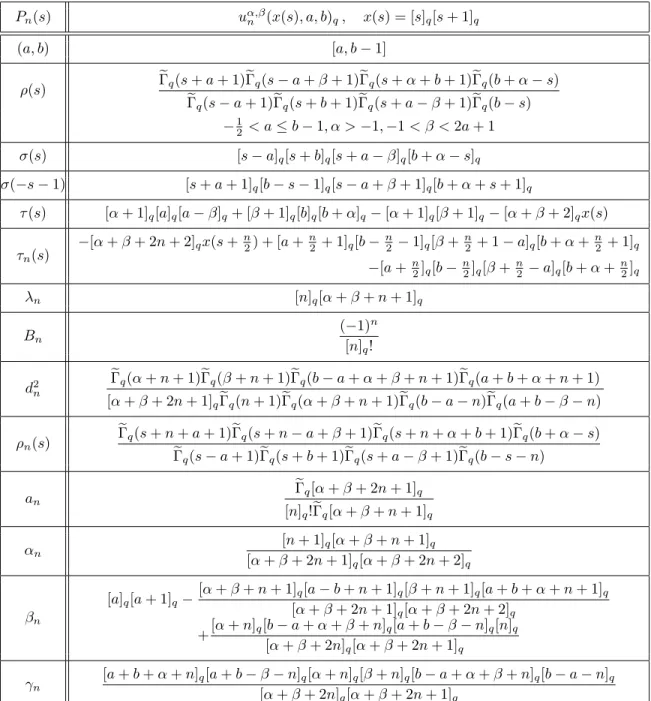
2.2. The q-Racah Polynomials euα,β
n (x(s), a, b)q
There exists another possibility to define the q-Racah polynomials as was suggested in [9, 18]. It corresponds to the function
σ(s) = [s−a]q[s+b]q[s−a+β]q[b+α+s]q,
i.e., A= 1, s1=a,s2=−b,s3 =a−β,s4=−b−α.
With this choice, we obtain a new family of polynomials ueα,βn (x(s), a, b)q that is orthogonal with
respect to the weight function
ρ(s) = eΓq(s+a+ 1)Γqe (s+a−β+ 1)
e
Γq(s+α+b+ 1)Γq(e b+α−s)eΓq(s−a+ 1)Γqe (s+b+ 1)eΓq(s−a+β+ 1)eΓq(b−s)
.
All their characteristics can be obtained exactly in the same way as before. Moreover, they can also be obtained from the corresponding characteristics of the polynomialsuα,βn (x(s), a, b)q by changingα→
−2b−α, β → 2a−β and using the properties of the functions eΓq(s), Γq(s), (a|q)n, and (a;q)n. We
summarize the main data of the polynomialseu
α,β
TABLE 2. Main Data ofq-Racah Polynomialsueα,β
n (x(s), a, b)q.
Pn(s) ueα,β
n (x(s), a, b)q, x(s) = [s]q[s+ 1]q
(a, b) [a, b−1]
ρ(s) eΓq(s+a+ 1)Γq(e s+a−β+ 1)
e
Γq(s+α+b+ 1)eΓq(b+α−s)eΓq(s−a+ 1)Γq(e s+b+ 1)Γq(e s−a+β+ 1)Γq(e b−s)
−1
2 < a≤b−1, α >−1,−1< β <2a+ 1
σ(s) [s−a]q[s+b]q[s−a+β]q[b+α+s]q
σ(−s−1) [s+a+ 1]q[b−s−1]q[s+a−β+ 1]q[b+α−s−1]q
τ(s) [2a−β+ 1]q[b]q[b+α]q−[2b+α−1]q[a]q[a−β]q−[2b+α−1]q[2a−β+ 1]q
−[2b−2a+α+β−2]qx(s)
τn(s)
−[2b−2a+α+β−2n−2]qx(s+n2)+[a+n2+1]q[b−n
2−1]q[a+
n
2+1−β]q[b−
n
2+α−1]q
−[a+n
2]q[b−
n
2]q[a+
n
2 −β]q[b−
n
2 +α]q
λn [n]q[2b−2a+α+β−n−1]q
Bn
1 [n]q!
d2
n
e
Γq(2a+n−β+1)Γeq(2b−2a+α+β−n)[2b−2a−2n−1+α+β]−1q
e
Γq(n+1)Γq(e b−a−n)eΓq(b−a−n+α)Γq(e b−a+β−n)Γqe (2b+α−n)eΓq(b−a+α+β−n)
ρn(s) Γqe (s+a+n+1)eΓq(s+a+n−β+1)
e
Γq(s+α+b+1)eΓq(b+α−s−n)Γq(e s−a+1)eΓq(s+b+1)eΓq(s−a+β+1)eΓq(b−s−n)
an
(−1)n
e
Γq[2b−2a+α+β−n]q [n]q!eΓq[2b−2a+α+β−2n]q
αn −
[n+ 1]q[2b−2a+α+β−n−1]q
[2b−2a+α+β−2n−1]q[2b−2a+α+β−2n−2]q
βn
[a]q[a+1]q+[2b−2a+α+β−n−1]q[a−b+n+1]q[2a−β+n+1]q[a−b−α+n+1]q [2b−2a+α+β−2n−1]q[2b−2a+α+β−2n−2]q
+[2b+α−n]q[b−a+α+β−n]q[b−a+β−n]q[n]q [2b−2a+α+β−2n−1]q[2b−2a+α+β−2n]q
γn −
2.2.1. The Hypergeometric Representation
For the euα,βn (x(s), a, b)q polynomials, we have the following hypergeometric representation:
e
uα,βn (x(s), a, b)q =
q−n2(4a−2b−α−β+n+1)(qa−b+1;q)n(q2a−β+1;q)n(qa−b−α+1;q)n
κ2qn(q;q)n
× 4ϕ3 q
−n, q2a−2b−α−β+n+1, qa−s, qa+s+1
qa−b+1, q2a−β+1, qa−b−α+1
q , q
!
,
(51)
or, in terms of theq-hypergeometric series (28),
e
uα,βn (x(s), a, b)q =
(a−b+ 1|q)n(2a−β+ 1|q)n(a−b−α+ 1|q)n
[n]q!
×4F3
−n,2a−2b−α−β+n+ 1, a−s, a+s+ 1
a−b+ 1,2a−β+ 1, a−b−α+ 1
q ,1
!
.
(52)
Using the Sears transformation formula (see Eq. (III.15) in [31]) we obtain the equivalent representation formulas:
e
uα,βn (x(s), a, b)q=
q−n2(2a−4b−α−β+n+1)(qa−b+1;q)n(q−2b−α+1;q)n(q−β+a−b+1;q)n
κ2qn(q;q)n
times4ϕ3 q
−n, q2a−2b−α−β+n+1, q−b−s, q−b+s+1
qa−b+1, q−2b−α+1, qa−b−β+1
q , q
! (53)
and
e
uα,βn (x(s), a, b)q=
(a−b+ 1|q)n(−2b−α+ 1|q)n(a−b−β+ 1|q)n
[n]q!
× 4F3
−n,2a−2b−α−β+n+ 1,−b−s,−b+s+ 1
a−b+ 1,−2b−α+ 1, a−b−β+ 1
q , 1
!
.
(54)
Remark: From the above formulas follows that the polynomials ueα,βn (x(s), a, b)q are multiples of the
standardq-Racah polynomials Rn(µ(qa−s);qa−b−α, qa−b−β, qa−b, qa+b|q).
Moreover, from the above hypergeometric representations we obtain the following values:
e
uα,βn (x(a), a, b)q =
(a−b+ 1|q)n(2a−β+ 1|q)n(a−b−α+ 1|q)n
[n]q!
=(q
a−b+1;q)
n(q2a−β+1;q)n(qa−b−α+1;q)n
qn2(4a−2b−α−β+n+1)κ2n
q (q;q)n
,
(55)
e
uα,βn (x(b−1), a, b)q =
(a−b+ 1|q)n(−2b−α+ 1|q)n(a−b−β+ 1|q)n
[n]q!
=(q
a−b+1;q)
n(q−2b−α+1;q)n(q−β+a−b+1;q)n
qn2(2a−4b−α−β+n+1)κ2n
q (q;q)n
.
In view of (10), we obtain the explicit formula3
e
uα,βn (x(s), a, b)q =
e
Γq(s−a+ 1)Γeq(s+b+ 1)eΓq(s−a+β+ 1)Γeq(b−s)eΓq(s+α+b+ 1)
e
Γq(s+a+ 1)Γeq(s+a−β+ 1)
×Γeq(b+α−s)
n
X
k=0
(−1)k+n[2s+ 2k−n+ 1]
qeΓq(s+k+a+ 1)Γeq(2s+k−n+ 1)
e
Γq(k+ 1)Γeq(n−k+ 1)eΓq(2s+k+ 2)eΓq(s−n+k−a+ 1)eΓq(b−s−k)
(57)
× Γeq(s+k+a−β+ 1)
e
Γq(s+k−n+α+b+ 1)eΓq(b+α−s−k)eΓq(s−n+k+b+ 1)Γeq(s−n+k−a+β+ 1)
.
From this expression follows that
e
uα,βn (x(a), a, b)q=
e
Γq(b−a)eΓq(2a−β+n+ 1)Γeq(b−a+α)
[n]!eΓq(b−a−n)Γeq(2a−β+ 1)Γeq(b−a+α−n)
,
e
uα,βn (x(b−1), a, b)q=
(−1)n
e
Γq(b−a)Γeq(2b+α)Γeq(b−a+β)
[n]!Γeq(b−a−n)eΓq(2b+α−n)Γeq(b−a+β−n)
,
(58)
which are in agreement with values (55) and (56) obtained before.
From the hypergeometric representation follows the symmetry property
e
uα,βn (x(s), a, b)q=eu
−b−a+β,b+a+α
n (x(s), a, b)q.
2.2.2. Differentiation Formulas
Next we use the differentiation formulas (21) and (23) to obtain
∆ueα,βn (x(s), a, b)q
∆x(s) =−[2b−2a+α+β−n−1]qeu
α,β
n−1(x(s+12), a+ 1 2, b−
1
2)q, (59)
[n]q[2s+ 1]que
α,β
n (x(s), a, b)q =σ(−s−1)eu
α,β
n−1(x(s+12), a+ 1 2, b−
1 2)q
−σ(s)euα,βn−1(x(s−1 2), a+
1 2, b−
1 2)q,
(60)
respectively.
Finally, formulas (24) [or (25)] and (26) lead to the following differentiation formulas:
σ(s)∇ue
α,β
n (x(s), a, b)q
[2s]q
=−[2b−2a+α+β−n−1]q [2b−2a+α+β−2n−2]q
"
τn(s)eu
α,β
n (x(s), a, b)q−[n+1]qeu
α,β
n+1(x(s), a, b)q
#
, (61)
σ(−s−1)∆ue
α,β
n (x(s), a, b)q
[2s+2]q
=−[2b−2a+α+β−n−1]q [2b−2a+α+β−2n−2]q
×
"
(τn(s)+[n]q[2b−2a+α+β−2n−2]q[2s+1]q)ue
α,β
n (x(s), a, b)q−[n+1]que
α,β
n+1(x(s), a, b)q
#
,
(62)
respectively, whereτn(s) is given in Table 2.
3
2.3. Dual Set to euα,β
n (x(s), a, b)q
To obtain the dual set toueα,βn (x(s), a, b)q, we use the same method as in the previous section.
We start from the orthogonality relation (13) for the polynomialsueα,βn (x(s), a, b)q defined by (54) and
write the dual relation
N−1
X
n=0
e
uα,βn (x(s), a, b)qeu
α,β n (x(s
0 ), a, b)q
1 d2
n
= 1
ρ(s)∆x(s−1/2)δs,s0, N =b−a, (63)
whereρandd2nare the weight function and the norm ofuenα,β(x(s), a, b)q is given in Table 2. Furthermore,
from (54) follows that the functionsue
α,β
n (x(s), a, b)q are polynomials of degreek=b−s−1 on the lattice
x(t) = [t]q[t+ 1]q, wheret=b−a−n+α+2β −1 (the proof is similar to the one presented in Sec. 2.1.4.
and we will omit it here).
To identify the dual set, let us define a new set
e
uαk0,β0(x(t), a0, b0)q =
(−1)k
e
Γq(b0−a0)eΓq(b0−a0+β0)eΓq(2b0+α0)
[k]!eΓq(b0−a0−k)eΓq(b0−a0+β0−k)Γeq(2b0+α0−k)
× 4F3
−k,2a0−2b0−α0−β0+k+ 1,−b0−t,−b0+t+ 1
a0−b0+ 1,−2b0−α0+ 1, a0−b0−β0+ 1
q ,1
!
,
(64)
where
k=b−s−1, t=b−a−n+α+β
2 −1, a
0 = α+β
2 , b
0 =b−a+α+β
2 , α
0 = 2a−β, β0 =β. (65)
Obviously they satisfy the following orthogonality relation:
b0−1
X
t=a0
e
uαk0,β0(x(t), a0, b0)qeu
α0,β0
m (x(t), a0, b0)qρ0(t)∆x(t−1/2) = (d0k)2δk,m, (66)
where nowρ0(t) and d0k are the weight function ρ and the norm dn, respectively, given in Table 2 with
the corresponding change of the parametersa, b, α, β, n, sby a0, b0, α0, β0, k, t (65).
Furthermore, with the above definition (65) for the parameters of euαk0,β0(x(t), a0, b0)q, the
hypergeo-metric function4F3 in (64) coincides with the function 4F3 in (54) and, therefore, the following relation between the polynomialseuαk0,β0(x(t), a0, b0) and ueα,βn (x(s), a, b)q holds:
e
ukα0,β0(x(t), a0, b0)q=A(eα, β, a, b, n, s)euα,βn (x(s), a, b)q, (67)
where
e
A(α, β, a, b, n, s) = (−1)
b−s−1−n
e
Γq(b−a−n)Γeq(2b+α−n)eΓq(b−a+β−n)Γeq(n+ 1)
e
Γq(b−s)eΓq(s−a+β+ 1)Γeq(s+b+α+ 1)Γeq(s−a+ 1)
.
To prove that the polynomialseuαk0,β0(x(t), a0, b0)q are the dual set toue
α,β
n (x(s), a, b)q, it is sufficient to
Let us also mention that, as in the case of the q-Racah polynomials, TTRR (16) of the polynomials
e
uαk0,β0(x(t), a0, b0)qis SODE (4) of the polynomialsue
α,β
n (x(s), a, b)q, whereas SODE (4) ofeu
α0,β0
k (x(t), a
0, b0)
q
converts into TTRR (16) of euα,βn (x(s), a, b)q, and vice versa.
To conclude this section, let us point out that there exists a simple relation connecting both polyno-mials uα,βn (x(s), a, b)q and ˜uα,βn (x(s), a, b)q [see (87) from below]. We will establish it at the end of the
next section.
3.
Connection with
6j
-Symbols of
q
-Algebra
SU
q(2)
3.1. 6j-Symbols of Quantum Algebra SUq(2)It is known (see, e.g., [21] and references therein) that the Racah coefficients Uq(j1j2j j3;j12j23) are used for the transition from the coupling scheme of three angular momentaj1, j2, j3
|j1j2(j12), j3 :jmi= X
m1,m2,m3,m12
hj1m1j2m2|j12m12ihj12m12j3m3|jmi|j1m1i|j2m2i|j3m3i
to the following ones:
|j1j2j3(j23) :jmi= X
m1,m2,m3,m23
hj2m2j3m3|j23m23ihj1m1j23m23|jmi|j1m1i|j2m2i|j3m3i,
where hjamajbmb|jabmabi denotes the Clebsch–Gordan coefficients of the quantum algebra suq(2). In
fact, we have that recoupling is given by
|j1j2(j12), j3:jmi=
X
j23
Uq(j1j2j j3;j12j23)|j1j2j3(j23) :jmi.
The Racah coefficientsU define an unitary matrix, i.e., they satisfy the orthogonality relations
X
j23
Uq(j1j2j j3;j12j23)Uq(j1j2j j3;j120 j23) =δj12,j120 , (68)
X
j12
Uq(j1j2j j3;j12j23)Uq(j1j2j j3;j12j230 ) =δj23,j230 . (69)
Usually, instead of the Racah coefficients, it is more convenient to use the 6j-symbols defined by
Uq(j1j2j j3;j12j23) = (−1)j1+j2+j3+j
q
[2j12+ 1]q[2j23+ 1]q
(
j1 j2 j12 j3 j j23
)
q
.
The 6j-symbols have the following symmetry property:
(
j1 j2 j12 j3 j j23
)
q
=
(
j3 j2 j23 j1 j j12
)
q
. (70)
Here without loss of generality, we suppose that j1 ≥j2 and j3 ≥j2; then for the momenta j23 and j12 we have the intervals
respectively. Now, in order to avoid any other restrictions on these two momenta (caused by the so-called triangle inequalities for the 6j-symbols), we assume that the following restrictions hold:
|j−j3| ≤min(j12) =j1−j2, |j−j1| ≤min(j23) =j3−j2.
3.2. 6j-Symbols and q-Racah Polynomials uα,β
n (x(s), a, b)q
Now we are ready to establish the connection of the 6j-symbols with theq-Racah polynomials. We fix the variablesass=j23that runs on the intervala≤s≤b−1, wherea=j3−j2,b=j2+j3+1. Let us put
(−1)j1+j23+j
q
[2j12+ 1]q
(
j1 j2 j12 j3 j j23
)
q
=
s
ρ(s) d2
n
uα,βn (x(s), a, b)q, (71)
whereρ(s) anddnare the weight function and the norm, respectively, of the q-Racah polynomials on the
lattice (1)uα,βn (x(s), a, b)q, and
n=j12−j1+j2, α=j1−j2−j3+j≥0, β =j1−j2+j3−j ≥0.4
To verify the above relation, we use the recurrence relation (see Eq. (5.17) in [23])
[2]q[2j23+ 2]qA−q
(
j1 j2 j12
j3 j j23−1
)
q
−([2j23]q[2j1+ 2]q−[2]q[j−j23+j1+ 1]q[j+j23−j1]q)
×([2j2]q[2j23+ 2]q−[2]q[j3−j2+j23+ 1]q[j3+j2−j23]q)
−([2j2]q[2j1+ 2]q−[2]q[j12−j2+j1+ 1]q[j12+j2−j1]q)[2j23+ 2]q[2j23]q
×[2j23+ 1]q
(
j1 j2 j12 j3 j j23
)
q
+ [2]q[2j23]qA+q
(
j1 j2 j12 j3 j j23+ 1
)
q
= 0,
(72)
where
A−q =
q
[j+j23+j1+ 1]q[j+j23−j1]q[j−j23+j1+ 1]q[j23−j+j1]q
×
q
[j2+j3+j23+ 1]q[j2+j3−j23+ 1]q[j3−j2+j23]q[j2−j3+j23]q,
A+q =
q
[j+j23+j1+ 2]q[j+j23−j1+ 1]q[j−j23+j1]q[j23−j+j1+ 1]q
×
q
[j2+j3+j23+ 2]q[j2+j3−j23]q[j3−j2+j23+ 1]q[j2−j3+j23+ 1]q.
(73)
Notice that
A−q =pσ(j23)σ(−j23), A+q =
p
σ(j23+ 1)σ(−j23−1),
4
Notice that this is equivalent to the following setting:
j1= (b−a−1 +α+β)/2, j2= (b−a−1)/2, j3 = (a+b−1)/2,
where
σ(j23) = [j23−j3+j2]q[j23+j2+j3+ 1]q[j23−j1+j]q[j+j1−j23+ 1]q,
σ(−j23−1) = [j23+j3−j2+ 1]q[j2+j3−j23]q[j23+j1−j+ 1]q[j+j1+j23+ 2]q.
Substituting (71) in (72) and simplifying the expression obtained we arrive at
[2s]qσ(−s−1)uα,βn (x(s+ 1), a, b)q+ [2s+ 2]qσ(s)unα,β(x(s−1), a, b)q
+λn[2s]q[2s+ 1]q[2s+ 2]q−[2s]qσ(−s−1)−[2s+ 2]qσ(s)
uα,βn (x(s), a, b)q= 0,
which is the difference equation for theq-Racah polynomials (4). Since uα,β0 (x(s), a, b)q= 1, relation (71) leads to
(−1)j1+j23+j
q
[2j1−2j2+ 1]q
(
j1 j2 j1−j2 j3 j j23
)
q
=
s
ρ(s) d20 ⇒
(
j1 j2 j1−j2
j3 j j23
)
q
:=
(
j1 j2 j1−j2
j3 j s
)
q
=(−1)j+j1+s
s
[j1+j+s+ 1]q![j1+j−s]q![j1−j+s]q![j3−j2+s]q!
[j−j1+s]q![j3+j2−s]q![j2−j3+s]q![j2+j3+s+ 1]q!
×
s
[2j1−2j2]q![2j2]q![j2+j3+j−j1]q!
[2j1+ 1]q![j1+j3−j2−j]q![j1−j3−j2+j]q![j1+j3−j2+j+ 1]q!
.
Furthermore, substituting the valuess=aand s=b−1 in (71) and using (41) we find
(
j1 j2 j12 j3 j j3−j2
)
q
= (−1)j12+j3+j
×
s
[j12+j3−j]q![2j2]q![j12+j3+j+ 1]q![2j3−2j2]q![j2−j1+j12]q!
[j1−j2+j3−j]q![j1+j2−j12]q![j1−j2+j3+j+ 1]q!
×
s
[j1+j2−j3+j]q![j1−j2+j12]q![j3−j12+j]q!
[2j3+ 1]q![j3−j1−j2+j]q![j12−j3+j]q![j1+j2+j12+ 1]q!
(74)
and
(
j1 j2 j12 j3 j j2+j3
)
q
= (−1)j1+j2+j3+j
×
s
[2j2]q![j12−j3+j]q![j2−j1+j3+j]q![2j3]q![j1+j2+j3−j]q!
[j1+j2−j12]q![j1−j2−j3+j]q![j3−j12+j]q!
×
s
[j2−j1+j12]q![j1−j2+j12]q![j1+j2+j3+j+ 1]q!
[2j2+ 2j3+ 1]q![j12+j3−j]q![j1+j2+j12+ 1]q![j12+j3+j+ 1]q!
,
which are in agreement with the results of [21].
Relation (71) allows us to obtain several recurrence relations for the 6j-symbols of the quantum algebraSUq(2) by using the properties of the q-Racah polynomials. So, TTRR (16) gives
[2j12]qAe+q (
j1 j2 j12+ 1
j3 j j23
)
q
+ [2j12+ 2]qAe−q (
j1 j2 j12−1
j3 j j23
)
q
−[2j12]q[2j12+ 1]q[2j12+ 2]q [j23]q[j23+ 1]q−[j3−j2]q[j3−j2+ 1]q
+ [2j12]q
×[j1−j2+j12+ 1]q[j12−j1−j2]q[j12+j3−j+ 1]q[j12+j3+j+ 2]q−[2j12+ 2]q
×[j12−j3+j]q[j1+j2+j12+ 1]q[j3−j12+j+ 1]q[j2−j1+j12]q
(
j1 j2 j12
j3 j j23
)
q
= 0,
(76)
where
e
A−q =
q
[j2−j1+j12]q[j1−j2+j12]q[j12−j3+j]q[j12+j3−j]q[j1+j2+j12+ 1]q
×
q
[j12+j3+j+ 1]q[j1+j2−j12+ 1]q[j3−j12+j+ 1]q,
e
A+q =
q
[j2−j1+j12+ 1]q[j1−j2+j12+ 1]q[j12−j3+j+ 1]q[j12+j3−j+ 1]q
×q[j1+j2+j12+ 2]q[j12+j3+j+ 2]q[j1+j2−j12]q[j3−j12+j]q.
(77)
Expressions (42) and (43) yield
p
σ(j23+ 1)
(
j1 j2 j12 j3 j j23+ 1
)
q
+pσ(−j23−1)
(
j1 j2 j12 j3 j j23
)
q
= [2j23+ 2]q
q
[j2−j1+j12]q[j1−j2+j12+ 1]q
(
j1+12 j2− 12 j12 j3 j j23+ 12
)
q
(78)
and
p
σ(−j23−1)
(
j1+12 j2− 12 j12
j3 j j23+ 12
)
q
+pσ(j23)
(
j1+12 j2−12 j12
j3 j j23−12
)
q
= [2j23+ 1]q
q
[j12−j1+j2]q[j12+j1−j2+ 1]q
(
j1 j2 j12
j3 j j23
)
q
,
(79)
respectively, whereas the differentiation formulas (44)–(45) give
[2j12+ 2]qA−q
(
j1 j2 j12 j3 j j23−1
)
q
+ [2j23]qAe+q (
j1 j2 j12+ 1 j3 j j23
)
q
+σ(j23)[2j12+ 2]q+ [j1−j2+j12+ 1]q[2j23]qΛ(j12, j23, j1, j2)
(
j1 j2 j12 j3 j j23
)
q
and
[2j12+ 2]qA+q
(
j1 j2 j12
j3 j j23+ 1
)
q
−[2j23+ 2]qAe+q (
j1 j2 j12+ 1
j3 j j23
)
q
+
[2j12+ 2]qσ(−j23−1)−[2j23+ 2]q[j1−j2+j12+ 1]q(Λ(j12, j23, j1, j2)
+ [j12−j1+j2]q[2j12+ 2]q[2j23+ 1]q)
(
j1 j2 j12 j3 j j23
)
q
= 0,
(81)
respectively, whereA±q are given by (73), Ae±q by (77), and
Λ(j12, j23, j1, j2) =σ
−j12+j1−j2
2 −1
−σ
−j12+j1−j2 2
−[2j12+ 2]q
j23+j12−j1+j2 2
q
j23+j12−j1+j2
2 + 1
q
.
Using the hypergeometric representations (35) and (37) we obtain the representation of the 6j-symbols in terms of theq-hypergeometric function5 (28)
(
j1 j2 j12
j3 j j23
)
q
= (−1)j12+j23+j2+j [2j2]q!
[j1−j2+j3−j]q![j1−j2+j3+j+ 1]q!
×
s
[j1+j+j23+ 1]q![j1+j−j23]q![j1−j+j23]q![j3−j2+j23]q!
[j−j1+j23]q![j3+j2−j23]q![j2−j3+j23]q![j2+j3+j23+ 1]q!
×
s
[j12−j1+j2]q![j12+j1−j2]q![j3+j−j12]q![j3+j12−j]q![j3+j12+j+ 1]q!
[j12−j3+j]q![j1+j2+j12+ 1]q![j1+j2−j12]q!
×4F3
j1−j2−j12, j1−j2+j12+ 1, j3−j2−j23, j23+j3−j2+ 1 −2j2, j1−j2+j3−j+ 1, j1−j2+j3+j+ 2
q ,1
!
and
(
j1 j2 j12 j3 j j23
)
q
= (−1)j1+j23+j[2j2]q![j2+j3−j1+j]q!
[j1−j2−j3+j]q!
×
s
[j1+j+j23+ 1]q![j1+j−j23]q![j1−j+j23]q![j3−j2+j23]q!
[j−j1+j23]q![j3+j2−j23]q![j2−j3+j23]q![j2+j3+j23+ 1]q!
×
s
[j12−j1+j2]q![j12+j1−j2]q![j12−j3+j]q!
[j1+j2+j12+ 1]q![j1+j2−j12]q![j3+j−j12]q![j12+j3−j]q![j3+j12+j+ 1]q!
×4F3
j1−j2−j12, j1−j2+j12+ 1,−j3−j2+j23,−j23−j3−j2−1 −2j2, j1−j2−j3+j+ 1, j1−j2−j3−j
q , 1
!
.
5
Notice that values (74) and (75) immediately follow from the above representations.
Notice also that the above formulas give two alternative explicit formulas for computing the 6j -symbols.
The third explicit formula follows from (40):
(
j1 j2 j12 j3 j j23
)
q
=
s
[j23+j2−j3]q![j23+j2+j3+ 1]q![j23+j−j1]q![j2+j3−j23]q!
[j23+j3−j2]q![j23+j1−j]q![j23+j1+j+ 1]q![j1+j−j23]q!
×
s
[j12−j1+j2]q![j1−j2+j12]q![j1+j2−j12]q![j3−j12+j]q!
[j12−j3+j]q![j12+j3−j]q![j1+j2+j12+ 1]q![j12+j3+j]q!
×
j12−j1+j2
X
k=0
(−1)k+j1+j23+j[2k+j
1−j2−j12+ 2j23+ 1]q[k+j23+j3−j2]q!
[k]q![j12−j1+j2−k]q![2j3+ 1 +k]q![k+j23+j1−j12−j3]q!
×[2j23+k−j12+j1−j2]q![k+j23+j1−j]q![k+j23+j1+j+ 1]q![j1+j−j23−k]q! [k+j23+j1−j12+j3+ 1]q![k+j23+j−j2−j12]q![j2+j3−j23+ 1−k]q!
.
To conclude this section, let us point out that the orthogonality relations (68) and (69) lead to the orthogonality relations for the Racah polynomialsuα,βn (x(s), a, b)q (35) and their duals uα
0,β0
k (x(t), a
0, b0)
q,
respectively, and also that relation (50) between theq-Racah and dualq-Racah polynomials corresponds to the symmetry property (70).
3.3. 6j-Symbols and Alternative q-Racah Polynomials euα,β
n (x(s), a, b)q
In this section, we provide the same comparative analysis but for the alternativeq-Racah polynomials
e
uα,βn (x(s), a, b)q.
We again choose s=j23 that runs on the interval [a, b−1], a=j3−j2,b=j2+j3+ 1. In this case, the connection is given by the formula
(−1)j12+j3+j
q
[2j12+ 1]q
(
j1 j2 j12
j3 j j23
)
q
=
s
ρ(s) d2
n
e
uα,βn (x(s), a, b)q, (82)
where ρ(s) and dn are the weight function and the norm, respectively, of the alternativeq-Racah
poly-nomialseu
α,β
n (x(s), a, b)q (see Sec. 2.2.) on the lattice (1) and
n=j1+j2−j12, α=j1−j2−j3+j≥0, β =j1−j2+j3−j≥0.
In view of the above relations, one sees that SODE (4) for the polynomialsueα,βn (x(s), a, b)q converts
respectively. If we now put n= 0, i.e.,j12=j1+j2, we obtain the value
(
j1 j2 j1+j2
j3 j j23
)
q
:=
(
j1 j2 j1+j2
j3 j s
)
q
= (−1)j1+j2+j3+j
s
[2j1]q![2j2]q![j1+j2+j3+j+ 1]q![j1+j2−j3+j]q!
[2j1+ 2j2+ 1]q![−j1−j2+j3+j]q![j2+j3+s+ 1]q!
×
s
[s−j1+j]q![s−j2+j3]q!
[j1+j−s]q![j1−j+s]q![j1+j+s+ 1]q![j2+j3−s]q![j2−j3+s]q!
.
Expressions (59) and (60) yield
p
ς(j23+ 1)
(
j1 j2 j12 j3 j j23+ 1
)
q
−pς(−j23−1)
(
j1 j2 j12 j3 j j23
)
q
= [2j23+ 2]q
q
[j1+j2−j12]q[j1+j2+j12+ 1]q
(
j1−12 j2− 12 j12 j3 j j23+ 12
)
q
(83)
and
p
ς(−j23−1)
(
j1−12 j2− 12 j12 j3 j j23+ 12
)
q
−pς(j23)
(
j1−12 j2−12 j12 j3 j j23− 12
)
q
= [2j23+ 1]q
q
[j1+j2−j12]q[j1+j2+j12+ 1]q
(
j1 j2 j12 j3 j j23
)
q
,
(84)
respectively, where
ς(j23) = [j23−j3+j2]q[j23+j2+j3+ 1]q[j23−j1+j+ 1]q[j+j1+j23+ 1]q,
ς(−j23−1) = [j23+j3−j2+ 1]q[j2+j3−j23]q[j23+j1−j+ 1]q[j+j1−j23]q.
Differentiation formulas (61)–(62) give
[2j12]qA−q
(
j1 j2 j12 j3 j j23−1
)
q
−[2j23]qAe−q (
j1 j2 j12−1 j3 j j23
)
q
−ς(j23)[2j12]q+ [j1+j2+j12+ 1]q[2j23]qΛ(e j12, j23, j1, j2)
(
j1 j2 j12
j3 j j23
)
q
= 0 (85)
and
[2j12]qA+q
(
j1 j2 j12
j3 j j23+ 1
)
q
+ [2j23+ 2]qAe−q (
j1 j2 j12−1
j3 j j23
)
q
−[2j12]qς(−j23−1)−[2j23+ 2]q[j1+j2+j12+ 1]q
e
Λ(j12, j23, j1, j2)
+[j1+j2−j12]q[2j12]q[2j23+ 1]q)
(
j1 j2 j12 j3 j j23
)
q
= 0,
respectively, whereA±q are given by (73), Ae±q by (77), and
e
Λ(j12, j23, j1, j2) =ς
j12−j1−j2
2 −1
−ς
j12−j1−j2 2
−
[2j12]q
j23+
j1+j2−j12 2
q
j23+
j1+j2−j12
2 + 1
q
.
If we now use the hypergeometric representations (52) and (54), we obtain two new representations of the 6j-symbols in terms of the q-hypergeometric function (28)
(
j1 j2 j12 j3 j j23
)
q
= (−1)j12+j3+j[2j2]q![j1+j2−j3+j]q!
[j3−j2−j1+j]q!
×
s
[j−j1+j23]q![j3−j2+j23]q!
[j1+j+j23+ 1]q![j1+j−j23]q![j2−j3+j23]q![j2+j3+j23+ 1]q![j1−j+j23]q!
×
s
[j3−j12+j]q![j12+j3−j]q![j3+j12+j+ 1]q![j1−j2+j12+ 1]q!
[j3+j2−j23]q![j1+j2−j12]q![j2−j1+j12]q![j12−j3+j]q![j1+j2+j12+ 1]q!
×4F3
j12−j1−j2,−j1−j2−j12−1, j3−j2−j23, j23+j3−j2+ 1 −2j2, j3−j1−j2+j+ 1, j3−j1−j2−j
q , 1
!
and
(
j1 j2 j12 j3 j j23
)
q
= (−1)j1+j23+j[2j2]q![j1+j2+j3+j]q![j1+j2+j3−j]q!
p
[j3+j2−j23]q![j1+j2−j12]q!
×
s
[j−j1+j23]q![j3−j2+j23]q!
[j1+j+j23+ 1]q![j1+j−j23]q![j2−j3+j23]q![j2+j3+j23+ 1]q![j1−j+j23]q!
×
s
[j12−j3+j]q![j12+j1−j2+ 1]q!
[j3−j12+j]q![j12+j3−j]q![j1+j2+j12+ 1]q![j2−j1+j12]q![j3+j12+j+ 1]q!
×4F3
j12−j1−j2,−j1−j2−j12−1,−j3−j2−j23−1, j23−j3−j2 −2j2, −j1−j2−j3−j, j−j1−j2−j3
q , 1
!
.
Notice that values (74) and (75) also follow from the above representations.
Finally, from (57) follows
(
j1 j2 j12
j3 j j23
)
q =
s
[j23+j1+j+ 1]q![j1−j23+j]q![j2−j3+j23]q![j2+j3+j23+ 1]q!
[j23−j2+j3]q![−j1+j23+j]q![−j12+j3+j]q![j1+j2+j12+ 1]q!
×
s
[j1+j23−j]q![j2+j3−j23]q![j1+j2−j12]q![−j1+j2+j12]q!
[−j3+j+j12]q!−1[j12+j3+j+ 1]q!−1[j1−j2+j12]q!−1
×
j1+j2−j12
X
l=0
(−1)l+j1+j2+j3+j[2j
23+ 2l−j1−j2+j12+ 1]q
[l]q![j1+j2−j12−l]q![2j23+l+ 1]q![j23−j1−j2+j12+l+j2−j3]q![j2+j3−j23−l]q!
× [2j23+l−j1−j2+j12]q![j23+l−j2+j3]q![−j1+j+j23+l]q!
[l+j12−j2+j+j23+ 1]q![j1+j−j23−l]q![−j1+j12+j3+j23+l+ 1]q![−j2+j12−j+j23+l]q!
.
To conclude this section, let us point out that the orthogonality relations (68) and (69) lead to the orthogonality relations for the alternative Racah polynomials euα,βn (x(s), a, b)q (52) and their duals
e
uαk0,β0(x(t), a0, b0)q(64), respectively, and relation (67) between theq-Racah and dualq-Racah polynomials
corresponds to the symmetry property (70).
3.4. Connection between euα,βk (x(s), a, b)q and uα,βn (x(s), a, b)q
Let us obtain the formula connecting the two familiesueα,βk (x(s), a, b)q and uα,βn (x(s), a, b)q.
In fact, Eqs. (71) and (82) suggest the following relation between both Racah polynomials
e
uα,βk (x(s), a, b)q and uα,βn (x(s), a, b)q:
e
uα,βb−a−1−n(x(s), a, b)q= (−1)s−a−n
× Γeq(s−a+β+ 1)Γeq(b+α−s)eΓq(b+α+ 1 +s)Γeq(a+b−β−n)
e
Γq(s+a−β+ 1)Γeq(α+ 1 +n)Γeq(β+ 1 +n)Γeq(a+b+α+ 1 +n)
uα,βn (x(s), a, b)q.
(87)
To prove this, it is sufficient to substitute the above formula into the difference equation (4) of the polynomialseuα,βn (x(s), a, b)q.
After some straightforward computations, the resulting difference equation converts into the corre-sponding difference equation for the polynomials uα,βn (x(s), a, b)q.
Notice that from this relation follows that
4F3
a−b+n+ 1, a−b−α−β−n, a−s, a+s+ 1 a−b+ 1,2a−β+ 1, a−b−α+ 1
q , 1
!
= (β+ 1|q)s−a(b+α+a+ 1|q)s−a (2a−β+ 1|q)s−a(a−b−α+ 1)s−a4
F3
−n, α+β+n+ 1, a−s, a+s+ 1
a−b+ 1, β+ 1, a+b+α+ 1
q , 1
!
.
This provides the following identity for terminating the4φ3 basic series (n, N −n−1, k= 0,1,2, . . .):
4ϕ3
qn−N+1, q−n−N+1A−1B−1, q−k, q−kD q1−N, q−2kDB−1, q1−NA−1
q , q
!
= q −kN
AkBk
(qB;q)k(qN−2kDA;q)k
(q−2kDB−1;q)
k,(q1−NA−1;q)k4
ϕ3 q
−n, ABqn, q−k, q−kD
q1−N, qB, qN−2kDA
q , q
!
4.
Conclusions
Here we have provided a detailed study of two kinds of Racah q-polynomials on the lattice x(s) = [s]q[s+ 1]qand also their comparative analysis with the Racah coefficients or 6j-symbols of the quantum
algebraUq(su(2)).
To conclude the paper, we will briefly discuss the relation of the q-Racah polynomials to the repre-sentation theory of the quantum algebra Uq(su(3)). In [9] (see § 5.5.3 therein) it was shown that the
transformation between two different bases (λ, µ) of the irreducible representation of the classical (not q) algebra su(3) corresponding to the reductions su(3)⊃su(2)×u(1) and su(3) ⊃u(1)×su(2) of the su(3) algebra in two different subalgebras su(2) is given in terms of the Weyl coefficients that are, up to a sign (phase), the Racah coefficients of the algebra su(2). The same statement can be made in the case of the quantum algebra suq(3) [32, 33]. The Weyl coefficients of the transformation between two
bases of the irreducible representation (λ, µ) corresponding to the reductions suq(3) ⊃ suq(2)×uq(1)
andsuq(3)⊃uq(1)×suq(2) of the quantum algebrasuq(3) in two different quantum subalgebras suq(2)
coincide (up to a sign) with the q-Racah coefficients ofsuq(2).
In fact, the Weyl coefficients satisfy certain difference equations that are equivalent to the differen-tiation formulas for theq-Racah polynomials uα,βn (x(s), a, b)q and eu
α,β
n (x(s), a, b)q; so, following the idea
of [9] (see§ 5.5.3 therein), we can assure that the main properties of theq-Racah polynomials are closely related to the representations of the quantum algebraUq(su(3)). Finally, let us point out that the same
assertion can be made but with the noncompact quantum algebra Uq(su(2,1)). This will be carefully
done in a forthcoming paper.
The results obtained can be used in models of photon–atom interactions which employ polynomial Hamiltonians. In these models, structures like the q-analogs of Racah polynomials naturally appear in quantum optics.
Acknowledgments
This research has been supported by the DGES grant BFM 2003-06335-C03 (RAN, RCS) and the PAI grant FQM-0262 (RAN). Yu. F. S. is thankful to the Russian Foundation for Basic Research for partial support under Project No. 02-01-00668.
References
1. I. A. Malkin and V. I. Man’ko,Dynamic Symmetries and Coherent States of Quantum Systems[in Russian], Nauka, Moscow (1979).
2. J Guerrero, V. I. Man’ko, G. Marmo, and A. Simoni, “Geometrical aspects of the Lie group representation and their optical applications,”J. Russ. Laser Res.,23, 49–80 (2002).
3. B. Gruber, Yu. F. Smirnov, and Yu. I. Kharitonov, “Quantum algebra Uq(gl(3)) and nonlinear
optics,”J. Russ. Laser Res.,24, 56–68 (2003).
4. L. D. Landau and E. M. Lifshits, Quantum Mechanics. Nonrelativistic Theory [in Russian], Fiz-matlit, Moscow (2002).
![TABLE 2. Main Data of q-Racah Polynomials u e α,βn (x(s), a, b) q . P n (s) u e α,βn (x(s), a, b) q , x(s) = [s] q [s + 1] q (a, b) [a, b − 1] ρ(s) e Γ q (s + a + 1)eΓ q (s + a − β + 1) e](https://thumb-us.123doks.com/thumbv2/123dok_es/5819402.146098/17.918.129.756.253.979/table-main-data-racah-polynomials-βn-γ-eγ.webp)
