How well can the New Open Economy
Macroeconomics explain the exchange
rate and current account?
Paul R. Bergin
a,b,*
aDepartment of Economics, University of California, One Shields Avenue, Davis, CA 95616-8578, USA b
NBER, USA
Abstract
This paper advances the New Open Economy Macroeconomic literature in an empirical direction, esti-mating and testing a two-country model. Fit to U.S. and G7 data, the model performs moderately well for the exchange rate and current account. Results offer guidance for future theoretical work. Parameter esti-mates lend support to the assumption of local currency pricing. Estiesti-mates are found for key parameters com-monly calibrated in the theoretical literature, such as the elasticity of substitution between home and foreign composite goods, and the response of a country’s risk premium to the net foreign asset position. Results also indicate that deviations from interest rate parity are not closely related to monetary policy shocks, as recently hypothesized, but that these deviations are strongly related to shifts in the current account. 2006 Elsevier Ltd. All rights reserved.
JEL classification:F41
Keywords:New Open Economy Macroeconomics; Estimation; Interest rate parity
1. Introduction
International macroeconomists increasingly have come to rely upon a class of models known as New Open Economy Macroeconomics (NOEM), characterized by microeconomic founda-tions in combination with nominal rigidities. While theoretical work in the NOEM literature
* Department of Economics, University of California, Davis, One Shields Avenue, Davis, CA 95616-8578, USA. Tel.:þ1 530 752 8398; fax:þ1 530 752 9382.
E-mail address:[email protected]
0261-5606/$ - see front matter2006 Elsevier Ltd. All rights reserved. doi:10.1016/j.jimonfin.2006.04.001
has grown rapidly, there has been comparatively little work done on empirical dimensions.1 This has not been for a lack of interest, as it generally is agreed that if we are to trust these models for policy analysis, we should have some degree of confidence that they accurately re-flect basic features of the economy. However, the macroeconomic models developed recently are sufficiently complex that estimating and testing them econometrically calls for new tools. This paper advances the NOEM literature in an empirical direction, estimating and testing
a two-country model by maximum likelihood methods.2This estimation provides several
re-sults that could be useful in guiding future theoretical work.
The empirical record for earlier classes of macroeconomic models is very mixed. This is es-pecially true with regard to the exchange rate and the current account, key variables for open economy macroeconomics. The current account dynamics of many countries have proved quite
difficult to explain in terms of macroeconomic models using present value tests.3And in a
clas-sic result,Meese and Rogoff (1983) showed that a range of macroeconomic models were
un-able to beat a random walk in forecasting the nominal exchange rate. Exchange rate movements have proved so problematic that some recent research has recommended abandoning the
at-tempt of explaining them in terms of macroeconomic models (seeFlood and Rose, 1999).
As a result, it is becoming a familiar practice in NOEM studies to introduce exchange rate movements in a manner other than macroeconomic fundamentals. This often is done by adding
an extra term to the uncovered interest rate parity condition (UIP) in the macro model.4Such
a term is motivated by well-documented empirical evidence of strong deviations from UIP,5and
it can be interpreted in a number of different ways:Obstfeld and Rogoff (2002)derive such
a term as a currency risk premium which is associated with monetary policy actions; Mark
and Wu (1998)andJeanne and Rose (2002)derive it as a reflection of noise traders and a dis-tribution of exchange rate expectations.
In response to the controversy regarding macro models as explanations for the exchange rate and current account, this paper will pay special attention to these two variables. In particular, a maximum likelihood approach is adapted for estimating and evaluating a two-country NOEM model. The U.S. is used as one of these countries, and an aggregate of the remaining G7 is used as the other country. The model is fit to five data series: the exchange rate, current account, output growth, inflation, and interest rate deviations between the two countries. Data are quar-terly from 1973:1 to 2000:4.
The model shares many features common in NOEM models, including monopolistically competitive firms, sluggish price setting, capital accumulation subject to adjustment costs, and monetary policy in the form of interest rate setting rules. The procedure will estimate
1
In open economy work, seeBergin (2003)andGhironi et al. (2003); in closed economy work, seeIreland (1997, 2001), Kim (2000), Lubik and Schorfheide (2004), andSmets and Wouters (2002).
2
The current exercise goes beyond the initial empirical work inBergin (2003)in important ways. In general terms, the model here is better suited to current questions raised in the theoretical literature, which are discussed in detail later in the paper. First, the model develops a means to allow multiple types of price stickiness to coexist, and so it can es-timate the share of each type. Second, it uses a more general form of household preferences, to see if the eses-timated parameters support common assumptions in the theoretical literature regarding these preferences. Third, it does not as-sume that interest rate parity holds. The exercise also is improved on technical grounds, by ensuring stationarity of the wealth distribution and by allowing monetary policy authorities to respond to economic conditions. A final distinction is that instead of a small open economy, a two-country environment is modeled here, which is better suited to analyzing issues of the U.S. economy.
3For example, seeSheffrin and Woo (1990), Ghosh (1995), andBergin and Sheffrin (2000). 4
For examples, seeMcCallum and Nelson (1999, 2000), Kollmann (2001, 2002), andJeanne and Rose (2002). 5
various deep parameters of interest in the theoretical literature. There will be five shocks to the system, including technology, monetary policy, consumption tastes, and the share of home bias in preferences; the fifth shock will be to the interest rate parity condition. The estimation pro-cedure will also estimate the degree of correlation between the four structural shocks and the deviations from UIP.
Results indicate that the model as equipped above is able to explain the exchange rate and current account to some degree, in that it can beat a random walk in one-step ahead in-sample predictions. It is not able to beat a standard vector autoregression in terms of predictions for the exchange rate and current account, although the overall fit of the model is superior to the VAR when the latter is appropriately penalized for its larger set of free parameters.
Parameter estimates are able to help address some current controversies in the theoretical
NOEM literature. One such controversy deals with the nature of price stickiness. WhileBetts
and Devereux (2000)have argued that stickiness in the local currency of the buyer improves the
model’s ability to explain certain stylized facts regarding the exchange rate,Obstfeld and
Rog-off (2000)have argued the opposite case. The model here permits both types of price stickiness to coexist, where the share is a parameter that can be estimated. Estimates indicate that a very high degree of local currency pricing is needed to successfully explain exchange rate move-ments in this data set. A second controversy regards the nature of household preferences, in particular, whether there is a unitary elasticity of substitution between home and foreign goods. This highly convenient assumption has become common practice in the theoretical literature, although it stands in contrast to empirical studies based on micro-level evidence. The estimates of this elasticity in the present paper offer empirical evidence from macro-level data which support this common practice in the theoretical literature. Further, it has become common prac-tice in NOEM models to impose stationarity on the net foreign asset position by specifying a country premium on interest rates, where this premium has a positive relationship to net for-eign debt. The estimation exercise here offers an estimate for the parameter characterizing this positive relationship, which could prove useful as a basis for calibrations in future theoretical work.
Estimates also offer some new insights into the nature of deviations from uncovered interest rate parity (UIP). Results indicate that UIP deviations are not very closely related to monetary policy actions, contrary to a hypothesis in some theoretical NOEM work. However, these de-viations are very highly correlated with shocks to marginal utility (taste shocks). Surprisingly, it appears that UIP shocks are even more important for explaining movements in the current ac-count than the exchange rate. This may indicate that current acac-count movements are determined in large part by financial shocks, which affect capital account flows, and thereby force current account adjustments through the balance of payments identity. This idea is quite different from the usual NOEM theory of the current account, as simply reflecting optimal saving and invest-ment decisions, and it suggests a useful avenue for future research.
2. The model
2.1. General features
Consider a two-country world, where the countries will be denoted home and foreign, and
the population of home is fractionnof the world total. Each country has a representative
house-hold and a representative firm, and each country has a distinct continuum of intermediate goods
subscript. All variables will be written in per capita terms. Steady state levels will be indicated by overbars.
2.2. Market structure
Final goods in this economy (Yt) are produced by aggregating over a continuum of
inter-mediate home goods indexed by i˛[0, 1] along with aggregating over a continuum of
im-ported foreign goods indexed by j˛[0, 1]. The aggregation technology for producing final
goods is:
Yt¼
½
q 1m
tY
m1
m
Ht þ ð1qtÞ 1
mY m1
m
Ft
m m1
; ð1Þ
where
YHt¼ Z 1
0 yHtðiÞ
1 1þndi
!1þn
ð2Þ
YFt¼ Z 1
0 yFtðjÞ
1 1þndj
!1þn
: ð3Þ
HereYHtrepresents an aggregate of the home goods sold in the small open economy, andYFt
is an aggregate of the imported foreign goods, where lower case counterparts with indexes
rep-resent outputs of the individual firms. Note that the share parameter,qt, is subject to stochastic
shocks.
Final goods producers behave competitively, maximizing profit each period:
p1t¼maxPtYtPHtYHtPFtYFt; ð4Þ
wherePtis the overall price index of the final good,PHtis the price index of home goods, and
PFtis the price index of foreign goods, all denominated in the home currency. It is assumed that
fractionhof firms (indexedi¼0,.h) exhibit local currency pricing, that is, they set the price
of goods in the currency of the buyer. It is assumed that the remaining fraction 1hof firms
(indexedi¼h,.1) exhibit producer currency pricing, that is, they set the price of goods in
their own currency.
The price indexes may be defined:
Pt¼
qtP1Htmþ ð1qtÞP1Ftm 1
1m; ð5Þ
where
PHt¼ 0 @Z h
0 pHtðiÞ
1
ndiþ
Z 1
h pHtðiÞ
1
ndi
1 A
n
PFt¼ 0 @Z h
0 pFtðjÞ
1
ndjþ
Z 1
h spFtðjÞ
1
ndj
1 A
n
; ð7Þ
and where lower case counterparts again represent the prices set by individual firms. The
nom-inal exchange rate (st) is the home currency price of one unit of the world currency. And the
price index of home exports may be expressed:
PHt¼
0 @Z h
0
pHtðjÞ1ndjþ
Z 1
h 1 st
pHtðjÞ1ndj
1 A
n
: ð8Þ
Given the aggregation functions above, demand will be allocated between home and foreign goods according to:
YHt¼qtYtðPt=PHtÞ
m
ð9Þ
YFt¼ ð1qtÞYtðPt=PFtÞ
m
; ð10Þ
with demands for individual goods:
yHtðiÞ ¼YHtðpHtðiÞ=PHtÞ
ð1þnÞ=n
ð11Þ
yFtðjÞ ¼YFtðpFtðjÞ=PFtÞ
ð1þnÞ=n
for j¼0;.;h ð12Þ
yFtðjÞ ¼YFtðstpFtðjÞ=PFtÞð1þnÞ=n for j¼h;.;1: ð13Þ
Analogous conditions apply to the foreign country.
2.3. Firm behavior
The firms rent capital (Kt) at the real rental ratert, and hire labor (Lt) at the nominal wage
rateWt. It is assumed that it is costly to reset prices because of quadratic menu costs. The
prob-lem for the local currency pricing (i¼0,.h) firms may be summarized:
maxEt
XN
n¼0
rt;tþnpH;tþnðiÞ; ð14Þ
where
pHtðiÞ ¼pHtðiÞyHtðiÞ þstpHtðiÞ
1
n n
yHtðiÞ PtrtKt1ðiÞ WtLtðiÞ PtACHtðiÞ
stPtACHtðiÞ ð15Þ
s:t: ACHtðiÞ ¼
jP 2
ðpHtðiÞ pHt1ðiÞÞ 2
PtpHt1ðiÞ
ACHtðiÞ ¼jP
2
p
HtðiÞ pHt1ðiÞ
2
PtpHt1ðiÞ
1
n n
yHtðiÞ ð17Þ
zðiÞt¼AtKt1ðiÞaLtðiÞ1a ð18Þ
zðiÞt¼yHtðiÞ þ
1
n n
yHtðiÞ; ð19Þ
and subject to the demand functions foryHt(i) andy*Ht(i) above. HereAtrepresents technology
common to all production firms in the country, and it is subject to shocks. Lastly,rt,tþnis the
pricing kernel used to value random datetþnpayoffs. Since firms are assumed to be owned by
the representative household, it is assumed that firms value future payoffs according to the
household’s intertemporal marginal rate of substitution in consumption, sort,tþn¼bnU0C,tþn/
U0C,t, where UC,0 tþn is the household’s marginal utility of consumption in period tþn. The
problem for the producer currency pricing firms (i¼h.1) is identical, except thatpH*t(i) is
in units of home currency and Eq.(15)is replaced by:
pHtðiÞ ¼pHtðiÞyHtðiÞ þpHtðiÞ
1
n n
yHtðiÞ Ptrt1Kt1ðiÞ WtLtðiÞ PtACHtðiÞ
PtACHtðiÞ:
This problem implies an optimal trade-off between capital and labor inputs that depend on the relative cost of each:
PtrtKt1ðiÞ ¼
a
1aWtLtðiÞ: ð20Þ
The optimal price setting rule for domestic sales of all home firms (i¼0,., 1) is:
1þv
v
Ptrt
PHtaAtðLtðiÞ=Kt1ðiÞÞ ð1aÞþ
jP 2
ðpHtðiÞ pHt1ðiÞÞ2 PHtpHt1ðiÞ
pHtðiÞ
PHt !
YHt
yHtðiÞ
pHtðiÞ
PHt ð1þ2n
n Þ
þjP
2Et
r t;tþiþ1
rt;tþi p2
Htþ1ðiÞ p2
HtðiÞ
1
yHtþ1ðiÞ
yHtðiÞ
jP
pHtðiÞ
pHt1ðiÞ
1
þ1¼0:
ð21Þ
The optimal price setting rule for exports for local currency pricing firms (i¼0,.,h) is:
1þv
v
Ptrt
stPHtaAtðLtðiÞ=Kt1ðiÞÞ ð1aÞþ
jP 2
pHtðiÞ pHt1ðiÞ2
P
HtpHt1ðiÞ
p
HtðiÞ
P Ht
! YHt
y HtðiÞ
p
HtðiÞ
PHt ð1þ2n
n Þ
þjP
2Et
r t;tþiþ1
rt;tþi
p2 Htþ1ðiÞ p2
HtðiÞ
1
stþ1
st
yHtþ1ðiÞ yHtðiÞ
jP
p
HtðiÞ
pHt1ðiÞ
1
and the optimal price for exports by producer currency pricing firms (i¼h,., 1) is:
1þv
v
Ptrt1
stPHtaAtðLtðiÞ=Kt1ðiÞÞð1 aÞþ
jP 2
p
HtðiÞ pHt1ðiÞ
2
stPHtpHt1ðiÞ
p
HtðiÞ
stPHt !
YHt
y HtðiÞ
pHtðiÞ
stPHt ð1þ2n
n Þ
þjP
2Et
r t;tþiþ1
rt;tþi
p2 Htþ1ðiÞ p2
HtðiÞ
1
y
Htþ1ðiÞ y
HtðiÞ
jP
pHtðiÞ
p Ht1ðiÞ
1
þ1¼0: ð23Þ
2.4. Household behavior
The household derives utility from consumption (Ct), and supplying labor (Lt) lowers utility.
For simplicity, real money balances (Mt/Pt) are also introduced in the utility function, wherePt
is the overall price level. The household discounts future utility at the rate of time preferenceb.
Preferences are additively separable in these three arguments, and preferences for consumption
are subject to preference shocks (tt).
Households derive income by selling their labor at the nominal wage rate (Wt), renting
cap-ital to firms at the real rental rate (rt), receiving real profits from the two types of firms (p1tand
p2t), and from government transfers (Tt). In addition to money, households can hold two types
of noncontingent bonds, one denominated in home currency (Bt) paying returnit, and the other
denominated in foreign currency (Bt*) paying returnit*. Investment (It) in new capital (Kt)
in-volves a quadratic adjustment cost and a constant rate of depreciation (d).
The optimization problem faced by the household may be expressed as:
maxE0
XN
t¼0
btU
Ct;
Mt
Pt
;Lt
ð24Þ
s:t: CAt¼
BtBt1 Pt
st
BtBt1
Pt
ð25Þ
where
CAthWt
Pt
LtþrtKt1þ
Z 1
0
pHtðiÞdiþTtþit1Bt1stit1B
t1 ð26Þ
CtItACIt
Mt
Pt
Mt1
Pt
ð27Þ
UðCt;LtÞ ¼ tt
1s1
ðCtÞ1s1þ 1
1s2
Mt
Pt 1s2
s3
1þs3
ðLtÞ 1þs3
s3 ð28Þ
It¼Kt ð1dtÞKt1 ð29Þ
ACIt¼ jI
2
ðKtKt1Þ 2
Kt1
ð30Þ
The household problem implies the following optimality conditions. First, households will smooth consumption across time periods according to:
ttCts1¼bð1þitÞEt
ttþ1Ctþs11
Pt
Ptþ1
: ð31Þ
Households prefer expected marginal utilities to be constant across time periods, unless a rate of return on saving exceeding their time preference induces them to lower consumption today relative to the future. Second, household money demand will be:
Mt
Pt s2
¼ttCts1
it
1þit
:
Third, optimal portfolio choices imply the interest rate parity (UIP) condition:
Et U0
Ctþ1 U0
Ct
stþ1 st
Pt
Ptþ1
1þit
¼Et U0
Ctþ1 U0
Ct
Pt
Ptþ1 ð1þiÞt
: ð32Þ
Since the model equations will be used only as linear approximations, the UIP condition would appear in the following simplified form:
ð1bÞ ~it~it
¼Et ~stþ1~st
: ð33Þ
where tildes indicate percent deviations from steady state. This approximation omits the non-linear terms involving marginal utilities and prices, which represent risk premium terms and Jensen’s inequality. It is well known that this form of the UIP condition is strongly rejected
by the data (Lewis, 1995), so we will generalize this expression by adding to the right hand
side of Eq.(33)above a ‘‘risk premium term’’ as follows:
RPt¼ jB
BtstBt
PtYt
þxt: ð34Þ
One component of this term is a mean-zero disturbance,xt, aimed at capturing time-varying
deviations from UIP. Such a term is a common device in macro models (seeMcCallum and
Nelson, 1999, 2000; Kollmann, 2001, 2002; Jeanne and Rose, 2002). There are a number of
ways to interpret this term. McCallum and Nelson (1999, 2000)interpret it as a
representa-tion of the time-varying risk premium omitted by linearizarepresenta-tion. Obstfeld and Rogoff (2002)
show theoretically how this risk premium could vary over time with changes in the
prop-erties of monetary policy actions. Mark and Wu (1998)and Jeanne and Rose (2002)derive
it as a reflection of noise traders and a distribution of exchange rate expectations. A second
component of the RPt term will be a function of the debt of a country. This can be
moti-vated as a risk premium as well, where lenders demand a higher rate of return on a country with a large debt to compensate for perceived default risk. The primary motivation for in-cluding this term here is as a device to remove an element of nonstationarity in the model,
as has been demonstrated in Schmitt-Grohe and Uribe (2003). Given the incomplete asset
premium term as a function of debts forces wealth allocations in the long run to return to
their initial distribution.6
As a fourth optimality condition, households supply labor to the point that the marginal
dis-utility of labor equals its marginal product:7
L 1 s3 t ¼ Wt Pt t1s1
ct C
s1
t : ð35Þ
Finally, capital accumulation is set to equate the costs and expected benefits:
1þjIðKtKt1Þ
Kt1
¼bEt "
t1s1 tþ1 C
s1 tþ1
t1s1 t C
s1 t
!
rtþ1þ ð1dÞ þ
jI 2
K2
tþ1K 2
t
K2
t
#
: ð36Þ
The cost, on the left side, is the gross return if the funds instead had been used to purchase bonds; and the benefits on the right include the return from rental of the capital plus the resale value after depreciation, and the fact that a larger capital stock lowers the expected adjustment cost of further accumulation in the subsequent period.
Write the resource constraint (define final goods demand):
Yt¼CtþItþGtþACItþ Z 1
0
ACHtðiÞdiþ Z 1
0
ACHtðiÞdi: ð37Þ
The goods market clearing condition is:
nYHtþ ð1nÞYHt¼nZt: ð38Þ
Define the trade balance in per capita terms (X):
Xt¼
1n
n
stPHt
Pt
YHtPFt
Pt
YFt: ð39Þ
To keep the number of state variables to a minimum, we abstract from government issue of debt here. Given that the model has no features to break Ricardian equivalence, this simplifi-cation has no impact on the results. The simple government budget constraint is:
TtG¼ 1 Pt
ðMtMt1Þ: ð40Þ
Combine the budget constraints of the household, firm, and government:
PHtYHtþstPHt
1
n n
YHtþit1Bt1þstit1B
t1 ¼Pt
CtþItþGtþACHtþACHt
þ ðBtBt1Þ st
BtBt1:
6A similar UIP condition is implied by the foreign agent optimization, and these two conditions will be identical when linearized. As a result, a bond allocation rule could be created to solve forBandB*separately. Instead, we here solve forBB*, thereby eliminating the need for the bond allocation rule.
7
Use the resource constraint above to write this usingYt, and then rewrite this in terms of home and imported goods:
PHtYHtþ
1
n n
stPHtY
Ht ðPHtYHtþPFtYFtÞ þit1Bt1stit1B
t1 ¼ ðBtBt1Þ st
Bt B
t1
:
Use the definition of the trade balance to write the balance of payments condition:
PtXtþit1Bt1stit1B
t1¼ ðBtBt1Þ st
BtBt1: ð41Þ
The monetary policy will be specified in terms of an interest rate targeting rule:
it¼iþ ðba1Þ 1
Pt
Pt1
þa2
Yt
Y
þa3 st
s
þft; ð42Þ
whereftis a monetary policy shock.8
The shocks may be specified:
ft ¼rfðft1Þ þ3ft
ðlogAtlogAÞ ¼rAðlogAt1logAÞ þ3At
ðlogqtlogqÞ ¼rqðlogqt1logqÞ þ3qt ð43Þ
logtt ¼rtðlogtt1Þ þ3tt
xt ¼rxðxt1Þ þ3xtt
½3ft;3At;3qt;3tt;3xt
0
wNð0;S1Þ:
The equilibrium conditions all will be used in a form linearized around a deterministic steady state. Further, the variables will be written as country differences, home minus the for-eign counterpart. This allows the dimensions of the data set and parameter space to be reduced,
which is necessary to make the sizeable empirical exercise tractable.9The appendix lists all
equilibrium conditions of the model transformed in this way.
3. Empirical methods
3.1. Data
Data for the U.S. will be used for the home country, and an aggregate of the remaining G7 will be used for the foreign country. The five series used will be the exchange rate and the current
8More complex policy rules proved problematic for convergence of the estimation algorithm.
account, which are the primary variables of interest here, as well as the interest rate, output, and the price level. The interest rate was included to help identify monetary policy shocks, and output was included to help identify the technology shocks specified in the model. The price level is important for identifying the role of price stickiness in the model, which is an issue of interest in the literature. In addition, these three variables have been a common choice in early tests of how well
macroeco-nomic models can explain exchange rates, as inMeese and Rogoff (1983).
All data are seasonally adjusted quarterly series at annual rates for the period 1973:1e
2000:4, obtained from International Financial Statistics. The exchange rate for each country is measured as the bilateral rate with the U.S. dollar. The current account is measured as GNP less expenditure on consumption, investment, and government purchases. Output is mea-sured as national GDP, the domestic price level as the CPI, and the interest rate as a treasury bill
rate or something similar.10Foreign aggregate variables are computed as a geometric weighted
average, where time-varying weights are based on each country’s share of total real GDP. Series other than the current account are logged. Because the steady state value of the current account in the theoretical model is necessarily zero, this variable cannot be expressed in the model in a form that represents deviations from steady state in log form. Instead the current account is scaled by taking it as a ratio to the mean level of output.
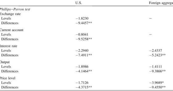
As a preliminary step, the data series are tested for unit roots.Table 1shows the results. The
seven series appear to be nonstationary in levels but stationary in first differences. This moti-vates the decision to fit the model to data in first differences. This is a common practice in the
structural VAR studies to which we wish to compare our empirical results.11The data will also
be demeaned and transformed into country differences, home minus the foreign counterpart. The last transformation of course does not apply to the exchange rate or current account, but it means that the last three variables in the data set will be movements in interest rate differen-tials, differences in output growth rates, and differences in inflation rates.
3.2. Econometric methods
The econometric methodology fits the linear approximation to the structural model, adapting a
maximum likelihood algorithm developed inLeeper and Sims (1994)and extended inKim (2000).
The linearized model equations, as derived in the section above and transformed and listed in the appendix, can be expressed in autoregressive form as
yt¼Ayt1þ3t
3twNð0;SÞ ð44Þ
whereyis the 18-element column vector of variables listed in the appendix.A is an 1818
matrix, where each cell is a nonlinear function of the structural parameters;3is a column
vec-tor, containing the five structural disturbances and where the remaining elements are zeros; and
Sis the covariance matrix of these disturbances.
The model system may be rewritten in terms of first differences as follows:
yt ¼Ayt1þ3t3t1 ð45Þ
where
10
The treasury bill rate was used for the U.S., U.K., Canada, and France; the money market rate was used for Italy; and the call money rate was used for Germany and Japan.
11
yt ¼ytyt1: ð46Þ
This stochastic model implies a log likelihood function:
LðPÞ ¼ 0:5 lnjUj 0:5x0U1
x ð47Þ
wherexis the vector of the five variables on which we have data, over all periods stacked into
a single vector, andUis the theoretical varianceecovariance matrix of the variables inx. The
appendix discusses the details of howUis computed as a function of the matricesAandS. But
note that each cell inAis a nonlinear function of the structural parameters from the theoretical
model. An algorithm is used to search for values of these structural parameters and for the
el-ements of the symmetric positive-definite covariance matrixS, which will maximize the
likeli-hood function. Note that taking first differences should not introduce the classic problem of ‘‘overdifferencing’’ here. The fact that differencing may introduce a moving average term is
taken into consideration in Eq.(45)and hence the computation ofUand the likelihood
func-tion, so a misspecified model is not being estimated.
A few parameters will not be estimated here, but instead are pinned down ahead of time. This is because the data set omits the relevant series for these parameters, like capital and labor, or because the data set in first differences is not very relevant for parameters pertaining to steady states. As a result, these parameters are pinned down at values common in the Real Business Cycle literature.
In particular, the capital share in production (a) is set at 0.40, the depreciation rate (d) is set at 0.10,
the labor supply elasticity (1/s3) is calibrated at unity, the steady state share of home intermediate
goods in the home final goods aggregate (q) is set at 0.80, and the discount factor (b) is set at 0.96.
Some regions of the parameter space do not imply a well-defined equilibrium within the model. These regions can be precluded by imposing boundaries on the parameters by functional Table 1
Unit root tests
U.S. Foreign aggregate
PhillipsePerron test
Exchange rate
Levels 1.8230 e
Differences 9.4457**
Current account
Levels 0.8041 e
Differences 9.5258**
Interest rate
Levels 2.2940 2.4337
Differences 7.4911** 5.2423**
Output
Levels 1.8986 1.4111
Differences 4.1464** 9.3866**
Price level
Levels 1.7126 3.9689*
Differences 4.3715** 9.4550**
transformations. For example, the variances of shocks and the intertemporal elasticity are re-stricted to be positive. The monetary policy reaction to inflation is bounded below to rule out indeterminacy. Autoregressive coefficients on shock processes are also restricted to be greater than zero and less than unity. Finally, the covariances between shocks must be restricted
so that the implied correlations lie between1 and 1.
4. Results
Table 2shows the basic results from estimating the model. Regarding fit, the table reports the likelihood value as 1797.6, compared to 1823.8 for a standard unidentified vector autor-egression (VAR) of the five variables in the data set. A likelihood ratio test cannot be used to
compare the two, since the structural model is not nested in the VAR.12 However, a
compar-ison can be made in terms of the Schwarz criterion, which penalizes the VAR for the fact it has 40 free parameters compared to the 24 of the structural model. By this comparison, the structural model performs better. The fit of the model can also be evaluated in terms of how well it can forecast the variables one period ahead. The table reports root mean squared errors, indicating that the structural model has larger forecast error for all five variables. It is interesting to note that the model comes closest for the exchange rate and the current account.
Perhaps a more fair comparison, given the VAR’s extra parameters, is a random walk model.
One may recall the classic result ofMeese and Rogoff (1983)that no macro model was able to
beat a random walk in forecasting the exchange rate out of sample.Table 2shows that the
struc-tural model here does beat a random walk in in-sample predictions for the exchange rate, as well as for the current account and the interest rate. Note that the predictions generated by this methodology are in sample, and hence are not directly comparable to those of Meese
and Rogoff.13
The model also does quite well in terms of fitting unconditional moments, which is the typ-ical measure of fit used in real business cycle exercises. This is a bit unfair here, given that the maximum likelihood estimation is trying to fit a set of hundreds of moments, not just a handful of arbitrary moments that researchers have in the past chosen to focus upon. Nevertheless, for the data as transformed here (in logged differences and demeaned), the variance of the exchange rate is 0.00290 in the data and 0.00293 in the model, the variance of the current
account is 1.44105in the data and 1.51105in the model, and the covariance between
the exchange rate and the current account is 6.52106in the data and 6.19106in the
model.
The parameter estimates generally are reasonable and statistically significant. The elasticity
of intertemporal substitution (1/s1) is near unity. The interest elasticity of money demand
im-plies an income elasticity of money demand (s1/s2) which is a bit high, around 4. The
invest-ment adjustinvest-ment cost (jI) is high but not implausible, implying that if investment rises 1%
above steady state, about 1.1% of this investment goes toward paying the adjustment cost.
12Given the unobserved variables in the structural model, it cannot be written as a first-order VAR in just the five ob-served variables. SeeBergin (2003)for details.
13
The adjustment cost on prices (jP) is quite reasonable, indicating that after a money supply
shock the half-life of price-level adjustments is about five quarters.
Some of the parameters estimated here deal directly with points of controversy in the the-oretical New Open Economy Macro literature. One such controversy regards the functional Table 2
Estimation results
Measures of fit Log likelihood value
Model 1797.55
Standard VAR 1823.78
Schwarz criterion
Model 1741.14
Standard VAR 1642.81
RMSE: structural model/standard VAR
Exchange rate 1.013
Current account 1.019
Interest rate 1.104
Output 1.092
Price level 1.171
RMSE: structural model/random walk
Exchange rate 0.984
Current account 0.986
Interest rate 0.997
Output 1.045
Price level 1.037
Parameter estimates Behavioral parameters
Consumption elasticity term s1 1.072 (0.006)
Money demand elasticity term s2 0.253 (0.003)
Investment adjustment cost jI 21.523 (0.512)
Price adjustment cost jP 31.099 (2.414)
Bond cost jB 0.00384 (0.00010)
Share of local currency pricing h 0.999 (0.000) Elasticity of substitution between home and foreign goods m 1.130 (0.062)
Monetary policy rule parameters
Response to inflation a1 0.9891 (0.0002)
Response to output a2 0.0001 (0.0000)
Response to the exchange rate a3 0.1128 (0.0138)
Shock autocorrelations
Technology 0.9671 (0.0003)
Monetary 0.9309 (0.0089)
Tastes 0.9773 (0.0014)
Home bias 0.8908 (0.0046)
UIP deviation 0.9750 (0.0034)
Correlations with UIP shock
Technology 0.123 (0.035)
Monetary 0.152 (0.029)
Tastes 0.845 (0.011)
Home bias 0.427 (0.016)
form of consumer preferences. A common practice in the literature has been to assume Cobbe Douglas preferences between home and foreign goods, implying a unitary elasticity of substi-tution. This form has convenient risk-sharing properties in many NOEM models, which facil-itate analytical solution. This assumption stands in contrast to studies based on micro-level
evidence, which have tended to suggest higher elasticities around 5 (seeHarrigan, 1993).
How-ever, there has been a recent defense of a unit elasticity for macro-level data. One might imag-ine that there is less substitutability between home goods as an aggregate and foreign goods as an aggregate, which is the concept relevant for our macro modeling, than between home and
foreign versions of an individual variety of good (seePesenti, 2002). The estimate of the
elas-ticity of substitution in the present model supports this hypothesis.Table 2reports a level ofm
quite close to unity; while it is significantly different from zero statistically, it is not signifi-cantly different from unity. This lends empirical support to the common practice which the the-oretical literature has found so convenient.
Another controversy regards the choice of currency in which prices are sticky.Betts and
De-vereux (2000)argue that assuming prices are sticky in the currency of the buyer (local currency
pricing) improves a model’s ability to explain exchange rate behavior. On the other hand,
Ob-stfeld and Rogoff (2000)argue in favor of prices sticky in the currency of the seller (producer currency pricing). As explained above, this model is set up to allow both types of price-setters
to coexist, and the share of local currency pricing firms,h, is a parameter that can be estimated
empirically.Table 2shows that the estimate of this share presses up against the upper bound of
unity.14This indicates strong support for the use of local currency pricing in NOEM models, in
as much as this provides a useful way of explaining the macroeconomic times series examined here.
Table 2also provides an estimate forjB, which characterizes the sensitivity of a country’s
interest rate premium to changes in net foreign assets. The estimated value of 0.00384 implies that when a G7 country runs a net foreign debt that is 20% of GDP (a relevant value for the U.S.), its domestic interest rate would rise by 7.68 basis points. This is very close to the
cali-brated value used inNason and Rogers (2003)based on empirical work for Canada, but
some-what lower than the value estimated from panel and cross-sectional regressions inLane and
Milesi-Ferretti (2002).15It is hoped that this estimate might prove useful as a basis for calibra-tions in future theoretical work.
Finally, the table also lists parameters in the monetary policy reaction function. Since the
estimate ofa1is close to its boundary of unity, the monetary response to inflation is close to
its lower bound of (1/ba1), imposed to ensure a unique equilibrium. This suggests that the
model might fit the data better if we permitted it to explore regions of the parameter space
that involved indeterminacy, as has been suggested byLubik and Schorfheide (2004). The
re-sponse to output (a2) is near zero, indicating little evidence of active output stabilization. The
statistically significant estimate ofa3indicates some systematic response to stabilize exchange
rates by some countries.16
14The standard error appears very small here, because the estimation algorithm estimates a functional transformation of this parameter, with a range over (N,N) rather than the range of (0,1) of the original parameter. A large section of the range over which the algorithm searches is mapped into a narrow range of the reported parameter near its upper bound of unity. The delta method thus reports small standard errors in terms of the original parameter value.
15
Lane and Milesi-Ferretti (2002) estimate a value of 0.0107 from cross-sectional regressions and a value of 0.0254 from panels.Nason and Rogers (2003)use a value of 0.0035.
16
Table 2is also informative about the nature of structural shocks. Of particular interest are the
correlations at the bottom of the table.Obstfeld and Rogoff (2002)have posited an NOEM model
in which monetary policy accounts for deviations from interest rate parity. But the estimated model here indicates that the deviations from interest rate parity we observe in the data have fairly little to do with any monetary policy innovation or with technology shocks. However, there is a high degree of negative correlation with the taste shocks defined in this model (correlation
co-efficient of0.86). This result is interesting, as the taste shock (t) directly affects marginal utility,
which is an important element in the risk premium term dropped from the UIP condition due to linearization, as discussed above. Additional interpretation of this relationship between taste shocks and interest rate parity deviations will follow below. Estimates of shock variances do not lend themselves to direct interpretation and are not shown in the table, but these will be inter-preted in the form of variance decompositions to follow shortly. The shock autocorrelations indi-cate a fairly high degree of persistence in all the shocks. Fortunately, none presses up against the boundary of unity, required to maintain stationarity of the theoretical system.
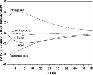
Impulse responses offer a greater sense of what these parameters imply for the dynamics of
the economy.Fig. 1 shows the impulse responses of the five data variables to a one standard
deviation shock to the monetary policy rule. As the interest rate rises, this induces an immediate
fall in output and a gradual fall in the price level.17The monetary contraction induces a
signif-icant exchange rate appreciation, in which the exchange rate overshoots. It also involves a small degree of worsening in the current account.
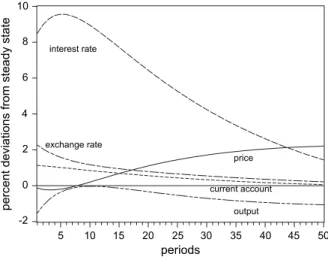
Fig. 2illustrates an interest rate parity shock in the context of this model. Such a shock per-mits the home interest rate to rise relative to the foreign rate, even though the value of the do-mestic currency is appreciating over time, as is often observed empirically. The shock may be understood as a type of portfolio shift away from home assets, such that an excess return is re-quired to make households willing to hold home bonds in equilibrium. While this shock is often used as a shorthand way of introducing exchange rate fluctuations in an NOEM model, it is
-6 -4 -2 0 2 4 6
5 10 15 20 25 30 35 40 45 50
current account interest rate
exchange rate price output
periods
percent deviations from steady state
Fig. 1. Impulse responses for a one standard deviation monetary policy shock.
17
interesting to note that this shock implies movements in a variety of variables, not just the ex-change rate. In particular, the interest rate moves substantially here, and there is also a sizeable response in the current account.
Given the apparent relationship between the interest parity shock and the taste shock,Fig. 3is
included to show the impulse response to the latter. It implies a case where the current account moves
in very much the same way as inFig. 2for an interest parity shock, but the exchange rate moves in the
opposite direction. If these two shocks indeed are highly negatively correlated, the combination of the two would imply a large change in the exchange rate, while any effect on the current account is substantially canceled out. This observation will be useful in the analysis below.
A natural question is, how important are the interest parity shocks to these results? In par-ticular, is the model able to explain the exchange rate simply because it can invoke the UIP
-2 0 2 4 6 8 10
current account interest rate
exchange rate
price
output
5 10 15 20 25 30 35 40 45 50
periods
percent deviations from steady state
Fig. 2. Impulse responses for a one standard deviation interest rate parity shock.
-5 -4 -3 -2 -1 0 1 2 3
current account
interest rate exchange rate
price
output
5 10 15 20 25 30 35 40 45 50
periods
percent deviations from steady state
shock to drive the exchange rate as needed to match the data? To address this question one can consider variance decompositions, which show what fraction of the forecast error variance for each variable is explained by each of the shocks at various time horizons. This analysis is com-plicated somewhat by the fact that UIP deviations are allowed to be correlated here with the four structural shocks. Recall that this choice was made because UIP deviations do not strictly arise from the structural model, and because we wished to gather information that might help us interpret these UIP deviations and offer guidance to future modelers. As a result, to disentangle the various contributions of these shocks, one must take steps to orthogonalize them. It might seem that a natural approach would be to re-estimate the model, requiring the shocks to be or-thogonal. However, this estimation produced a likelihood value of only 1755.737. This version
of the model may be regarded as nested in the benchmark case shown inTable 2, with the
ad-dition of four restrictions requiring the correlations between shocks to be zero. As a nested comparison, a likelihood ratio test can be used, where twice the difference of the likelihood
values follows a chi-squared distribution with four degrees of freedom. Thep-value of such
a comparison is zero, indicating we should reject the restrictions. Because the model that as-sumes orthogonal shocks is strongly rejected by the data, I will continue to utilize the model that permits them to be correlated.
As a result, we must take a stand on how to disentangle the joint contribution of the UIP and
other shocks.Table 3shows variance decompositions which orthogonalize the UIP shock by
attributing any joint contribution shared between the UIP and another shock to that other
shock.18 The table shows that the independent part of UIP shocks explains only about 1% of
exchange rate movements in this model. This suggests that the UIP shock is not being used here to drive the exchange rate and artificially boost the model fit. Instead, a bit more than half of the exchange rate movements appear to be driven by monetary policy shocks. This result
is comparable to that found in past studies.Eichenbaum and Evans (1995)found variance
de-compositions between 18% and 43% using standard VAR techniques.Rogers (1999)found
be-tween 19% and 60%.Faust and Rogers (2003)found estimates ranging from the single digits to
around 50% using a structural VAR that considered a wide range of identification assumptions.
Ahmed et al. (1993)found almost no role for monetary shocks in a structural VAR using long-run identification restrictions. In our estimation, taste shocks also have some importance, ex-plaining about 25% of exchange rate movements.
In contrast, for the current account,Table 3shows that a surprisingly large role is played by
the UIP shock. Nearly two-thirds of current account movements are attributable to these shocks, which raise an interesting possibility. These UIP shocks represent portfolio shifts in the asset market between countries, which naturally affect a country’s capital account. These shocks to the capital account then should affect the current account through the balance of payments identity. The model seems to be suggesting that attempts in the New Open Economy literature to explain current account movements in terms of optimal intertemporal saving decisions may be misplaced. Rather, the current account could be driven substantially by financial shocks af-fecting the capital account side of the balance of payments, which then forces adjustment in
saving and investment on the current account side. This conjecture should be pursued in the future in the NOEM literature.
For completeness,Table 4shows variance decompositions with the opposite method of
or-thogonalization, where comovements in the UIP shock with other shocks is awarded instead to the UIP shock. By this accounting, the role of UIP shocks in driving exchange rates goes up somewhat, but it still explains less than a quarter of exchange rate movements at its maximum. Monetary policy shocks still are the main explanation and account for about half of the forecast error variance. Given that it is the coincidence of UIP deviations with other shocks that affects the variance decomposition, one may conclude that UIP shocks have their greatest usefulness in Table 3
Variance decompositions (remove correlated components of interest parity shock)
Period Shocks
Technology Monetary policy Tastes Home basis Interest parity
Exchange rate 1 0.11 0.54 0.26 0.07 0.01
2 0.10 0.57 0.26 0.06 0.01
3 0.09 0.59 0.25 0.06 0.01
4 0.08 0.61 0.25 0.06 0.01
5 0.07 0.62 0.25 0.05 0.01
10 0.05 0.66 0.24 0.04 0.01
20 0.04 0.66 0.25 0.04 0.01
Current account 1 0.24 0.00 0.07 0.05 0.64
2 0.28 0.00 0.06 0.03 0.64
3 0.30 0.00 0.05 0.02 0.62
4 0.32 0.01 0.04 0.03 0.60
5 0.33 0.01 0.04 0.04 0.58
10 0.35 0.03 0.02 0.14 0.47
20 0.32 0.05 0.01 0.27 0.36
Interest rate 1 0.48 0.16 0.31 0.01 0.04
2 0.39 0.19 0.36 0.02 0.04
3 0.32 0.21 0.39 0.03 0.05
4 0.27 0.22 0.42 0.04 0.05
5 0.22 0.23 0.45 0.05 0.05
10 0.11 0.24 0.51 0.09 0.05
20 0.06 0.22 0.55 0.11 0.05
Output 1 0.16 0.16 0.37 0.31 0.01
2 0.22 0.12 0.41 0.24 0.01
3 0.28 0.10 0.44 0.18 0.00
4 0.32 0.08 0.46 0.14 0.00
5 0.35 0.06 0.47 0.11 0.00
10 0.44 0.03 0.49 0.05 0.00
20 0.47 0.02 0.49 0.02 0.00
Price level 1 0.50 0.29 0.13 0.07 0.00
2 0.50 0.30 0.13 0.07 0.00
3 0.51 0.30 0.13 0.07 0.00
4 0.51 0.30 0.13 0.06 0.00
5 0.51 0.30 0.13 0.06 0.00
10 0.53 0.31 0.13 0.04 0.00
explaining exchange rate movements not as an independent factor, but as a way of modifying the effect of other shocks. For example, recall from above that taste and UIP shocks are highly negatively correlated. Recall also from the discussion of impulse responses that the combina-tion of an UIP and a negative taste shock implies a large movement in the exchange rate with a net effect on the current account that is near zero. The estimated model thus suggests a channel for explaining the ‘‘relative price puzzle’’ and the ‘‘exchange rate disconnect puzzle’’ noted in
several papers (seeFlood and Rose, 1999; Duarte and Stockman, 2001; Devereux and Engel,
2002). That is, the structural model has found one way to account for the fact that volatility
of the exchange rate tends to be high relative to quantity variables like the current account, Table 4
Variance decompositions (remove correlated components of other shocks with interest parity shock)
Period Shocks
Technology Monetary policy Tastes Home basis Interest parity
Exchange rate 1 0.08 0.48 0.19 0.00 0.25
2 0.07 0.49 0.20 0.00 0.24
3 0.06 0.51 0.20 0.00 0.23
4 0.05 0.52 0.21 0.00 0.22
5 0.04 0.53 0.21 0.00 0.21
10 0.03 0.56 0.22 0.00 0.19
20 0.02 0.56 0.23 0.00 0.18
Current account 1 0.25 0.17 0.54 0.04 0.00
2 0.28 0.15 0.55 0.02 0.00
3 0.30 0.13 0.54 0.02 0.01
4 0.31 0.11 0.53 0.02 0.03
5 0.32 0.10 0.52 0.02 0.04
10 0.31 0.05 0.45 0.08 0.10
20 0.27 0.03 0.37 0.17 0.15
Interest rate 1 0.58 0.06 0.03 0.04 0.29
2 0.50 0.07 0.03 0.03 0.37
3 0.42 0.08 0.03 0.03 0.44
4 0.36 0.08 0.03 0.02 0.50
5 0.31 0.09 0.03 0.02 0.55
10 0.17 0.09 0.03 0.01 0.69
20 0.10 0.09 0.02 0.01 0.78
Output 1 0.14 0.09 0.21 0.51 0.06
2 0.19 0.07 0.19 0.44 0.11
3 0.23 0.06 0.17 0.38 0.16
4 0.27 0.05 0.16 0.33 0.20
5 0.29 0.04 0.14 0.29 0.24
10 0.35 0.02 0.10 0.19 0.34
20 0.38 0.01 0.09 0.13 0.40
Price level 1 0.41 0.20 0.03 0.00 0.36
2 0.41 0.20 0.03 0.00 0.36
3 0.41 0.21 0.03 0.00 0.35
4 0.42 0.21 0.03 0.00 0.35
5 0.42 0.21 0.03 0.00 0.34
10 0.44 0.22 0.02 0.00 0.31
where large movements in the former have little impact on the latter.19Future theoretical work may wish to pursue this suggestion, by looking for sources of interest rate parity deviations that involve shifts in marginal utilities.
5. Conclusions
This paper has advanced the New Open Economy Macroeconomic literature in an empirical direction, fitting a two-country model by maximum likelihood to data from the U.S. and an aggre-gate of the remaining G7. The model fits reasonably well, in that it is able to beat a random walk model for in-sample predictions of the exchange rate and current account, variables of key interest to open economy macroeconomists. The estimated model facilitates empirical answers to a num-ber of interesting questions raised recently in the theoretical literature. For example, it gives em-pirical support to the assumption of local currency pricing by firms, as well as to the common simplifying assumption of a unitary elasticity of substitution between home and foreign goods. It also provides an estimate for how a country interest rate premium responds to changes in net foreign debt positions, an estimate which might prove useful as a basis for calibrations of future theoretical models. In addition, the exercise indicates that deviations from interest rate parity do not seem to be closely related to monetary policy, as has been hypothesized in recent theory, but that these deviations do seem to be related to shifts in marginal utilities of consumption. Further, the model indicates that such interest rate parity shocks are not especially helpful as independent explanations for exchange rate movements observed in the data. But on the other hand, these shocks are helpful in explaining movements in the current account. It is hoped that this study may prove helpful for discriminating between alternative theoretical models currently being pro-posed, and for suggesting productive avenues for future theoretical research.
Acknowledgements
I thank the participants in the 2003 AEA meetings and the CEPR International Capital Mar-kets conference in Rome 2003 for helpful comments. I thank Ivan Tchakarov for excellent research assistance. This material is based upon work supported by the National Science Foundation under Grant No. 0109006. Any opinions, findings, and conclusions or recommen-dations expressed in this material are those of the author and do not necessarily reflect the views of the National Science Foundation.
Appendix A
A.1. List of equilibrium conditions
These equations are used in linearized form, expressed as differences between the home country variables and foreign country counterparts. The system may be written in the following
18 variables: ctct*, ltlt*, ytyt*, ptp*t, wtwt*, pFtpH*t, pHtpF*t, yHtyF*t,yFtyH*t,
zHtzH*t,itit*,ktkt*,rtrt*,BtBt*,MtMt*,st,cat,xt. Numbered below are the 18
line-arized conditions that determine these sequences. Country size isn.
Linearized home consumption Euler:
s1cttt¼s1Etðctþ1Þ Etðttþ1Þ þEt½Ptþ1 Pt ð1bÞit
together with the foreign counterpart:
s1ctt
t ¼s1Et
ctþ1Et
ttþ1þEt
Ptþ1Pt ð1bÞit
to form:
s1
ctct
tttt
¼s1Et
ctþ1ctþ1
Et
ttþ1ttþ1
þEt
Ptþ1Ptþ1
PtPt
ð1bÞitit
: ð48Þ
Money demand:
s1ctþs2pts2mttt b2
1bit¼0
combined with foreign:
s1
ctct
þs2
ptpt
s2
mtmt
tttt
b
2
1b
itit
¼0: ð49Þ
Labor supply:
1 s3
ltlt
¼wtwt
s1
ctct
ptpt
þ ð1s1Þ
tttt
: ð50Þ
Production function:
ztzt
¼atat
þakt1kt1
þ ð1aÞltlt
: ð51Þ
The linearized price setting rule for domestic sales by local currency pricing (lcp) firms is:
½vðyHtðlcpÞ yHtÞ þmct ½1þnpHtþ ½n ð1þbÞvjPpHtðlcpÞ þ ½vjPpHt1ðlcpÞ þ ½bvjPEtpHtþ1ðlcpÞ ¼0
where
mct¼ptþrtatþ ð1aÞkt1 ð1aÞlt:
The linearized price setting rule for domestic sales is the same for producer currency pricing (pcp) firms:
Given that all local currency pricing firms set the same price as each other, and all producer currency pricing firms as each other, we may write the linearized form of the home domestic goods price index as:
pHt¼hpHtðlcpÞ þ ð1hÞpHtðpcpÞ:
Substituting in the price-setting equations above, we find the overall price level of home goods sold at home:
mct ½1þ ð1þbÞvjPpHtþ ½vjPpHt1þ ½bvjPEtpHtþ1¼0:
The foreign counterpart is
mct ½1þ ð1þbÞvjPpFtþ ½vjPpFt1þ ½bvjPEtpFtþ1¼0
where
mct ¼pt þrt1atþ ð1aÞkt1 ð1aÞlt:
Similarly, the linearized price setting rule when home local currency pricing firms
(i¼0,.,h) export is:
½nyHtðlcpÞ yHtþmct ½1þnpHtþ ½n ð1þbÞvjPpHtðlcpÞ þ ½vjPpHt1ðlcpÞ þ ½bvjPEtpHtþ1ðlcpÞ st¼0:
And for producer currency pricing firms, this is:
vyHtðpcpÞ yHtþmct ½1þnpHtþ ½n ð1þbÞvjPpHtðpcpÞ þ ½vjPpHt1ðpcpÞ þ ½bvjPEtpHtþ1ðpcpÞ ½1þvst¼0:
Since the linearized form of the home export price index implies:
pHt¼hpHtðlcpÞ þ ð1hÞpHtðpcpÞ ð1hÞst;
we can substitute in the pricing equations to write an equation for this export price index as:
mct ½1þ ð1þbÞvjPpHtþ ½vjPpHt1þ ½bvjPEtpHtþ1 ½ð1hÞð1þbÞnjPþ1st
þ ð1hÞnjPst1þ ð1hÞbnjPEt½stþ1 ¼0:
The counterpart for foreign country exports to the home country is:
mct ½1þ ð1þbÞvjPpFtþ ½vjPpFt1þ ½bvjPEtpFtþ1þ ½ð1hÞð1þnÞ þ1st
ð1hÞnjPst1 ð1hÞbnjPEt½stþ1 ¼0:
Then combine these four pricing equations to get:
mctmct
½1þ ð1þbÞvjPpHtpFt
þ ½vjPpHt1pFt1
þ ½bvjPEt
pHtþ1pFtþ1
and
mctmct
½1þ ð1þbÞvjPpFtpHt
þ ½vjPpFt1pHt1
þ ½bvjPEtðpFtþ1Þ Et
pHtþ1
2½ð1hÞð1þbÞnjPþ1st
þ2ð1hÞnjPst1þ2ð1hÞbnjPEt½stþ1 ¼0: ð53Þ
Ratio of price indexes:
pt¼qpHtþ ð1qÞpFtþqlogð1qtÞ
pt ¼1qpHtþqpFtþqlog1qt
so
ptpt
¼1qpFtpHt
þqpHtpFt
: ð54Þ
Demands are
yHt¼ytþmptmpHtqt
yFt¼ytþmptmpFt
q
1q
qt
yFt¼ytþmpt mpFtþqt
yHt¼yt þmptmpHt
q
1q
qt
so
yHtyFt
¼ytyt
þmptpt
mpHtpFt
þqtqt
ð55Þ
yFtyHt
¼ytyt
þmptpt
mpFtpHt
q
1q
qtqt
: ð56Þ
Capital accumulation:
ð1þbÞjIktbjIEtktþ1jIkt1 ð1bð1dÞÞrtþ1þbd dts1ctþs1Etctþ1 þ ð1s1Þtt ð1s1ÞEt½ttþ1 ¼0
combined with foreign:
ð1þbÞjIktkt
bjIEt
ktþ1ktþ1
jIkt1kt1
ð1bð1dÞÞrtrt
þbddtdt
s1
ctct
þs1Et
ctþ1ctþ1
þ ð1s1Þ
tttt
ð1s1ÞEt
ttþ1ttþ1
¼0:
Capital stock transition function:
ditit
¼ktkt
ð1dÞkt1kt1
ð58Þ
Capital-labor trade-off:
ptpt
þrtrt
þkt1kt1
¼wtwt
þltlt
: ð59Þ
Define final goods demand:20
ytyt
¼C
Y
ctct
þI
Y
itit
ð60Þ
Goods market clearing conditions are
qyHtþ ð1qÞyHt¼zt
ð1qÞyFtþqyFt¼z
t; so combining:
qyHtyFt
ð1qÞyFtyHt
¼ztzt
: ð61Þ
Define trade balance: (takingXas a share of GDP,Z)
1
1q
xt¼st
pFtpHt
yFtyHt
: ð62Þ
Define current account (as share of GDP):
cat¼
btsbt
bt1sbt1
: ð63Þ
Rewrite the balance of payments condition (deviations as shares of GDP):
xtþ 1 b
bt1sbt1
btsbt
¼0: ð64Þ
Linearize the interest rate parity condition, as discussed above:
itit ¼ 1
1bðEtstþ1stÞ jBðbtsb
tÞ þxt: ð65Þ
A.2. Econometric methods
The contemporaneous covariances matrix,Ryð0Þ, can be written as follows:
Ryð0ÞhEyty0t ¼Sþ XN
i¼0
BDiðDIÞB1SBDiðDIÞB10 ð66Þ
20
whereDis the diagonal matrix of eigenvalues andBthe matrix of eigen vectors ofA1:Ryð0Þ can then be computed:
Ryð0Þ ¼SþB½KB0 ð67Þ
where the typical element (i,j) ofKis
Kij¼
ð1diÞ
1dj
Mij
1didj
for dis1 ordjs1
0 for di¼1 anddj¼1
ð68Þ
and where
M¼B1SB10: ð69Þ
OnceRyð0Þis computed, the covariances across one lagRyð1Þmay be found:
Ryð1Þ ¼Eytyt0¼ARyð0Þ S ð70Þ
and over lags greater than one:
RyðkÞ ¼Eyty0t
k
¼Ak1Ryð1Þ for k>1: ð71Þ
The full covariance matrix,U, then can be constructed by assembling the blocks for various
lags. In particular, the only parts of each covariance block used are those relating to the
partic-ular data series to be fit, wherextis the relevant portion ofy*(in percent deviations from the
previous period). Further, to reduce numerical problems associated with rounding error, lags of only up to 15 periods are currently used, with covariances assumed to be zero over lags greater than 15 periods.
References
Ahmed, S., Ickes, B., Wang, P., Yoo, B.S., 1993. International business cycles. American Economic Review 83, 335e
359.
Bergin, P., 2003. Putting the new open economy macroeconomics to a test. Journal of International Economics 60, 3e34.
Bergin, P., Sheffrin, S., 2000. Interest rates, exchange rates, and present value models of the current account. The Eco-nomic Journal 110, 535e558.
Betts, C., Devereux, M.B., 2000. Exchange rate dynamics in a model of pricing-to-market. Journal of International Eco-nomics 50, 215e244.
Devereux, M.B., Engel, C., 2002. Exchange rate pass-through, exchange rate volatility, and exchange rate disconnect. Journal of Monetary Economics 49, 913e940.
Duarte, M., Stockman, A., 2001. Rational speculation and exchange rates. NBER Working Paper 8362.
Eichenbaum, M., Evans, C.L., 1995. Some empirical evidence on the effects of shocks to monetary policy on exchange rates. Quarterly Journal of Economics 110, 975e1009.
Faust, J., Rogers, J.H., 2003. Monetary policy’s role in exchange rate behavior. Journal of Monetary Economics 50, 1403e1424.
Flood, R., Rose, A., 1999. Understanding exchange rate volatility without the contrivance of macroeconomics. Eco-nomic Journal 109, 660e672.
Ghosh, A.R., 1995. International capital mobility among the major industrialised countries: too little or too much? Eco-nomic Journal 105, 107e128.
Harrigan, J., 1993. OECD imports and trade barriers in 1983. Journal of International Economics 35, 91e111.
Ireland, P., 1997. A small, structural, quarterly model for monetary policy evaluation. Carnegie-Rochester Conference Series on Public Policy 47, 83e108.
Ireland, P., 2001. Sticky-price models of the business cycle: specification and stability. Journal of Monetary Economics 47, 3e18.
Jeanne, O., Rose, A., 2002. Noise trading and exchange rate regimes. Quarterly Journal of Economics 117, 537e569.
Kim, J., 2000. Constructing and estimating a realistic optimizing model of monetary policy. Journal of Monetary Eco-nomics 45, 329e359.
Kollmann, R., 2001. Macroeconomic effects of nominal exchange rates regimes: new insights into the role of price dy-namics. University of Bonn mimeo.
Kollmann, R., 2002. Monetary policy rules in the open economy: effects on welfare and business cycles. Journal of Monetary Economics 49, 989e1015.
Lane, P.R., Milesi-Ferretti, G.M., 2002. Long-term capital movements. NBER Macroeconomics Annual, 73e116.
Leeper, E., Sims, C., 1994. Toward a modern macroeconomic model usable for policy analysis. NBER Macroeconomic Annual, 81e118.
Lewis, K., 1995. Puzzles in International Financial Markets. In: Grossman, G., Rogoff, K. (Eds.), Handbook of Inter-national Economics, vol. III. Elsevier, Amsterdam, pp. 1913e1971.
Lubik, T., Schorfheide, F., 2004. Testing for indeterminacy: an application to U.S. monetary policy. American Economic Review 94, 190e217.
Mark, N., Wu, Y., 1998. Rethinking deviations from uncovered interest parity: the role of covariance risk and noise. Economic Journal 108, 1686e1706.
McCallum, B., Nelson, E., 1999. Nominal income targeting in an open-economy optimizing model. Journal of Mone-tary Economics 43, 553e578.
McCallum, B., Nelson, E., 2000. Monetary policy for an open economy: an alternative framework with optimizing agents and sticky prices. Oxford Review of Economic Policy 16, 74e91.
Meese, R.A., Rogoff, K., 1983. Empirical exchange rate models of the seventies: do they fit out of sample? Journal of International Economics 14, 3e24.
Nason, J.M., Rogers, J.H., 2003. The present-value model of the current account has been rejected: roundup the usual suspects. Federal Reserve Bank of Atlanta Working Paper 2003-7a.
Obstfeld, M., Rogoff, K., 2000. New directions for stochastic open economy models. Journal of International Econom-ics 50, 117e153.
Obstfeld, M., Rogoff, K., 2002. Risk and exchange rates. In: Helpman, E., Sadka, E. (Eds.), Contemporary Economic Policy: Essays in Honor of Assaf Razin. Cambridge University Press, Cambridge.
Pesenti, P., 2002. International monetary policy cooperation and financial market integration, discussant comments at European Central Bank International Research Forum on Monetary Policy, Frankfurt, July.
Rogers, J., 1999. Monetary shocks and real exchange rates. Journal of International Economics 49, 269e288.
Schmitt-Grohe, S., Uribe, M., 2003. Closing small open economy models. Journal of International Economics 61, 163e
185.
Sheffrin, S., Woo, W.T., 1990. Present value tests of an intertemporal model of the current account. Journal of Interna-tional Economics 29, 237e253.