PONTIFICIA UNIVERSIDAD CATÓLICA DEL PERÚ
GRADUATE SCHOOLThe AD detector array: a new tool for studying
diffractive physics at the ALICE experiment
Thesis submitted to obtain the degree of Master of Science in Physics:
Ernesto Calvo Villar
ADVISOR: Dr. Alberto Gago Medina
diffractive physics at the ALICE experiment
Ernesto Calvo Villar
Submitted to obtain the degree of Master of Science in Physics
2015
Abstract
We present a new detector array proposal for the ALICE experiment at LHC. This new subdetector is composed of four stations of scintillator pads and its main goal is to extend our current rapidity coverage. Therefore, we would have more sensitivity to tag the rapidity gaps related to the diffractive processes.
Acknowledgments
I would like to thank my advisor, Dr. Alberto Gago, for his encouragement and patience during the entire period of this work. To Rodrigo Helaconde for useful help with Pythia6 and Phojet generation. Also, Joel Jones and Eric Endress, for useful suggestions about this work.
To Jean-Pierre Revol, Martin Poghosyan and all the members of the AD group, for the great experience of developing a new detector for the ALICE experiment at the LHC.
This project would have been impossible without the computational power provided by Legion, a grid-like supercomputer facility developed by the ‘Direc-ción de Informática Académica’ (DIA). Special thanks are due to Genghis Rios and Oscar Díaz for developing Legion in the first place, and for their great and continuous support.
To my friends, Jose, Claudia, Giulliana, for the great adventures we have been through. To Carmen, for always having a kind advice when I needed one. And Darling, for bringing a smile to my face.
Finally, I would like to thanks my parents, Alfredo and Isabel, for all the sacrifices they made for me. And to my brother and sister, who somehow forgave me for being a physicist and an older brother.
Contents
Abstract ii
Acknowledgments iii
1 Introduction 1
1.1 The ALICE experiment . . . 1
1.1.1 Solenoid Magnet . . . 1
1.1.2 Central Tracking Detectors . . . 2
1.1.3 Forward Detectors . . . 7
1.1.4 The Central Trigger Processor (CTP) . . . 9
1.2 The ALICE Physics Program and observables . . . 10
1.2.1 Latest Results from ALICE . . . 11
1.2.2 Chiral Magnetic Effect in QGP . . . 11
1.2.3 Particle yields. . . 12
1.2.4 Ultra-Peripheral Collisions. . . 13
1.2.5 Flow . . . 14
2 Physics of High Energy Diffraction 17 2.1 History of Regge Theory . . . 17
2.2 The Pomeron in QCD . . . 19
2.3 Diffraction. . . 20
2.4 Kinematics of diffraction . . . 21
2.4.1 Important physical quantities . . . 21
2.4.2 Diffractive scattering and rapidity gaps . . . 23
3 The AD detector system 27 3.1 Introduction. . . 27
3.2 AD detector system . . . 30
3.3 The Geometry of the detectors . . . 31
3.3.1 ADC1 . . . 31
3.3.2 ADA1 . . . 32
3.3.3 ADA2 and ADC2. . . 33
3.3.4 Performance . . . 34
3.4 Effects of back scattering . . . 42
4 Analysis and Results 45
4.1 Trigger Definitions . . . 45
4.1.1 Minimum Bias triggers. . . 45
4.1.2 ad hoc proposal for diffractive triggers . . . 46
4.1.3 1-arm-L(R)/2-arm triggers . . . 47
4.1.4 Using the AD stations with 1-arm-L(R)/2-arm selections 49 4.1.5 Online versus Offline selection. . . 49
4.2 Trigger efficiency vs diffracted mass. . . 50
4.3 efficiency of MB triggers vs. multiplicity . . . 54
4.4 MB efficiency diffractive triggers . . . 59
4.5 SD cross section uncertainty . . . 64
List of Figures
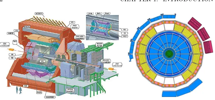
1.1 The ALICE experiment at CERN. Left: 3D view showing the diferent subdetectors and the L3 solenoid magnet (in red). Right: Cross section showing installed detectors as of 2012. . . 2 1.2 The Time Projection Chamber of ALICE. Left: Schematic view
(from [6]). Right: Tracks reconstructed by TPC in a Pb-Pb event. 3 1.3 The Inner Tracking System of ALICE. . . 4 1.4 The Transition Radiation Detector in ALICE. Left: Schematic
view. Right: Principle of operation. Adapted from [7] . . . 5 1.5 The VZERO detectors in ALICE. Left: Schematic view. Right:
Rejection of beam-gas background based on timing signals. Adapted from [1] . . . 8 1.6 Chiral Magnetic Effect (CME) in ALICE. Left: Illustration of the
charge separation with respect to the reaction plane induce by the magnetic field created by the heavy-ions. Right: Measurement of charge separation with respect to the reaction plane from the ALICE experiment [25] . . . 11 1.7 Ratios of particle yields measured by the ALICE collaboration
in lead lead collisions (right) and preliminary thermal fits to this data. Extracted from [24] . . . 12 1.8 Interaction volume in a Lead-Lead collision. From [20] . . . 15 1.9 Elliptic flow as seen by ALICE. From [21] . . . 15
2.1 Left: Leading Regge trajectories. Right: Total cross section for proton-proton (dashed line) and proton-antiproton (solid line). . 18 2.2 Left: Photon-like pomeron before QCD. Right: Pomeron as a
two gluon exchange. . . 19 2.3 The BFKL pomeron as a gluon ladder . . . 20 2.4 Scattering process in the center of mass system . . . 22 2.5 Rapidity gap in the single diffractive process 1 + 2→3 +X . . . 25
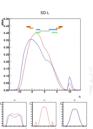
3.1 Pseudorapidity distribution of primary charged particles for dif-ferent inelastic processes according to Pythia6 (blue) and Pho-jet (red). Top: SD-L. Bottom left: Double diffractive. Bottom center: central diffraction. Bottom right: non-diffractive. The colored boxes show the pseudorapidity coverage of SPD (gray), VZERO (green), FMD (light blue), ADC and ADA (yellow), and ADC2 and ADA2 (orange) . . . 29
3.2 Diffractive mass distribution for SD-L events at √s= 7.0 (left)
and√s= 14.0TeV (right) according to Pythia6 (blue) and
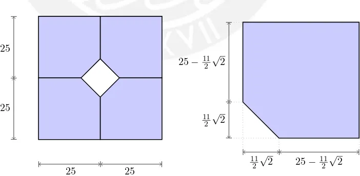
Pho-jet (red). . . 30 3.3 Left: Schematic view of the ADC1 detector. Right: detail of one
sector. All lengths are in units of centimeters. . . 32 3.4 Left: Schematic view of the ADA1 detector. Right: detail of one
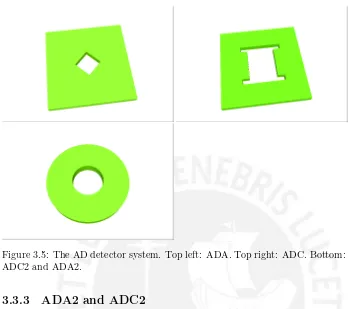
sector. . . 32 3.5 The AD detector system. Top left: ADA. Top right: ADC.
Bot-tom: ADC2 and ADA2. . . 33 3.6 Schematic view of the two configurations for the circular AD
stations. Left: geometry at z = ±55 meters. Right: at z =
±22.5meters. All lengths are in units of centimeters.. . . 34
3.7 Average charged-hit density per event per squared centimeter on the first the AD stations at an energy of√s= 7TeV. The top
plots shows the ADC atz =−1950 cm for SD-L (top left) and
SD-R (top right) diffractive events. The middle if for the ADA station (placed atz= 1700cm) for SD-L (middle left) and SD-R
(middle right). The bottom plot is for the ADC2 station (placed at z = −2250 cm) for SD-L (bottom left) and SD-R (bottom
right) . . . 35 3.8 Projection on the Z-Y plane of the origin of secondary tracks
hiting the AD stations (√s= 7TeV). From top to bottom: ADC
(z=−1950 cm), ADC2 (z =−2250 cm), ADA (z = 1700cm),
ADA2 (z=−2250cm). All the axes units are in cm. . . 37
3.9 The points (x, y) = (ηdet, ηpri)show the correlation between the
pseudorapidity of the point of impact of a charged secondary track in the AD detector and the pseudorapidity of the primary track from which the secondary originates. Top left: ADC. Top right: ADA (z = 17.0 m). Bottom left: ADC2 (z = 22.5 m).
Bottom right ADA2 (z=−22.5m). . . 38
3.10 Comparison of efficiencies of AD stations for single diffractive processes of type SD-R (left) and SD-L (right) at √s= 7(light
blue) and √s = 14 TeV (pale yellow). Top left: ADA at z = 17 m, top right: ADC at z =−19.5 m, bottom left: ADA2 at
z= 22.5 m, bottom left: ADC2 atz=−22.5m. . . 40
3.11 Pseudorapidity coverage of detectors used for diffractive triggers. In gray SPD, FMD and VZERO. In yellow proposed ADC (z=
−1950 cm)and ADA (z= 1700cm). In Orange proposed ADC2
(z=−2500cm) and ADA2 (z= +2500cm). . . 41
3.12 Results Pb-Pb . . . 43
LIST OF FIGURES ix
4.2 Comparison of the selection efficiency as function of diffracted mass for single diffractive events at√s= 7 TeV (top) and√s= 14 TeV (bottom). Left: efficiency of 1-arm-L in selecting
SD-L events. Right: efficiency of 1-arm-R in selecting SD-R events. Red boxes shows the current situation using only standard ALICE detectors (VZERO, SPD, FMD). Violet boxes uses in addition two AD counter stations (ADA and ADC). The green curve is us-ing standard ALICE and all the four AD counter stations (ADA, ADC, ADA2, ADC2). The boxes show the systematic uncertain-ties estimated from the differences between Pythia6 and Phojet. 51
4.3 Pseudorapidity of particles versus diffracted mass of the par-ent system for single diffractive evpar-ents of type SD-L (left) and SD-R (right) according to Pythia6 for an energy of7.0 TeV. The
horizontal lines show the η coverage for: SPD+VZERO+FMD
(grey), plus two (yellow) and four (orange) AD stations. For SD-L (SD-R) the patch atη ∼10 (η ∼ −10) is due to the
non-diffracted proton. . . 52
4.4 Comparison of the selection efficiency ofad hoctriggers as func-tion of diffracted mass for single diffractive events at√s= 7TeV
(top) and√s= 14 TeV (bottom). Left: efficiency of SD-L
trig-ger in selecting SD-L events. Right: efficiency of SD-R trigtrig-ger in selecting SD-R events. light blue boxes shows the current situation using only standard ALICE detectors (VZERO, SPD, FMD). Violet boxes uses in addition two AD counter stations (ADA and ADC). The green curve is using standard ALICE and all the four AD counter stations (ADA, ADC, ADA2, ADC2). The boxes show the systematic uncertainties estimated from the differences between Pythia6 and Phojet. . . 53
4.5 Efficiency in selecting diffractive events as function of multiplicity for MB-OR(0,1,2) triggers at √s = 7 TeV according to Pythia6
(blue) and Phojet (Red). Top left: SD-L. Top right: SD-R. Bottom left: double-diffraction. Bottom right: central diffrac-tion. The solid lines depict the current situation (MB-OR0).
The dashed and dotted lines shows the situation when we add two (MB-OR1) and four (MB-OR2) AD stations to the definition
of MB-OR. . . 57
4.6 Efficiency in selecting diffractive events as function of multiplicity for MB-OR(0,1,2) triggers at√s = 14TeV according to Pythia6
(blue) and Phojet (Red). Top left: SD-L. Top right: SD-R. Bottom left: double-diffraction. Bottom right: central diffrac-tion. The solid lines depict the current situation (MB-OR0).
The dashed and dotted lines shows the situation when we add two (MB-OR1) and four (MB-OR2) AD stations to the definition
List of Tables
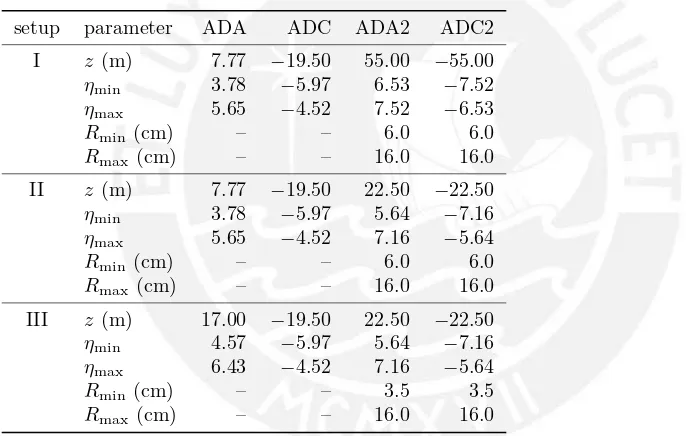
3.1 The different configurations of the AD stations simulated in this work . . . 31 3.2 Efficiency of AD stations at √sof 7and14for single diffractive
events where the diffracted mass is in the direction of the detector (SD-L for ADC and ADC2, SD-R for ADA and ADA2). For the rows labeled Pythia6 and Phojet we display the statistical error (σE). Then the average of these values is calculated and the statistical error estimated from the difference of Pythia6 and Phojet (the statistical error is ignored since it is negligible) . . . 41
4.1 Efficiency of minimum biastrigger in selecting different types of pure events using Pythia6 and Phojet at √s = 7. Note that
Pythia6 does not implement central diffraction (CD).. . . 55 4.2 Efficiency of minimum biastrigger in selecting different types of
pure events using Pythia6 and Phojet at√s= 14TeV. Note that
Pythia6 does not implement central diffraction (CD).. . . 55 4.3 Total Efficiency of MB-ORi triggers in selecting minimum bias
events at√s= 7TeV and√s= 14TeV. The error displayed show
the systematic uncertainty estimated using Pythia6 and Phojet. 55 4.4 Composition of a sample of minimum bias events according to
Pythia6 and Phojet. Note that Pythia6 does not implement cen-tral diffraction (CD). . . 60 4.5 Trigger efficiencies and purity of selected sample for √s= 7TeV
for ad hoc triggers. The values are the average of Pythia6 and Phojet. The errors displayed represent the systematic uncertainty estimated from the difference between Pythia6 and Phojet (ex-cept for central diffraction since Pythia6 does not implement it). The sub-indexes are: 0 =no AD station, 1 = two stations and 2 =four stations . . . 62
4.6 Trigger efficiencies and purity of selected sample for√s= 14TeV
for ad hoc triggers. The values are the average of Pythia6 and Phojet. The errors displayed represent the systematic uncertainty estimated from the difference between Pythia6 and Phojet (ex-cept for central diffraction since Pythia6 does not implement it). The sub-indexes are: 0 =no AD station, 1 = two stations and 2 =four stations . . . 62
4.7 Trigger efficiencies and purity of selected sample for √s= 7TeV
for 1-arm-L(R)/2-arm triggers. The values shown are the average of Pythia6 and Phojet. The errors displayed represent the system-atic uncertainty estimated from the difference between Pythia6 and Phojet. The sub-indexes are: 0 = no AD station, 1 =two
stations and2 =four stations . . . 63
4.8 Trigger efficiencies and purity of selected sample for√s= 14TeV
for 1-arm-L(R)/2-arm triggers. The values shown are the average of Pythia6 and Phojet. The errors displayed represent the system-atic uncertainty estimated from the difference between Pythia6 and Phojet. The sub-indexes are: 0 = no AD station, 1 =two
stations and2 =four stations . . . 64
Chapter 1
Introduction
1.1 The ALICE experiment
A Large Ion Collider Experiment (ALICE) is one of the seven experiments of
the Large Hadron Collider (LHC) which is located in the Franco-Swiss border and run by theEuropean Organization for Nuclear Research(CERN). Its main physics goal is the study and characterization of a new state of matter known as
quark-gluon plasma(QGP) created in high energy heavy-ion collisions. Quarks
in normal conditions are inextricably locked into the hadrons they belong, but become deconfined in this new state, forming a high density, low viscosity fluid in which they are almost free to move, and where there are no more hadronic boundaries.
To this end, ALICE participates in dedicated lead-lead runs at the LHC at a center of mass energy (CMS) per nucleon of√SN N = 2.76TeV for the study
of key QGP Observables. ALICE also collects data from proton-proton runs at an CMS energy of√S= 7TeV in order to disentangle true QGP behavior from
what could be a simple consequence of the scaling in the number of participant nucleons.
In addition to this, special p+Pb runs were performed at the end of 2012 and beginning of 2013 from which ALICE certainly profited as this allowed to confirm that observations made in Pb+Pb collisions originate from the presence of QGP.
ALICE is unique among other experiments at the LHC due to its excellent particle identification capabilities, low transverse momentumpT threshold, and
their coverage in eight units of pseudorapidity. In the following sections we describe briefly the main sub system of ALICE.
1.1.1 Solenoid Magnet
Most of the ALICE experiment detectors are surrounded by a big solenoid pro-ducing a magnetic field of0.5 Tesla in the beam (orz) direction. The purpose
of this magnetic field is to help the detectors in the central region of ALICE to identify the charged particles by measuring the bending of their path caused by the Lorentz force.
Figure 1.1: The ALICE experiment at CERN. Left: 3D view showing the diferent subdetectors and the L3 solenoid magnet (in red). Right: Cross section showing installed detectors as of 2012.
1.1.2 Central Tracking Detectors
Time Projection Chamber (TPC)The TPC is the main tracking device of ALICE. It is able to reconstruct the three-dimensional path of the charged particles that traverse its volume and allows for charged particle momentum measurements (through the bending of the track in the ALICE solenoid magnetic field), charged particle identification (viadE/dxmeasurements), track reconstruction and vertex determination.
The TPC consists of a cylindrical chamber with its symmetry axis oriented parallel to the beam pipe (fig.1.2) and filled with a Ne/CO2/N2(85.7%/9.5%/4.8%)
gas mixture at atmospheric pressure. Inside the TPC, a thin foil electrode lo-cated at its center divides the TPC in two halves. A difference of potential is applied between this electrode and the end caps creating an electric field parallel to the z axis. In addition to the electric field, the external solenoid magnet of
ALICE creates a magnetic field of0.5 Tesla parallel to the TPC axis.
The principle of operation of the TPC is the following [13]: When a charged particle traverse the volume of the TPC, it ionizes the gas molecules of the medium releasing a trail of electrons and ions. The electrons are then pulled towards the end caps of the TPC due to the electric field (400V/cm) previously
mentioned, leaving a projection in the XY plane of the tracks. Under this
combination of field strength, gas mixture and pressure, the maximum drift time of the electrons is of 90µs. During this time the traveling image of the track
is broadened by the transverse diffusion of electrons during the drift. Normally this would affect the resolution in the determination of the track. However, in the TPC, the Lorentz force on the drifting electrons (generated by theXY
component of their velocity and the axial magnetic field) reduce this effect by forcing the electrons to move in helical paths toward the end caps.
1.1. THE ALICE EXPERIMENT 3
strong enough as to produce secondary ionization, i.e, to deliver the required kinetic energy to electrons so that they are able to strip some electrons in their next collision with a gas molecule. This process is repeated over and over generating an amplification by avalanche of the signal. In a cathode readout MPWC the cathode planes are also made of parallel wires oriented perpendicular to the direction of the anode wires allowing an increase in the position resolution. After this anXY projection of the ionizing track is created in the end caps
and thez coordinate is inferred from the arrival time of the electrons. With all
this information the TPC is able to make a full 3D reconstruction of the track. If a the track leaves clusters in ITS, TRD, TOF and TPC it is called a track with full radial length. For these tracks the information from different detectors can be combined to obtain a more accurate particle identification on momentum resolution. The pseudorapidity coverage of TPC in this case is|η|<0.9
If we only require the tracks to hit anywhere in the TPC then the pseudo-rapidity coverage is |η|<1.5(reduced track length). The ALICE TPC is able
[image:15.595.109.438.320.490.2]to observe tracks from lowpT of0.1 GeV/c up to100GeV/c.
Figure 1.2: The Time Projection Chamber of ALICE. Left: Schematic view (from [6]). Right: Tracks reconstructed by TPC in a Pb-Pb event.
Inner Tracking System (ITS)
The ITS consist of six layers of silicon detectors (fig.1.3), located at4, 7, 15, 24,39and44cm from the beam line. Their mission is the determination of the
primary vertex and the tracking and identification of particle with momentum below100 MeV.
In semiconductor detectors [13] a charged particle traversing a volume of this material will create electron-hole pairs by exciting electrons from the valence band to the conduction band leaving behind a hole in the valence band. The electrons will dissipate their remaining energy by producing more electron-hole pairs (excitons) and by exciting lattice oscillations (phonons). This leaves a zone around the path traversed by the particle with a high concentrations of electrons and holes (1015 to1017 per cm3). In order to get a detectable signal
This can be achieved by using p−n junctions with a reverse bias voltage.
A p−n junction is the frontier between a zone in the semiconductor material
doped with electron acceptor impurities and another doped with electron donor impurities. When a reverse bias electric field is applied to thep–n junction, a
rearrangement of the charge carriers and the valence and conduction bands near the border creates the adequate condition for the collection of charges left by the charged track.
Silicon Pixel Detector (SPD) It makes up the first 2 layers of the ITS. The SPD is made up of 240 ladders, each one with a sensitive area of12.8mm
(rφ) × 69.6mm (z). The ladder is a silicon pixel sensor matrix consisting of
256×160 cells, each cell measuring 50µm in the rφdirection and 425 µm in
thezdirection. Two ladders are mounted along thez axis to form a half-stave.
Then, the half-staves are mounted in carbon-fibre supports called sectors. Each sector supports 6 half-staves, two for the inner layer and four for the outer layer. Ten sectors are mounted together around the beam pipe to fully cover the azimuthal angle. So we have 80 ladders for the inner layer of SPD and 160 for the outer layer. This detector is capable of providing fast signal triggers.
Silicon Drift Detectors (SDD) The Silicon Drift Detectors equip the two intermediate layers of the ITS, where the charged particle density is expected to reach up to 7 particles per cm2. They have a very good multi-track capability
and providedE/dx measurements needed for the ITS particle identification
Silicon Strip Detectors (SSD) The outer layers of the ITS are crucial for the connection of tracks from the TPC to the ITS. They also providedE/dx
[image:16.595.213.399.523.687.2]in-formation to assist identification of low-momentum particles. Both outer layers consist of double-sided Silicon Strip Detectors (SSD), mounted on carbon-fibre support structures identical to the ones used in SDD.
1.1. THE ALICE EXPERIMENT 5
Transition-Radiation Detector (TRD)
The TRD detector (fig. 1.4) surrounds the TPC in the pseudorapidity range |η| ≤ 0.9. The main goal of the TRD is to provide electron identification in
the central barrel for particles with momentum greater than 1 GeV/c, where
the pion rejection capability through energy loss measurement in the TPC is no longer sufficient. The principle of operation of the TRD is the following:
Figure 1.4: The Transition Radiation Detector in ALICE. Left: Schematic view. Right: Principle of operation. Adapted from [7]
When a highly relativistic (γ > 103) charged particle crosses the boundary
between two medium of different refraction index (n), a forward cone of soft
X-ray photons is produced with a characteristic peak near to the polar angle given by ϕ≈1/γ. This is called transition-radiation (TR) and its intensity is
proportional toγ= 1/√
1−β2for a single boundary crossing.
This production can be understood in a qualitative way if we imagine that the particle, while approaching the boundary to the denser medium, forms to-gether with its image, an electric dipole. The field strength of this dipole varies as the particle gets closer to the boundary and vanishes upon entering to the denser medium. The sudden variation in time of the dipole produces the TR radiation.
Since only a few photons are generated in each boundary crossing, multiple layers of radiator materials are typically used. The interference effects from multiple boundary emissions lead to a saturation effect for a Lorentz factor of γSAT = 0.6ω1
√
l1l2/c where ω1 is the radiator’s plasma frequency, l1 is its
thickness andl2 is the spacing.
In order to detect the TR photons, a MPWC is commonly placed after the radiator. Since the absorption of X-rays is proportional toZ3.5, it is convenient
to use a low Z material for the radiator and a gas with high atomic number
(for example Xenon, Z = 54) for the MPWC detector thus maximizing the
conversion of X-ray photons in the detector.
In practice, there will be a superposition of the charge left by the crossing charged particle and the charge coming from the conversion of the X-ray gen-erated at the radiators. Nevertheless, the X-ray photons are quickly absorbed and converted into charge as soon as they enter the MPWC with highZ gas.
have a characteristic high charge deposit at the beginning in contrast to tracks with the same momentum but higher mass (and hence lower γ). This fact is
exploited in order to differentiate a faster electron from a slower pion both with the same momentum.
The TRD fills the radial space between the TPC and TOF detectors (fig.1.4) and consists of 18 azimuthal sectors each with six radial layers. In the beam direction (z) there is a five fold segmentation giving a total of 540 detector
mod-ules each one consisting of a radiator, a multi-wire proportional readout chamber with a gas mixture of Xe/CO2 (85%/15%), and the frond end electronics for
this chamber.
Time Of Flight (TOF)
The Time Of Flight detector uses the Multi gap Resistive Plate Chambers (MRPC) technology. This is an evolution of the Resistive Plate Chamber (RPC) which in turns originated from the spark chamber. The spark chambers where usually made of two planar parallel plates with a high voltage applied to them and the gap between them filled with a gas mixture. When a charged particle traverse the detector it leaves a trail of ionized particles (primary ionization) in the gas mixture. This charges are accelerated by the high voltage to the point where the kinetic energy they gain between successive collisions with gas molecules is enough to cause further ionization on the medium (avalanche). As the avalanche progress, it reaches a size in which the photons coming from the recombination contribute to the creation of more free charges, at this point the avalanche becomes a stream. At a later stage, a conducting plasma filament connecting the two electrodes is formed and a spark is created discharging the electrodes. This has the advantage that the rapidly growing current in the an-ode could be transformed in a fast voltage signal without the need of further amplification allowing a time resolution of around1 ns. The drawback was the
need for a switching off circuit to prevent the discharge to permanently short circuit the spark chamber, leading to dead times of about 1 second. Also as the area of the chamber increases the energy of the spark becomes large enough as to be able to damage the chamber, so most chambers were restricted to area sizes of a few cm2.
The RPC was developed to overcome this problems. The electrodes are made of parallel high resistivity (109to1013Ωcm) material with a few millimeters gap
between them filled with a gas chosen to absorb UV photons in order to prevent the transverse grow of discharges. The back of the electrodes are coated with a low resistivity (∼105Ωcm) material which are maintained at a high voltage.
The passage of charged particles initiates a charge flow to the anode but due to its high resistivity, the charge accumulates in a small region of it causing the local voltage to drop below the level necessary to maintain the discharge. The sensitivity of the detector outside this region is unaffected. When used in avalanche mode this device can sustain rates of up to 1kHz/cm2. Nevertheless
this mode of operation requires the primary ionization to take place near the cathode for the avalanche process to be able to amplify the signal to a detectable level. Thus to increase the efficiency of this process, larger gaps are required. This however will increase the uncertainty in the arrival time of the signal reducing the time resolution.
1.1. THE ALICE EXPERIMENT 7
the efficiency and time resolution. This is achieved by placing thin dielectric sheets between the resistive plate electrodes, creating several thin gaps. In order to compensate for the smaller gaps, a gas mixture producing more ionization clusters per track length is selected. This dielectric sheets then will be polarized due to the electrostatic field and the whole device will behave as several thin RPC parallel to each other. The smaller gaps improve the time resolution and the efficiency is maintained by tune of the gas mixture and by the fact that a charged particle will pass trough several active regions increasing the probability of get a detectable signal.
The Time Of Flight detector in ALICE covers the central pseudo-rapidity region (|η|<0.9) for particle identification in the intermediate momentum range
(from0.2to2.5GeV/c). Since the majority of the produced charged particles is
emitted in this range, the performance of this detector is of crucial importance for the experiment.
High Momentum Particle Identification Detector (HMPID)
The HMPID provides the inclusive measurement of identified hadrons forpT >
1 GeV/c. It will enhance the particle identification (PID) capabilities of the
ALICE experiment by enabling identification of particles beyond the momen-tum interval attainable through energy loss (ITS and TPC) and time of flight measurements (TOF). The detector was optimized to extend the useful range forπ/KandK/pdiscrimination, on a track-by-track basis, up to3and5GeV/c
respectively.
1.1.3 Forward Detectors
VZEROThe VZERO system is composed of two arrays of scintillator pads located at -90 cm (V0-C) and 330 cm (V0-A) from the interaction point, covering the pseudorapidity ranges−3.7< η < −1.7 and 2.8 < η <5.1 respectively. Each
station is segmented in four rings each divided in eight sectors in the azimuthal direction making a total of 32 modules per station. Each module or pad is read out by one photomultiplier.
secondary electrons are then directed toward another dynode where they are further amplified. This process is repeated as the electrons pass from dynode to dynode making possible a big amplification of the electronic signal. Scintil-lation systems based in organic material are able to produce very fast signals and are able to indicate with very good time resolution the time of passage of first particles (leading time)
In particular, for the VZERO array the average time resolution per channel is of the order of one nanosecond [1] The core function of the VZERO detector is to provide fast trigger signals to the selection of an interaction event (Minimum Bias trigger) and the determination of basic physics quantities such as lumi-nosity, particle multiplicity, centrality (for proton-proton and Pb-Pb collisions) and event plane direction in nucleus-nucleus collisions.
Figure 1.5: The VZERO detectors in ALICE. Left: Schematic view. Right: Rejection of beam-gas background based on timing signals. Adapted from [1]
Furthermore, timing signals from both VZERO’s can be used to detect back-ground events coming from beam-gas interactions originating outside the region between the V0-A and V0-C. As can be seen in fig.1.5, the high resolution in the leading time determination allows the VZERO arrays to separate very well events due to beam events from those with contamination from by beam-gas interactions.
Forward Multiplicity Detector (FMD)
The FMD consists of silicon strip sensor with around5×104 active detection
elements, arranged in five rings perpendicular to the beam direction, covering the pseudorapidity ranges−3.4< η <−1.7(FMD-3) and1.7< η <5.1
(FMD-1 and FMD-2). Its main functionality is to provide (offline) charged-particle multiplicity information.
Muon spectrometer
The muon spectrometer is designed to detect muons in the polar angular range 2–9◦ that corresponds to the pseudo-rapidity range −4.0 ≤ η ≤ −2.5. The
1.1. THE ALICE EXPERIMENT 9
T0
It has the following functions: To generate a timing signal for the Time of Flight (TOF) detector. To measure the vertex position. To provide an early weak up signal to Time Radiation Detector (TRD). To measure the particle multiplicity and generate one of the three possible trigger signals for: minimum-bias, central and semi central events.
Zero Degree Calorimeter (ZDC)
The Zero Degree Calorimeter consist of two neutron (ZNA and ZNC) and pro-ton (ZPA and ZPC) calorimeters located at both sides of ALICE at 116 meters from the interaction point. The main role of ZDC is to estimate the central-ity of lead-lead collisions through the observation of the number of participant nucleons. This can be estimated by measuring the energy propagated in the for-ward direction by the spectator (not participating) nucleons from the collision. The more central the collision, less spectator nucleons in the forward direction. At the location of the ZDC the beam pipe coming from IP 2 is forked in two separated pipes, one carrying bunches to the interaction point and the other transporting bunches from it. This separation is done by the magnetic elements of the LHC, and affects the charged spectators from the collision, separating the neutral hadrons which stay basically on the continuation of the beam line from the charged hadrons which are deflected. This is why the neutron calorimeter lies at zero degree from the beam axis while the ZP is placed externally to the beam pipe on the side where positive particles are deflected.
1.1.4 The Central Trigger Processor (CTP)
At the LHC, bunches consisting of tightly packet protons (approximately1011
per bunch) are injected into the 27km circular accelerator, reaching velocities
very close to speed of light. Each bunch orbits the LHC 11245 times a second. Along the beam, there are special moving positions, called RF buckets, where the bunches can be placed. The RF buckets are separated2.5ns or about75cm
but generally the bunches are separated by 10 RF buckets.
The LHC can be filled with up to 2808 bunches per beam pipe. In this
conditions there will be about2808×11245 = 31.6 millions of bunch crossings
per second. The probability of having a proton-proton collision in a bunch crossing is calledµvalue and depends on the luminosity at the interaction point.
At ALICE luminosities, typical µ values are in the order of0.1 meaning that
we will have an event rate of the order of a few millions per second. Storing the information produced by all the detector at this rate, with current IT technology is a very hard if not impossible challenge. It is therefore necessary to reduce the event rate to manageable levels by filtering out non interesting (or already well known) events.
The role of the CTP, is to receive quick preliminary data about the current event, and then decide if the event should be stored for further offline analysis, or be discarded and lost forever. These decisions are taken in a series of steps or so called trigger levels, namely L0, L1 and L2.
to the CTP. This are called L0 inputs, and must arrive to the CTP at most 800 ns after the corresponding BC. With these L0 inputs, the CTP makes a first decision (in up to 100 ns) on if it should strobe some detectors and warn them about a potentially interesting event. This L0 decision arrive to detectors at most 1.2µsafter the corresponding BC.
Those detectors that are not fast enough to reach the L0 level, are waited by the CTP up to 6.1µs (after the corresponding BC) for their L1 inputs. Then,
after 6.5µsfrom the BC, CTP sends the L1 message to detectors.
Some detectors may have not finish the processing of the current event by the time the next bunch crossing arrives. For example, the TPC needs up to 90µs.
If during this time, another event leaves a large number of tracks in the TPC, it can turn the data unreconstructible. For this reason, the CTP waits up to 105 µsto check if there are overlapping events during this period (past-future
protection). Then, it send the L2a (event accepted) or L2r (event rejected) messages, indicating that the event should be stored or discarded, respectively, After all this steps, the rate of accepted event is in the range of 100 to 1000Hz, which is manageable by current storage and IT technologies.
1.2 The ALICE Physics Program and
observ-ables
ALICE is an LHC experiment devoted to the study of strongly interacting mat-ter in proton-proton, proton–nucleus and nucleus-nucleus collisions at ultra-relativistic energies. It is also well suited the study of high energy diffraction and ultra-peripheral collisions. For these studies ALICE uses the following ob-servables:
Particle multiplicities The average charged-particle multiplicity per rapid-ity unit (dNch/dy) is one of the most fundamental observables. In the
theo-retical side it fixes a global property of the medium in the collision. Since it is related to the attained energy density, it enters in the calculation of most other observables. On the experimental side, the particle multiplicity fixes the main unknown in the detector performance; the charged-particle multiplicity per rapidity unit largely determines the accuracy with which many observables can be measured.
1.2. THE ALICE PHYSICS PROGRAM AND OBSERVABLES 11
Figure 1.6: Chiral Magnetic Effect (CME) in ALICE. Left: Illustration of the charge separation with respect to the reaction plane induce by the magnetic field created by the heavy-ions. Right: Measurement of charge separation with respect to the reaction plane from the ALICE experiment [25]
1.2.1 Latest Results from ALICE
1.2.2 Chiral Magnetic Effect in QGP
In the early stages after the big-bang, topological charge transitions in the elec-troweak matter induced nonzero baryon + lepton number which is an evidence ofC andCP violation in the universe. In strongly interacting matter produced
in heavy-ion collisions induce a difference in the number of left and right handed fermions evincing a P and CP violation in QCD. When two heavy-ion collide
strong electromagnetic fields are created in the direction perpendicular to the reaction plane fig.1.6, defined by the beam axis and the impact parameter.
This magnetic field cause the spin of the quarks to align and in consequence their respective momentum become parallel or anti-parallel to the magnetic field. In the hot dense matter created in the overlapping zone of the collision there will be equal amounts of left and right handed quarks. The right handed quarks will have their spin parallel to their momentum and the left handed quark anti-parallel. Since for a quark specie of a given sign there will be equal amount of right handed particles with momentum parallel and left handed particles with momentum anti-parallel to their spin (and in consequence to the magnetic field), the net amount of charge flowing in this region is zero. Nevertheless topological charge changing transition induces quarks of the same charge to acquire a specific handedness different to quark of opposite charge. This will result in a polarization of the interaction region and a charge separation relative to the reaction plane.
The ALICE experiment using the TPC, SPD, VZERO and ZDC detectors measured (fig. 1.6, right) charge dependent azimuthal correlations in Pb+Pb collision at the center of mass energy per nucleon pair√SN N = 2.76TeV in the
pseudorapidity range|η|<0.8.
ALI-PUB-45363 dN/dy -1 10 1 10 2 10 3 10
Data: ALICE, 0-20% (preliminary) =39.6/ 9
df
/N
2 χ
Thermal model fit, = 1 MeV fixed)
b µ
(
3
T=152 MeV, V=5300 fm
3
= 1 MeV, V=3776 fm
b µ T=164 MeV, =2.76 TeV NN s Pb-Pb + π π- +
K K p- p Λ
-Ξ +
Ξ
-Ω +
Ω φ 0 K*
ALI−DER−37755
Figure 1.7: Ratios of particle yields measured by the ALICE collaboration in lead lead collisions (right) and preliminary thermal fits to this data. Extracted from [24]
1.2.3 Particle yields
The measurement of transverse momentum distributions (pT) and yields of
iden-tified particles at high energy heavy-ion collisions at the LHC allows the study of thermal and collective properties of nuclear matter under extreme conditions, like the quark gluon plasma predicted by QCD. Hydrodynamic models were found to be in good agreement with results at low energies. In these models the initial hot dense partonic matter rapidly expands and cools down until it experiment a transition to a hadron gas phase. When the observed particle abundances are described in terms of thermal models, the relative abundance in thermal and chemical equilibrium are described mainly by two parameters, the chemical freeze-out temperature,Tchand the baryochemical potentialµB, where
the latter describes the net baryon content of the system. On the other hand particle momentum distributions reflects the conditions at thekinetic freeze-out
from the hadron-gas phase, when inelastic interactions ends. ThepT
distribu-tions encode information about the collective transverse expansion (radial flow) and the temperature at kinetic freeze-outTkin. Using the particle identification
capabilities of the TPC and TOF, the ALICE experiment was able to measure the pion, kaon and proton yields at central Pb+Pb collision at√SN N = 2.76
TeV and particle ratios (fig.1.7, left ) and, after comparison with several models, best agreement was found with viscous hydrodynamic models with a posterior hadronic cascade transport [24].
It is found that the data is well described by a fit withTkin= 90±10MeV.
The particle ratios for particles and antiparticles are all unity within errors consistent with a vanishing baryochemical potential µB. The ratios K/π =
(K++K−)/(π++π−)andp/π= (p+ ¯p)/(π++π−)where also measured. The
ratios K/π= 0.149±0.010 is similar to results at lower energy but the ratio
p/π = 0.046±0.003 is lower than the expectation from thermal models by a
factor of 1.5. Finally a preliminary thermal fit (fig.1.7, right) of the particle yields founds the chemical freeze-out temperature to beTch= 152MeV although
1.2. THE ALICE PHYSICS PROGRAM AND OBSERVABLES 13
1.2.4 Ultra-Peripheral Collisions
Ultra Peripheral collisions are those in which the impact parameter is greater than the sum of the radii of the two colliding nuclei(b > R1+R2). Under this
conditions only electromagnetic interactions will occur. The electromagnetic fields produced in this events are characterized for being very intense and of short duration [18]. Fermi and later Weizsäcker and Williams showed that the electromagnetic field of a relativistic particle can be seen as an equivalent flux of photons , being the their number proportional toZ2 [16].
The produced photons can interact between them or with the nuclei resulting in the production of diverse particles.
Ultra-peripheral collisions can be classified as [18] exclusive interactionsin which both nuclei are left intact and inclusive interactions when any of the nuclei breaks up. In both cases the events are characterized by the presence of one or more rapidity gaps.
It is possible to factorize the total cross section of exclusive and inclusive processes into a photon flux and a photon-photon or photon-nuclei cross section [17] as shown in eq. (1.2.1) and eq. (1.2.2), respectively.
σ(A+A→A+A+X) =
∫ 1
0
∫ 1
0
f(x1)f(x2)σγγ(ˆs)dx1dx2 (1.2.1)
σ(A+A→A+X) =
∫ 1
0
f(x)σγA(ˆs)dx (1.2.2)
where f(xi) is the spectrum of photon energies, with x1, x2 the ratios of the
photons to projectile energy andσγγ(ˆs)is the two-photon cross section evaluated
at γγ center of mass energy squared ˆs=x1x2s. Analogously fro the inclusive
case,σγA(ˆs) is the photon-nuclei γAcross section atsˆ=xs. The two-photon
interaction can result in the creation of any particle-antiparticle pair like leptons, vectorial bosons or quarks. In the last case the quarks can appear as a bound state (i.e. a resonance) or as two jets coming from the fragmentation of the quarks [17]. The photon induced exclusive interactions are dominated by the exclusive production of vectorial bosonsγA→V A.
Exclusive photo production of vector mesons, where a vector meson but no other meson is produced, is of particular interest. Exclusive production of J/Ψin
photon-proton interactionsγp→J/Ψhas been modeled in terms of perturbative
QCD as the exchange of two gluons with no net charge transfer. This together with HERA data allowed the constraint of proton gluon-distribution at low Bjorken-x. Similarly exclusive vector meson production in heavy ion interactions
are expected to probe the nuclear gluon-distributions.
Exclusive photoproduction can be coherent, where the photon couples co-herently with all the nucleons, or incoherent, where the photon couples with a single nucleon. Coherent production is characterized by lowpT and no breakup
of the target nuclei. Incoherent production is characterized by a higher trans-verse momentum and the breakup of the target nuclei. In this last case, apart from the fragments of the targeted nucleus at high rapidity, no other particles are produced.
At the LHC the ALICE Collaboration has made the first measurement of J/Ψphotoproduction in ultra-peripheral Pb–Pb collisions [26]. The J/Ψis
muon spectrometer for events where the hadronic activity is required to be minimal. The cross section for coherent J/Ψproduction in the rapidity interval
−3.6< y <−2.6is measured to bedσJcoh/ψ/dy= 1.00±0.18(stat)+0−0..2426(syst)mb.
The result is compared to theoretical models for coherent J/Ψproduction and
found to be in good agreement with those models which include nuclear gluon shadowing.
1.2.5 Flow
The term flow refers to the appearance of an overall pattern in the expansion of matter in the collision of heavy nuclei. This arises from the interaction of multiple outgoing particles and affects all or almost all of the particles of the event. It is to note that although the notion of flow does not necessarily imply an hydrodynamic behavior, it is customary to picture the underlying physics in terms of pressure gradients.
The characteristics of thisflow depend on the energy, and centrality of the collision, and also in the properties of the system at the freeze out. At low energies where relatively few new particles are created, flow effects are mostly caused by nucleons from the incoming nucleus so that their interpretation relies on notions like the compressibility of the nuclear matter or the competition between two-body interactions and mean field effects. At high energies the observable flow effects are dominated by the large number of newly created particles while the primordial nucleons make only a minor contribution. In this last regime the theoretical interpretation is based on microscopic transport (cascade) in which flow depends on the partonic and hadronic cross sections and the thermodynamic approach which can be applied when the mean free path of the particles is much smaller than the system size and allows to use the equation of state and to define a sound speed for the medium.
Isotropic flow If the collision is central then the superposition of the two spherical colliding nuclei will be symmetrical in azimuth and will lead to an isotropic distribution of the particles in the final state. Any pressure gradient will cause an azimuthally symmetric collective flow of particles called radial
flow. For a particular particle species the random thermal motion will be su-perimposed on the collective radial flow which will be reflected on the invariant transverse momentum distribution depending on the temperature at freeze-out, particle mass and velocity profile in space-time.
Anisotropic flow In non central heavy-ion collision the overlapping region will introduce an azimuthal asymmetry in configuration space which will trans-late into an azimuthal asymmetry in the transverse momentum distribution of the outgoing particles calledanisotropic flow.
At low energies this anisotropic flow is dominated by the pressure build up between the two nuclei with the flow of nucleons having its maximum in the reaction plane determined by the impact parameter and the beam axis. This collective phenomena is calleddirect flow.
1.2. THE ALICE PHYSICS PROGRAM AND OBSERVABLES 15
[image:27.595.103.443.247.459.2]Figure 1.8: Interaction volume in a Lead-Lead collision. From [20]
Figure 1.9: Elliptic flow as seen by ALICE. From [21]
with the principal axis either parallel or perpendicular to the reaction plane. The corresponding dominant flow pattern is calledelliptic flow.
A convenient way of characterizing the various patterns of anisotropic flow is to use a Fourier expansion of the triple differential invariant distribution:
Ed
3N
d3p =
1 2π
d3N
ptdptdy
{
1 + 2
∞
∑
n1
νn(pt, y)cos[n(φ−ΨR)]
}
(1.2.3)
where φ and ΨR are the particle and reaction plane azimuths in the
labora-tory frame respectively. The sine terms in this expansion vanish due to reflec-tion symmetry with respect to the reacreflec-tion plane. The Fourier components in eq. (1.2.3) are given by
νn(pt, y) =⟨cos[n(φ−ΨR)]⟩ (1.2.4)
where the angular brackets denote an average over the particles in the (pt, y)
bin under study. With this parametrization, the elliptic flow is defined as the second moment of the azimuthal distribution of produced hadrons (ν2).
The ALICE experiment made the first measurement of elliptic flow at the LHC [21] at√SN N = 2.76TeV in the central pseudorapidity region (|η|<0.8)
Chapter 2
Physics of High Energy
Diffraction
2.1 History of Regge Theory
In 1935 the Japanese physicist Hideki Yukawa hypothesized that particles of about 100 MeV should be responsible for the strong nuclear interaction. In 1947 these mesons revealed themselves in photographic plates exposed to cosmic rays at hight altitude. Among them was the long anticipated pion. Soon it become clear that although this particle plays a role in mediating the strong force, it could not be the only responsible. Rather one has to include the contributions from other mesons in a way that is prescribed by the Regge formalism.
Regge theory can be seen as an extension of the solutions to the problem of symmetrically spherical potentials in non-relativistic quantum mechanics. These solutions are bound states characterized by a positive integer angular momentum and are the poles of the partial wave amplitude aℓ(k) (where ℓ
denotes the angular momentum andkthe wave number).
In 1959, Tullio Regge let the orbital angular momentum to take continuous values in the complex plane such that:
a(ℓ, t) =aℓ(k) (2.1.1)
where one recover theaℓ(k)for integer values ofℓ.
Regge found that when the potential of the Schrödinger equation takes the form of a superposition of Yukawa potentials thea(ℓ, k)exhibit singularities that
are single poles. This poles lie in trajectories in the complex plane described by:
ℓ=α(k) (2.1.2)
Chew and Gribov originally extended this treatment to relativistic scattering theory. Here the relativistic scattering amplitudeAℓ(t)is analytically continued
to complexℓvalues in a unique way, the resulting function has poles at:
Figure 2.1: Left: Leading Regge trajectories. Right: Total cross section for proton-proton (dashed line) and proton-antiproton (solid line)
ℓ=α(t) (2.1.3)
These poles are known as Regge poles, or reggeons. What is interesting about this trajectories, is that when t = m2 then α(t = m2) takes integer
values corresponding to the spin of the particle with squared mass m2 in the
Regge trajectory. Thus, Regge trajectories describe a family of particles whose combined exchange must be considered together for the calculus of the cross section.
For lowt values this trajectories can be approximated as:
α(t) =α(0) +α′t (2.1.4)
whereα(0)is called the intercept andα′ the slope of the trajectory.
According to the Regge theory, the contribution of each pole to the total proton-proton scattering amplitude is given by a term which behaves asymp-totically (s→ ∞andtfixed ) as
A(s, t)s→∞∼sα(t) (2.1.5)
And contributes to the total cross section:
σs→∞∼
1
sImA(s, t= 0)s→∞∼s
α(0)−1 (2.1.6)
This last equation give us a very interesting information: if the intercept is lower than one, the contribution of a trajectory toσ is decreasing with the
energy√s.
It turns out that all known mesons have intercepts that are smaller than unity (fig. 2.1). This leads to the expectation that the total cross section for hadron scattering should decrease with energy.
2.2. THE POMERON IN QCD 19
The explanation to this on terms of Regge theory was the existence of a trajectory with an interceptα(0) = 1. This trajectory was named thepomeron
after the Ukrainian Soviet physicist Isaak Pomeranchuk, who show that the total cross section of proton-proton and antiproton-proton scattering should be asymptotically equal at high energies.
Later with higher energies available it was clear that the total cross section rises with energy, and the Pomeron intercept was fitted toαP = 1.08
2.2 The Pomeron in QCD
In Regge theory, the pomeron is a trajectory with vacuum quantum numbers andαP= 1 used to explain the constancy of the cross section with energy.
One of the earliest model was proposed by Landshoff and Polkinghorne in the 70’s. In this model the pomeron interacts with the quark like a C = +1
photon as show in fig. 2.2 (left) and the quark-quark scattering amplitude is given by:
−g2 [
1 +e−iπαP(t) sinπαP(t)
( s
s0
)αP(t)−1]
(¯uγµu)(¯uγµu) (2.2.1)
wheregis the pomeron-quark coupling,uthe quark spinor and the quantity in
square brackets is the pomeron propagator. Using this amplitude the proton-proton elastic cross section is found to be:
dσel
dt =
g4|3F1(t)|4
4πsin2(παP(t)
2 )
( s
s0
)2αP(t)−2
(2.2.2)
whereF1(t)is the charge form factor of the proton. Donnachie and Landshoff
fitted this equation to the data obtaining:
αP(0) = 1.08αP(0)
′
= 0.25GeV−2g4= 3
.21GeV−2 (2.2.3)
values that were confirmed by further measurements.
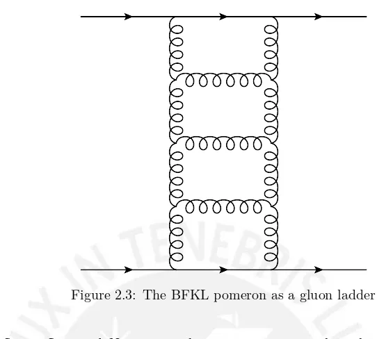
Figure 2.3: The BFKL pomeron as a gluon ladder
Later, Low and Nussinov make an attempt to explain the nature of the pomeron in terms of QCD fundamental constituents by proposing a model in which the pomeron is viewed as a two-gluon exchange, which is the minimum number of gluons able to produce a colorless combination.
In general the two gluons could couple either to the same quark or different quarks in the colliding hadrons. The latter case is incompatible with the photon like interaction between quarks and pomeron proposed by Standoffish. However, if the gluon correlation length in the QCD vacuum is much smaller than the hadron radius, the diagrams where the gluon couple to different quarks are strongly suppressed. In this way non-perturbative effects establish a bridge between the two models.
In perturbative QCD, on the other hand, using the Balitsky Fadin Kuraev Lipatov (BFKL) equation the pomeron can be pictured as an exchange of gluon ladders as shown in fig. 2.3. This leads to a hard pomeron with intercept
αhardP ≃1.5forαs= 0.2.
2.3 Diffraction
In a general way, diffraction can be defined in the following terms:
A reaction in which no quantum numbers are exchanged between the colliding particles is, at high energies, a diffractive reaction
This definition is simple and general enough to cover all cases:
I elastic scatteringwhen exactly the same incident particles come out after the collision.
1 + 2→1′+ 2′
2.4. KINEMATICS OF DIFFRACTION 21
resonance) with the same quantum numbers.
1 + 2→1′+X
2
III double diffractionwhen each incident particle gives rise to a bunch of final particles (or resonance) with the same quantum numbers of the two initial particles
1 + 2→X1+X2
IV central diffraction when the same incident particles came out after the
collision but a central system is created that gives rise to a bunch of particles (or resonance) with the quantum numbers of the vacuum.
1 + 2→1′+X+ 2′
In the practice, however, it can be difficult to prove that the only exchanged quantum numbers were those of the vacuum if the final states were not com-pletely reconstructed.
Then it is convenient to give an operational definition of diffraction as follows:
A diffractive reaction is characterized by a large non-exponentially suppressed rapidity gap in the final state
Rapidity gaps can also occur in non-diffractive events due to multiplicity fluctuations but the number of these event are exponentially suppressed. If we denote by∆η the rapidity gap of the final state, the distribution of diffractive
events is
dN
d∆η ∼constant (2.3.1)
While for non-diffractive events is
dN
d∆η ∼e
−∆η (2.3.2)
2.4 Kinematics of diffraction
In the following we review briefly the kinematics of diffraction scattering and the production of rapidity gaps. Lets first define some quantities:
2.4.1 Important physical quantities
The rapidity of a particle with momentum p = (px, py, pz) and energy E is
defined as:
y=1
2ln
[
E+pz
E−pz
]
(2.4.1)
and its pseudorapidity is given by:
η=1
2ln
(
|p|+pz
|p| −pz )
.. p1
. p2
.
p3
.
p4
[image:34.595.147.500.112.649.2]. θ
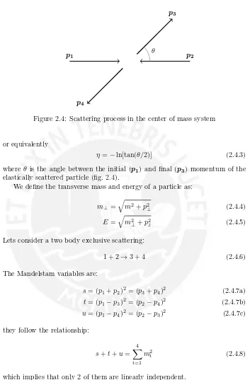
Figure 2.4: Scattering process in the center of mass system
or equivalently
η=−ln[tan(θ/2)] (2.4.3)
where θ is the angle between the initial (p1) and final (p3) momentum of the
elastically scattered particle (fig.2.4).
We define the transverse mass and energy of a particle as:
m⊥=√m2+p2
⊥ (2.4.4)
E=√m2
⊥+p2z (2.4.5)
Lets consider a two body exclusive scattering:
1 + 2→3 + 4 (2.4.6)
The Mandelstam variables are:
s= (p1+p2)2= (p3+p4)2 (2.4.7a)
t= (p1−p3)2= (p2−p4)2 (2.4.7b)
u= (p1−p4)2= (p2−p3)2 (2.4.7c)
they follow the relationship:
s+t+u=
4 ∑
i=1
m2i (2.4.8)
which implies that only 2 of them are linearly independent. Lets remember briefly that:
s= (p1+p2)2
s=p21+p22+ 2p1p2
2.4. KINEMATICS OF DIFFRACTION 23
but in the C.M. systemp1=−p2 so:
s=m21+m22+ 2E1E2+ 2p1p1
s=m21+m22+ 2E1E2+p21+p22
s=m21+p21+m22+p22+ 2E1E2
s=E12+E22+ 2E1E2= (E1+E2)2
And since the total energy of the system isE=E1+E2, we have, in the center
of mass system (CMS):
ECMS=√s (2.4.9)
2.4.2 Diffractive scattering and rapidity gaps
Lets now consider the scattering process:1 + 2 = 3 +X
referring to the collision of two particles of mass m (1 and 2), one of them
experiencing elastic scattering (3), and the other becoming an excited state
system of massMX which then fragments into a cascade of particles represented
byX.
In the center of mass system we have,
p1= (E1,p)
p2= (E2,−p)
p3= (E3,p′)
then, from momentum conservation,
(p1+p2)2= (p3+pX)2
s= (p3+pX)2
=p23+p2X+ 2p3pX
=m2+MX2 + 2E3EX−2p3pX but againp3+pX = 0andE=E1+E2=E3+E4=√s, so:
s=m2+MX2 + 2E3EX+ 2p2X
=m2+MX2 + 2E3EX+ 2(EX2 −MX2)
=m2−MX2 + 2EX(E3+EX)
=m2−MX2 + 2EX(√s)
⇒EX =
s−m2+M2
X
2√s (2.4.10)
From here is easy to see, usingE3=√s−EX, that:
E3=
s+m2−M2
X
In the limit when s, MX2 ≫m2:
EX ≃
s+MX2
2√s (2.4.12)
E3≃
s−M2
X
2√s (2.4.13)
Under this approximation, and squaring eq. (2.4.12), we find the momentum |p′|
EX2 =MX2 +p2X= s
2+ 2s2M2
X+MX4
4s
4sp2X=s2−2s2MX2 +MX4 p2X= (s−M
2 X)2
4s
|pX|=|p′|= (s−M
2
X)
2√s (2.4.14)
For a very fast particle with momentump(pz→ ∞) and energyEits rapidity
is:
y=1
2ln
(
E+pz
E−pz
)
Multiplying by(E+pz)/(E+pz)and operating:
y= 1
2ln
(
(E+pz)(E+pz)
(E−pz)(E+pz) )
= 1 2ln
(
E2+ 2Epz+p2z
E2−p2
z ) = 1 2ln ( m2
⊥+ 2Epz+ 2p2z
m2⊥
)
= 1 2ln
(
1 +2pz(E+pz)
m2
⊥
)
Sincepz→ ∞ ⇒ pz≫m ∧ E≃pz, then
y≃ 12ln
(
1 + 4p
2 z
m2⊥
)
≃ 12ln
(4p2
z
m2⊥
) =ln (2 pz m⊥ ) (2.4.15)
Using eq. (2.4.15) for the scattered particle in the diffractive process (with energy
E3 and momentump′):
y=1
2ln
(
E3+p′z
E3−p′z
2.4. KINEMATICS OF DIFFRACTION 25 .. ln( M2 m2 ) . ln( s
M2
)
.
ln√m s
.
ln M2
m√s
.
ln√s m
Figure 2.5: Rapidity gap in the single diffractive process1 + 2→3 +X
At large √s, considering particle 3 as the result of the scattering of 1, and
p′
z>0,
y≃ln
( 2
m⊥
(
s−MX2
2√s ))
≃ln
(√s
m⊥ −
M2
X
m⊥√s
) ≃ln (√ s m⊥ ) (2.4.17)
The maximum rapidityy attainable for particle 3 is reached whenp⊥= 0:
ymax≃ln
(√s
m )
(2.4.18)
For the diffracted system of mass MX by the previous discussion we may
expect that if we have all the mass MX concentrated in just one particle its
rapidity will be be
⟨yMX⟩=ln( √
s/MX) (2.4.19)
Due to its compositeness, there will be a distribution in rapidity for the particles originating from this system, the maximum (in absolute value) occurring for a particle of transverse mass∼mand momentum∼√s/2
|yX|max≃ln
(√
s m
)
(2.4.20)
whereas the minimum value of |yX| pertains to a particle with momentum
∼(m/M)√2 and transverse mass∼M,
|yX|min≃ln (
m√s
M2
)
(2.4.21)
Then the rapidity gap between particle 3 and the edge of the rapidity distribu-tion of the systemX is roughly given by
∆y≃ln
(√ s m ) +ln (
m√s
M2
)
=ln( s
M2
)
Chapter 3
The AD detector system
3.1 Introduction
As mentioned in the previous chapter, diffractive events can be tagged using pseudorapidity gaps. In order to design effective triggers that can select those events it is important to know their general properties, among them the pseu-dorapidity distribution of these class of events. For this we will use two Monte Carlo generators, Pythia6[19] and Phojet[8], that implement different models of diffraction and can be used to estimate these distributions.
Before continuing, some conventions will be introduced. The frame of refer-ence for the ALICE experiment is as follows: the positive y axis coincide with
the upward direction. The positive x axis is parallel to the horizontal plane
and points towards the LHC center. The positivez axis is also parallel to the
horizontal plane and its direction is such as to form right handed coordinate system. The origin of coordinates is located at the nominal interaction point. The planez= 0divides the experiment in two sides, left or C side (z <0) and
right or A side (z >0). The ALICE convention dictates that the letters A or C
are appended to the name of sub-detectors to denote their location.
In single diffraction events, any of the two colliding protons can break up, while the other remains intact. In what follows we designate as single-diffractive-left (SD-L) events, those in which the proton that breaks up goes to the direction of the negativezaxis (i.e has momentumpz<0) or to the left side. Accordingly,
events in which the proton that breaks up goes to the right side (pz >0) are
denoted single-diffractive-right (SD-R).
Single diffraction events have a characteristic particle distribution. Let us consider the case for SD-L. The charged particle distribution dNch/dη has a
notorious peak at forward pseudorapidities at η ≈ −5, corresponding to the
fragmented proton, and a smaller peak atη ≈ −10 due to the surviving
(non-diffracted) proton (fig. 3.1, top). A symmetrical distribution can be found if we exchange the direction between the diffracted and the non-diffracted proton. Double diffraction (DD) happens when both protons become excited and un-dergo break up. These events present two symmetric peaks at forward rapidities and a dip around η = 0 (fig. 3.1, bottom left). In central diffraction (fig.3.1,
bottom middle) both protons survive (small peaks atη≈ ±10) but they create
a diffracted mass which involves various particles at central rapidities (central
peak atη= 0). The non-diffractive events (ND) do not exhibit pseudorapidity
gaps (fig.3.1, bottom right).
As it has been seen in the previous chapter the individual characteristics of single diffractive events are determined by the energy of the collision and the diffracted mass (MX). In particular for high masses the gap size is
ap-proximately ∆η ≈∆y ≈ ln(s/M2
X). The collision energy
√
s is fixed by the
experiment while the diffracted mass follows an exponential distribution of the form 1/MXf(∆). Here ∆ = αP −1 with αP the intercept of the pomeron
tra-jectory. The exact form of f depends on the Regge trajectories considered in
the Feynman diagram. The uncertainty in the knowledge of this distributions constitute the main contribution to the systematic error in diffractive physics. In fig. 3.2 the probability of having an SD-L event, according to Pythia and Phojet, as a function of the mass of the diffracted system (MX), is plotted.
It has been observed at the Tevatron (√s= 1.8 TeV) that the contribution
of diffractive processes represent about 25% of the total inelastic cross section[2] for proton-antiproton. From the previous chapter we know that the cross section of diffractive processes grows as ln(s), thus, it is expected that the diffractive
processes, at the LHC energies, contribute significantly to the total inelastic cross section. In this way, our accurate knowledge of the size of the contribution of the diffractive processes in the inelastic sample, is critical for measuring, with very good precision, the different LHC observables.
In figure 3.1we observe that the ALICE detectors mostly cover the central pseudorapidity range, for instance, the both layers of SPD are within|η|<2.0
and the TPC is in the range of|η|<0.9. This coverage is complemented by the
FMD and VZERO detectors which extend the ALICE pseudorapidity range to
−3.7< η <5.1. Using the SPD, FMD and VZERO we are able to select about
3.1. INTRODUCTION 29
η
-10 -5 0 5 10
η dN/d 0.00 0.05 0.10 0.15 0.20 0.25 0.30 0.35 0.40 0.45 0.50
SD-L
η-10 -5 0 5 10
η dN/d 0.00 0.05 0.10 0.15 0.20 0.25 0.30 0.35 0.40 0.45 0.50 DD η
-10 -5 0 5 10
η dN/d 0.00 0.05 0.10 0.15 0.20 0.25 0.30 0.35 0.40 0.45 0.50 CD η
-10 -5 0 5 10
[image:41.595.116.440.140.588.2]η dN/d 0.00 0.05 0.10 0.15 0.20 0.25 0.30 0.35 0.40 0.45 0.50 ND
![Figure 1.2:The Time Projection Chamber of ALICE. Left: Schematic view(from [6]). Right: Tracks reconstructed by TPC in a Pb-Pb event.](https://thumb-us.123doks.com/thumbv2/123dok_es/2405541.15804/15.595.109.438.320.490/figure-projection-chamber-alice-schematic-right-tracks-reconstructed.webp)
![Figure 1.9: Elliptic flow as seen by ALICE. From [21]](https://thumb-us.123doks.com/thumbv2/123dok_es/2405541.15804/27.595.103.443.247.459/figure-elliptic-ow-seen-alice.webp)