Universidad Nacional de La Plata
Novenas Jornadas de Economía
Monetaria e Internacional
La Plata, 6 y 7 de mayo de 2004
Crises and Crashes: Argentina 1885–2003
Please do not quote This draft: April 2nd, 2004
Comments welcome
C
CR
R
I
I
S
S
E
E
S
S
A
A
N
N
D
D
CR
C
R
A
A
S
S
H
H
E
E
S
S
:
:
AR
A
R
G
G
E
E
N
N
T
T
I
I
N
N
A
A
1
1
8
8
8
8
5
5
–
–
2
2
0
0
0
0
3
3
.
.
Ana María CerroUniversidad Nacional de Tucumán [email protected]
Osvaldo Meloni
Universidad Nacional de Tucumán [email protected]
Abstract
The objective of this paper is to study the economic history of crises in Argentina. Following Prebisch´s conjecture, we look for regularities in the behavior of key macroeconomic variables in the neighborhood of the crises. We perform parametric and non-parametric analysis in order to determine whether the Argentinean crises respond to the predictions of first, second or third generation models.
Firstly, we identify crises episodes throughout the Argentine history from 1885 to the present. We apply the Eichengreen, Rose and Wyplosz (1994) methodology to sort crises from non-crises periods, and we distinguish among deep non-crises (crashes), mild non-crises and turbulent episodes. Secondly, we split the sample in crises and non-crises years and carried out graphical analysis, and not parametric tests in order to establish weather key macroeconomic variables, namely public expenditure, GDP, external debt, exports, imports and the current account deficit change significantly before, during and after crises. We report the two-sample Kolmogorv-Smirnov test of equality of distributions and the Kruskal-Wallis test of equality of population.
Since the previous studies are intrinsically univariate, we also performed a regression analysis, estimating a logit model. It is found that fiscal variables have an important role in determining the probability of crisis. The domestic macroeconomic effects, measured by GDP growth and real M3 growth are also very strong. An appreciation of the currency (lagged once) also increases the probability of a crisis. We can also see that an impairing of external conditions make a crisis more probable.
Crises and Crashes: Argentina 1885 – 2003.
Ana María Cerro and Osvaldo Meloni*
Universidad Nacional de Tucumán - Argentina E-mail: [email protected]
La crisis actual es la misma de 1870, la de 1865, la de 1860, de la 1852, de la 1840, etc. El país ha vivido en esas crisis desde que dejó de ser colonia de España. Podría decirse que no es económica sino política y social. Reside en la falta de cohesión y de unidad orgánica del cuerpo o agregado social que se denomina Nación Argentina, y no es sino un plan, un desideratum de nación. La diversidad y lucha de sus instituciones de crédito, la anarquía de sus monedas, la emulación enfermiza que preside a sus gastos dispendiosos en obras concebidas para ganar sufragios y poder, vienen del estado de descomposición y desarreglo en que se mantienen las instituciones, los poderes, los intereses del país.
Juan Bautista Alberdi Escritos Póstumos. Estudios Económicos. Tomo I.
En la historia monetaria argentina, a pesar de su confusa apariencia, nótese una serie de períodos de ilimitada confianza y prosperidad, de expansión en las transacciones, de especulación inmobiliaria y fantasía financiera, seguidos de colapsos más o menos intensos, precipitados en pánicos que originan la liquidación forzada de las operaciones, el relajamiento de la confianza, la postración y el estancamiento de los negocios. Sin duda, cada uno de estos ciclos no se presentan exactamente en las mismas condiciones, ni con idéntico carácter, pero, considerados en conjunto, es posible encontrar en ellos, hechos fundamentales que se repiten, cuyo análisis permite formular síntesis acerca de su evolución... buscaremos demostrar que en nuestras crisis, aparte de las diferencias de menor cuantía, interviene un factor fundamental, ...y peculiar al grado de formación histórica del país.
Raúl Prebisch Anotaciones sobre nuestro medio circulante (1921)
En los últimos 15 años, la Argentina ha gastado mucho más de lo que producía, omitiendo reponer las inversiones básicas de capital y endeudándose fuertemente en el exterior. ... Más del 80% de los ingresos del Estado se va en sueldos, y ello explica que no haya dinero para hacer viviendas, ni caminos, ni escuelas, ni siquiera para reparar pavimentos o dar más luz a nuestras obscuras calles... La Argentina ha estado viviendo una ficción económica, cuyas consecuencias están claramente a la vista...Todos los gobiernos han coincidido en la necesidad de reducir los elencos administrativos y las crecientes pérdidas de los servicios públicos, pero año tras año, esos gastos y esas pérdidas han ido en aumento ...
Arturo Frondizi Radio Speech to the People of Argentina. Memoria Anual 1958, Banco Central de la República Argentina.
*
I
I.. IINNTTRROODDUUCCTTIIOONN
Social sciences researchers faced to the Argentinean economic history for the first time, usually get surprised by the repetitiveness in economic episodes1. Those that deepen the study get
absolutely astonished. Some economic events, like crises, seem to come and go over and over again. As sustained by former central banker Raúl Prebisch, more than 80 years ago (see quotation), characters may change, characteristics might be different but some fundamental facts can be traced throughout history. Why crises are so frequent and of such large magnitude? What are these crises caused by? Do they always recognize the same causes? Which are those “fundamentals” named by Prebish? Juan Bautista Alberdi and Arturo Frondizi, from different centuries and positions, blamed the irresponsible fiscal policy for the ever-returning crisis in the country (see quotation). However, external factors and expectations about the sustainability of economic policy might have played a role in the crises.
Case studies focused on particular crisis, like della Paolera and Taylor (1999, 2000) that analyze the 1929-32 crisis, seem to confirm the importance of the fiscal link in the crisis, although they stress too other factors like poor regulated financial sector and adverse external conditions. Similar conclusions can be drawn from numerous papers that study more recent crises (See Dornbusch, 1984; Cumby and van Wijnbergen, 1989; Kehoe, 2003; and Veigel, 2004).
The objective of this paper is to study the economic history of crises in Argentina. Following Prebisch´s conjecture, we look for regularities in the behavior of key macroeconomic variables in the neighborhood of the crises. We perform parametric and non-parametric analysis in order to determine whether the Argentinean crises respond to the predictions of first, second or third generation models.
Firstly, we identify crises episodes throughout the Argentine history from 1885 to the present. We apply the Eichengreen, Rose and Wyplosz (1994) methodology to sort crises from non-crises periods, and we distinguish among deep non-crises (crashes), mild non-crises and turbulent episodes. As far as we know, there are no comprehensive studies on argentine crises for long periods of time, covering the XIX and XX century as well as the present23
.
1
Excessiveness is also an outstanding feature of Argentina’s economic life. Periods of euphoria and unlimited enthusiasm are followed by frustration and endless delusion without any transition time (see Prebish’s quotation)
2 Studies like those of the Bordo and Vegh (1998) and Saxton (2003) cover long periods of time but their emphasis is different from ours.
3
Secondly, we split the sample in crises and non-crises years and carried out graphical analysis, and not parametric tests in order to establish weather key macroeconomic variables, namely public expenditure, GDP, external debt, exports, imports and the current account deficit change significantly before, during and after crises. We report the two-sample Kolmogorv-Smirnov test of equality of distributions and the Kruskal-Wallis test of equality of population.
Since the previous studies are intrinsically univariate, we also performed a regression analysis, estimating a logit model. The analysis of the macroeconomic variables in the neighborhood of
the crises also helps us to test the validity of Alberdi’s hypothesis as well as determine whether they respond to the predictions of the first or second-generation models of currency crises. This is particularly important since policy prescriptions are different depending on the type of crisis faced by the country.
The remainder of the paper is organized as follows. Section II sketches some theoretical issues on BOP crises. In Section III we construct a market turbulence index for the 1823 – 2002 period that allows us to identify crises episodes and classify them as deep, mild and minor turbulence. Section IV describes the behavior of macroeconomic variables in the neighborhood of the crisis and the historical context of each crisis. Section V explains the results obtained from the non-parametric tests carried out. Finally, section VI presents some conclusions, conjectures and guidelines for further research.
I
III.. TTHHEEOORREETTIICCAALLBBAACCKKGGRROOUUNNDD
Since Krugman (1979) developed the first canonical model of currency crisis, a great deal of theoretical and empirical literature has surged. Most of the theoretical literature was concerned with the conditions a crisis should fulfilled in order to be considered first, second and/or third generation crisis, while most of the empirical studies tried to identify crises across countries according to this classification.
F
FIIRRSSTTGGEENNEERRAATTIIOONNMMOODDEELLSS
Krugman’s seminal paper (1979) showed how inconsistencies between domestic economic conditions and the exchange rate commitment led to the collapse of the currency peg. In his paper, budget deficit fully monetized was financed by Central Bank expending reserves. When such reserves fell to a critical threshold a speculative attack was launched, causing reserves depletion and the abandon of the exchange rate peg.
through the operation of international agencies buying and selling commodities. On theoretical grounds, such scheme would be subject to important speculative attacks. The underlying logic of the model described by Salant and Henderson was taken by Krugman, and refined by Flood and Garber (1984), to explain central banks attempts to stabilize the exchange rate.
In the canonical currency crisis model, currency crises are the result of the fundamental inconsistency between domestic policies –generally the persistence money-financed budget deficit- and the attempt to fix the exchange rate. This inconsistency may be sustained while Central Bank has sufficiently large amount of reserves, but when reserves reach enough low level, speculators force currency crises.
Since government fixes the exchange rate, investors wish to hold domestic and foreign assets in fixed proportions. They rebalance their portfolio by exchanging domestic for foreign reserves of the central bank, since there is no internal mechanism to get rid of the excess money supply. If speculators were to wait until financing the deficit depletes reserves, they would realize that holding foreign exchange is more attractive than domestic currency, leading to a jump in the exchange rate. But since agents are rational, no jump is possible, so they would sell domestic currency before the depletion of reserves, leading speculator to sell even earlier. The speculative attack takes place when the shadow price of exchange rates (the price that would prevail after the speculative attack takes place) equals the exchange rate. At that moment reserves are driven to zero forcing the abandonment of the fixed exchange rate, and the economy switches to a floating rate regime. With reserves depleted, budget deficit is financed by money creation, which in turn causes an increase in inflation rate.
Two important aspects of this model should be highlighted: the first one is that many economies reflect a basic inconsistency between fiscal policy and exchange rate regime. In this framework, speculative attacks are not only possible, but also inevitable. The time in which it will take place is perfectly known forehand, so nobody is taken by surprise. Secondly, even attacks may appear arbitrary and capricious, they can occur in a world where all speculators are completely rational. Rational economic behavior, characterized by smoothly evolution over time, can be associated with dramatic attacks and changes in the exchange rate regimes.
S
SEECCOONNDD--GGEENNEERRAATTIIOONN MMOODDEELLSS
After the canonical crisis model failed to explain the European Monetary System crises (1992-1993), new generations of crisis models arose. The so– called second generation models developed by Flood and Garber (1984b) and Obstfeld (1986, 1994) focused on government comparison of the net benefits from changing the exchange rate versus defending it.
The new generation models are based on the existence of multiple equilibria. When investors, while not questioning that currency policy may be consistent with the currency peg, they anticipate that a successful attack will alter policy, so it is expected future fundamentals, conditional on an attack’s taking place, which are incompatible with the peg. In this case government might defend the currency, but the costs (high interest rate, high unemployment rate) can be so high that government finally devaluates, so market anticipate that action and acts in advance.
The government has so many good reasons to abandon the fixed exchange rate as to defend it. But the cost of defending a fixed exchange rate increases when people expect that the regime will be abandoned.
There might be several reasons why government wishes to abandon fixed exchange rate. For example, if government has a large debt burden denominated in domestic currency, devaluation would evaporate part of the debt. Or, if the country is suffering high unemployment rates, and nominal wages are rigid, devaluation would diminish real wages.
If government has reasons to devaluate, why it would defend fixed exchange rate? One reason in inflation-prone countries is that a nominal anchor is a guarantee against high inflation rates. It is also argued that a fixed exchange rate facilitates investment and international trade. Finally it might be considered as a strong commitment to international cooperation (the case of Sweden in 1992)
T
THHIIRRDD GGEENNEERRAATTIIOONN MMOODDEELLSS
The standard explanation for speculative attacks had serious shortcoming when applied to the recent Southeast Asian currency crisis in 1997. The conventional currency crisis theory associated with inconsistency in present or future fundamentals missed important aspects in the Asian crisis.
Every crisis is different, but the Asian crises seem to differ from the standard theory in several fundamental ways. We are specifically referring to the role played by financial intermediaries whose liabilities were perceived to have government guarantee, but were essentially unregulated and therefore subject to moral hazard problems.
In first generation model a la Krugman the collapse is inevitable and is the result of an over expansive fiscal policy, which is inconsistent with the monetary policy. In second generation models, crisis are the result of the predicted impair in fundamentals, or purely the result of self fulfilling prophecy.
Despite every crisis is different, Asian crises differed from traditional crisis in many ways as Krugman (1998) points out. First, none of the fundamentals that led to crises a la Krugman were present in the Asian economies. Second, Asian economies did not face severe unemployment when the crisis begun, nor had any incentive to abandon the peg to carry out expansive monetary policy. Third, in all countries were present a boom-bust cycle in the asset markets. Finally financial intermediaries had a central role in the crisis. A mismatch in the deposits of the banking and non-banking system was present: the institutions borrowed short term money, often in foreign currency, and lent that money in long term domestic currency.
The evidence seems to suggest that Asian crisis was neither the consequence of fiscal imbalances, nor were the incentives to follow an expansive monetary policy, but were the problems with financial intermediaries that drove the crisis. The excessive risk lending led to inflation in the asset prices. When the crisis burst, the asset prices fall, the insolvency of intermediaries were visible, forcing them to cease operations, which in turn implied further deflation in asset prices.
I
IIIII EEMMPPIIRRIICCAALL LLIITTEERRAATTUURREE
On the other hand, second generation models imply that speculative attacks should be followed by expansive monetary and fiscal policies.
Third generation models emphasize in the role played by financial intermediaries, so they analyze variables related to them, such as the liquidity coefficient, solvency of the financial sector, external debt maturity, and assets denomination versus liabilities.
Blanco and Garber (1986) using a variant of Krugman-Flood and Garber model, find important insight related to the behavior of macro variables previous, during and after the crisis. It predicts that we should not only observe fiscal deficit, but also growing quantity of money, wages, real exchange rate appreciation, impairing in current account deficit and in the trade balance and an increase in the domestic rate of interest. This work was extended by Goldberg (1993) and by Cumby and van Wijnbergen (1989) for the crawling peg experience in Argentina during the 80's.
These papers focused on specific events and on particular countries. Later studies concentrated upon cross-countries crisis episodes. For example Edwards (1989) studies 39 devaluation in emerging countries during 1962 -1983.
The speculative attack during the 90's challenged the view of researchers that crises respond to irresponsible fiscal and monetary policy. Empirical papers tried to understand the origins of these crises. They studied the behavior of macro and financial variables during crisis episodes and compared with tranquil periods. Eichengreen, Rose and Wyplosz (1995), Sachs, Tornell and Velasco (1996), and Kaminsky, Lizondo and Reinhart (1997) followed this line of research. The severe crisis in Southeast Asian countries (1997), opened a new branch of investigation. Most papers tried to emphasize in the role of financial variables to explain crises. For example McKinnon and Pill (1998) compare the Southeast Asian crises with the episodes in Mexico and Chile, finding important similarities but they point out that the Asian episodes were exacerbated by the unhedged foreign exchange position of Asian banks.
I
IVV IIDDEENNTTIIFFYYIINNGG CCUURRRREENNCCYY CCRRIISSEESS
There is not a unique definition of currency crisis, however most economists would agreed that a currency crisis is an speculative attack against currency that ends up in a devaluation if the attack is successful. However authorities may ward off the attack by losing huge amount of foreign reserves and/or by increasing the rate of interest.
One of the key questions to be solved in the analysis of crisis is how to identify speculative attack in foreign exchange rate, and to settle under what circumstances the movement in these indicators represents a crisis. The following issues arise: Should currency crisis be limited to exchange rate devaluation, how large a movement must be to be considered a crisis, and in high inflation periods, how large a devaluation must be to qualify for a crisis.
Frankel and Rose (1996) construct the most obvious indicator of crises: changes in the nominal exchange rate, on the grounds that foreign reserve data contains a lot of noise, and few countries have market-determined short-term interest rates. They also point out that if speculative attack is successful, it ends up in currency devaluation, and that is the case in most emerging countries.
Some researchers have proposed indexes that weight different components of speculative attack. However in some cases they are not easy to construct, as is the case in Girton and Roper (1979)
Eichengreen et al (1994) propose a weighted index of speculative attack component weighting by the inverse of the variability of each component to ensure that the units are comparable. They include in the currency crisis definition changes in the exchange rate, in the international reserves and in the interest rates. As Moreno and Trehan (2000) point out there is an implicit assumption in this approach that a one standard deviation change in the interest rate represents as much of a currency crisis as a one standard deviation change in exchange rates or reserves. Many researchers followed a similar methodology. For example Kaminsky and Reinhart (1999) construct a similar index, but they exclude interest rate on the ground that it is not consistently available for the whole sample they use.
In high inflation episodes, rates of depreciation are consequently high. To ensure we do not consider each of these deprecations as an independent crisis, it is necessary to compute separate standard deviations for those periods. As pointed our by Reinhart and Kaminsky (1999), if standard deviation is computed for the full sample, too many crises may be identified during inflationary episodes.
From the discussion we see that no measure of currency crises is perfect, they all have pros and cons, and there are always elements of arbitrariness.
In this study we focus on Argentines crisis for the period 1885-2003. We opted for an index similar to the one proposed by Eichengreen et al (1994) and Kaminsky and Reinhart (1999)4, to
capture episodes like Tequila, where authorities managed to keep the peg, despite the lose in reserves and the increase in interest rate, as we are interested in all speculative attack, successful or not. Afterwards and in according to the value of the index, we will classify the episodes as deep, mild and turbulent crisis.
The index stems from the idea that market pressure increases when exchange rate devaluates (rises), when interest rates increase and when international reserves fall. Under a floating exchange rate regime, we expect abrupt increases in the exchange rate as crisis develops, while under a fixed exchange rate, prior to devaluation, interest rates increase and international reserves diminish.
We use the rate of change of nominal interest rate rather than the difference between the domestic and international rate, as in other papers, due to the inflationary process Argentina went through during the centuries. These inflationary processes implied high and volatile rate of interest, and given the relative constancy of the international rate, the difference between domestic and international rate proved to be meaningless to capture turbulent periods, so the rate of change is a better definition. The Market Turbulent Index (MTI) is:
4
We also included the rate of interest in the index but not for the whole period since this series is not available monthly
σ
σ
σ
σ
σ
σ
e R ii
R
e
Where the symbol ∧∧ represents the growth rate of the variable, e is the exchange rate, R stands for international reserves, i is the domestic interest rate and σσe, σσR, σσi are the standard
deviations of the growth rate of the exchange rate, international reserves and domestic interest rate, respectively.
The Index is weighted by the inverse of the respective standard deviation to avoid the most variable component dominates the index movements. However, we also used different weights to test the robustness of the index, and the crisis determination proved to be quite robust to different weight specifications.
The index was computed with monthly data from 1914 to 20025. We imposed different criteria
to sort crises, but whenever the MTI is greater than the mean plus k standard deviation we identify a “signal” or “turbulent episode”.
We require at least two “close” months with MTI greater than three STD to consider that
episode as deep crisis or "crash". If the MTI is greater than two STD but less than three STD,
we call it “mild crisis”. If MTI exceeds its mean value in a half STD at least twice the episode is
considered “minor turbulence”. The remaining episodes, i.e. when the index departs less than one half standard deviation from the average are termed as “non- crisis” or tranquility times. In high inflation episodes (1976 and 1989), we excluded the data for the estimation of the moments, to avoid these data distort the moments.
[image:12.612.101.457.498.629.2]In order to determine the boundaries of a given crisis and so avoiding dating twice the same crisis, we require at least six months with no signals between each other.
Table 1. Criteria to sort Crises
Monthly Data
Criteria
Index # of Signals Classification
MTI < 0.5 σMTI Non- crisis
0.5 σMTI<MTI< 2 σMTI Two close months Minor Turbulence
2 σMTI <MTI < 3 σMTI Two close months Mild
MTI > 3 σMTI Two close months Deep
The MTI was computed for five sub periods in order to keep its variance relatively
hyperinflation with the consequent impact on exchange rates and international reserves. So we treat those periods separately to avoid excluding crises episodes that could appear as
tranquility times when compared with hyperinflation periods. The sub periods chosen were the
following:
(a) From Roca to the First World War: 1885-1913 (b) The Interwar Period: 1914- 1945
(c) From Perón to Perón: 1946- 1976
(d) From Hyper to Hyper Inflation: 1976- 1991 (e) Convertibility: from boom to burst: 1992 – 2002
It is worth remark that the terms “tranquility”, “minor turbulence”, “mild” and “deep” are referred to the sub period considered and is not intent to be an absolute qualification for the whole period.
D
DAATTAA
Considerably effort has been devoted on the construction of time series for 117 years. The market turbulence index was computed from monthly data from 1914 to the present. Exchange rates were taken from Vázquez- Presedo (1971 and 1975), Ámbito Financiero (1984) and FIEL. To construct the international reserves series we use data from Vázquez- Presedo (1971 and 1975) Internat ional Monetary Fund and Banco Central de la República Argentina (BCRA). Interest rates were taken from Vázquez-Presedo (1971 and 1975), FIEL and BCRA. Monetary, fiscal and international trade variables were obtained from Cortés Conde (1989) and also from BCRA, Ministerio de Economía de la Nación, Vázquez-Presedo and from Gerchunoff and Llach (2003). Recent data of terms of trade as well as exports and imports comes from CEPAL.
T
THHEE CCLLAASSSSIIFFIICCAATTIIOONN OOFF CCRRIISSEESS
We dated 19 crises throughout 117 years of history6.
Five crises were rated as “deep”, nine as
“mild” and five as “minor turbulence”. Interestingly, the number and magnitude of the crises
increases through time (see Table 2). The four “deep crises” identified correspond to the years, 1890-91, 1929-32, 1975-76, 1989-91 and 2001-02.
5 For the period 1980-1914 we used annual data 6
Table 2. Crises Summary
Type of crisis Period Years
(1)
Number of crises
(2)
Number of crises years (3)
Crises Years as % of total years (3)/(1)
GDP Growth (annual
average in%) Deep Mild
Minor Turbulence
1885-1913* 28 2 3 10 5.4 1 1
1914 -
1945 32 4 7 22 3.1 1 1 2
1946 –
1976 31 7 10 32 3.8 1 4 2
1977 –
1991 15 4 9 60 0.4 1 2 1
1991-
2003 11 2 3 27 2.1 1 1
Total 117 19 26 23 3.3 5 9 5
*We built the index for this period with annual data
The 19 crises implied 26 crises years. That is, Argentina was 23% of its 117 years in crises, which meant one crisis year every 4.5 years. A given year is considered a crisis year if the
market turbulence index exceeds one standard deviation from the average in at least 2 months consecutive or alternate.
According to our index, the most turbulent period of Argentina’s history was 1977 –1991, not only because it registered 4 crises in 15 years, but also because nine of those years were crisis
years, which meant 60% of these years in crisis(see Appendix, Table 2 A for details).
V
V MMAACCRROOVVAARRIIAABBLLEESS BBEEHHAAVVIIOORR IINN TTHHEE NNEEIIGGHHBBOORRHHOOOODDOOFFTTHHEECCRRIISSIISS
Differences in monetary and fiscal policy indicators during periods of crisis versus non crisis, may shed light on whether an expansionary monetary and fiscal policy may trigger speculative attack as in Krugman first generation model.
On the other hand some internal or external indicator may give a sign that the cost of maintaining the peg is too high for the government, leading to a shift in expectations that may trigger a speculative attack, as in second generation model. For example a high rate of unemployment or a current imbalance as suggested by Obstfeld (1994) and Drazen and Masson (1994)
We present a brief summary of the behavior of fiscal, monetary and external variables before, during and after “deep crisis”.
Before crises.
® With the sole exception of the 1929-32 crisis, the remaining “deep crises” had significant and persistent budget deficits in the years preceding each crisis episode. Remarkably, the years before de 1975-76 crisis show fiscal deficits around 8% of the GDP. Likewise, in the two years preceding the 1989-91 crisis, fiscal deficit averaged 5.5% of the GDP. A closer look at the fiscal history of Argentina shows that deficits were the norm and surpluses very rare: only the years 1920, 1993 and 2002 (see Figure 1).
® In all six “deep crises”, public expenditures as well as the real money aggregate M3 grew at very high rates in the years preceding the crisis.
® We also verify increases in the interest rates, worsening in trade and current account deficits and severe drainage of international reserves.
• During Crises.
® In the five cases for which we have GDP estimations, economic activity plunges and consequently imports diminish substantially, which in turn contributes to trade and current account adjustment.
• After Crises.
® In the years following crisis we also register a strong recovery in economic activity, and hence in imports, and the return to current account deficit.
Figure 1. Budget Deficit and Crises 1883 -2002
Source: Gerchunoff and Llach (2003) and own calculations.
V
VII EEMMPPIIRRIICCAALL RREESSUULLTTSS
The empirical analysis has two parts. In the first one we compare the behavior of macroeconomic and external variables during crises using as control group the same variables but during non crises periods, following the Eichengreen et al (1994) and Frankel and Rose (1996) methodology. We cover a period that span from 1885 up to 2002 for Argentina. We present the mean and standard deviation of the series in appendix. There can be seen important differences between crises and non-crises samples.
G
GRRAAPPHHIICCAANNAALLYYSSIISS
Each of the graphics portrays the movement in a variable of interest beginning three years before the crisis until three years afterwards. As Frankel and Rose (1996) point out, a graphical approach has advantages and disadvantages. Among the first, a graphical analysis imposes no parametric structure on the data, makes only a few assumptions that are necessary in inference statistics, and they are often more accessible and informative than tables with estimations of coefficients. On the other hand, they are informal, and intrinsically univariate.
-2.0 0.0 2.0 4.0 6.0 8.0 10.0 12.0 14.0
1914 1919 1924 1929 1934 1939 1944 1949 1954 1959 1964 1969 1974 1979 1984 1989 1994 1999
Real and Public Sector: we can clearly see differential behavior of series in the moment of the crisis and three periods before and after crisis. Public Expenditure growth reaches a maximum two periods before crisis, then decreases until one period before.
Note: intervals of u+-sigma
Monetary series behave differently during crisis and in its neighborhood. Inflation peaks during the crisis, real M3 growth decreases considerably during crisis, while external debt peaks one year before crisis.
External Sector: exports and imports reach a trough during crisis, however imports fall more than exports, leading to a surplus in trade balance. As most emerging countries, Argentina loses access to international capital market during crisis, so the current account improves during crisis.. -400 -200 0 200 400 600 800 1000
t-3 t-2 t-1 t t+1 t+2 t+3
Inflation -40 -30 -20 -10 0 10 20 30
t-3 t-2 t-1 t t+1 t+2 t+3
Real M3 Growth
-4000 -2000 0 2000 4000 6000
t-3 t-2 t-1 t t+1 t+2 t+3
Public External Debt (Changes)
-15 -10 -5 0 5 10 15
t-3 t-2 t-1 t t+1 t+2 t+3
GDP Growth -20 -10 0 10 20 30
t-3 t-2 t-1 t t+1 t+2 t+3
Public Expenditure Growth
0 2 4 6 8 10
t-3 t-2 t-1 t t+1 t+2 t+3
Fiscal Deficit (% of GDP)
-6 -4 -2 0 2 4
t-3 t-2 t-1 t t+1 t+2 t+3
Before crisis we observe an appreciation of domestic currency, which is reverted during crisis.
Terms of Trade peaks a period before crisis, which as we have already said, it let us think that in most severe crisis adverse external conditions were present . A similar behavior shows an international interest rate. This is an important for emerging economies for two reasons. The first one is pointed out by Calvo, Reinhart and Leiderman( 1992). They find that international rate of interest is a relevant factor for determine the capital inflow and outflow to emerging countries. The second one is related to the service of external debt: an increase in the rate of interest is associated with an increase in quasi fiscal deficit, worsening fiscal accounts.
MTI and its components, as we expect since we use to sort crisis, behave differently during
crisis than in the periods before and after.
N
[image:18.612.106.548.282.560.2]NOONN--PPAARRAAMMEETTRRIICCTTEESSTTSS
Tables 3 and 4 contain several statistical non-parametric techniques that allow a more systematic comparison between episodes. The first group of tests, that include Wilcoxon, Median Chi-square, Kruskal-Wallis and van der Waerden, are test of equality of population. They have as null hypothesis the equality of sample median among groups. The statistics tabulated are values of these tests under the null, so small values lead us not to reject the null
-400 -200 0 200 400 600 800 1000
t-3 t-2 t-1 t t+1 t+2 t+3
Crecimiento del Tipo de Cambio
-100 -50 0 50 100
t-3 t-2 t-1 t t+1 t+2 t+3
Crecimiento de las Reservas Interncionales
-2 -1 0 1 2 3
t-3 t-2 t-1 t t+1 t+2 t+3
Crecimiento del MTI
-0.10 -0.08 -0.06 -0.04 -0.02 0.00 0.02 0.04
t-3 t-2 t-1 t t+1 t+2 t+3
Current Account Deficit (as % of GDP)
0 40 80 120 160
t-3 t-2 t-1 t t+1 t+2 t+3 Terms of Trade
0 2 4 6 8 10
of equality of population. Small probabilities value computed let us reject the null (one asterisk indicate values less than 5%, while double asterisk less than 1%). We reject the null for all series, excepting CA and TOT, for all the methods reported.
Table 3. Panel A. Test of equality of population.
Method GDP Expenditure Public Revenue* Public Inflation M3
Wilcoxon/Mann-Whitney 3.8** 2.6** 3.6** 4.4** 2.6**
Med. Chi-square 9.6** 2.8** 11.7** 11.7** 2.3**
Kruskal-Wallis 14.5** 6.9** 13.1** 19.5** 6.8**
van der Waerden 14.3** 7.0** 13.7** 21.6** 8.4**
[image:19.612.103.523.619.690.2]Note: ** p-value less than 1%
Table 3. Panel B. Test of equality of population.
Method Exports Imports CA/GDP TOT
Wilcoxon/Mann-Whitney 2.51** 3.09** 0.91 1.87
Med. Chi-square 10.25** 7.08** 0.94 3.05
Kruskal-Wallis 6.31** 9.56** 0.83 3.53
van der Waerden 7.06** 10.16** 0.71 3.01
Note: ** p-value less than 1%
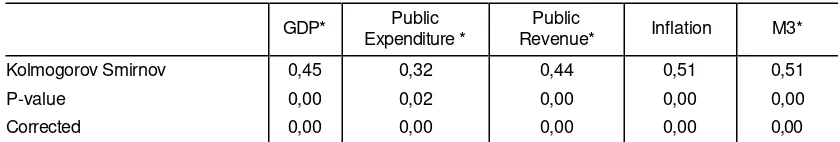
We also tabulated the two-sample Kolmogorv-Smirnov test for equality of distributions. This test is also a non-parametric one, and just like in tests of equality of population, small values of probabilities lead us to reject the null. Values computed are reported in Table 4.
According to the evidence presented, we are able to reject the null of equality of both population and distribution for the rate of change of public expenditure, income expenditure, M3, GDP, exports and imports (all in constant terms), and inflation. We are also able to reject the null for the rate of growth of exchange rate, reserves and the index. However this is not surprising since we are using these series as the criteria to determine crises versus non-crises episodes. We are unable to reject the null for CA and TOT, which is consistent with what we exposed before.
Table 4. Panel A. Kolmogorov- Smirnov Test.
GDP* Expenditure * Public Revenue* Public Inflation M3*
Kolmogorov Smirnov 0,45 0,32 0,44 0,51 0,51
P-value 0,00 0,02 0,00 0,00 0,00
Table 4. Panel B. Kolmogorov- Smirnov Test.
Exports* Imports* CA/GDP TOT
Kolmogorov Smirnov 0,36 0,42 0,14 0,12
P-value 0,01 0,00 0,71 0,88
Corrected 0,00 0,00 0,63 0,83
R
REEGGRREESSSSIIOONNAANNAALLYYSSIISS
The graphical and non parametric studies are intrinsically univariate. Now we use regression analysis, estimating a logit model since our dependent variable is binary, 0 for no crises years, and 1 for crisis years. In order to improve the contrast of the sample, we include deep and mild crisis event.
Among regressors we include 1) GDP growth, 2) public expenditure growth or fiscal deficit as % of GDP, 3) M3 growth, 4) real exchange rate overvaluation7
, 5) current account deficit as % of GDP, 6) terms of trade and 7) international rate of interest, 8) reserves as % of imports and 9) external debt.
We estimate logit models using maximum likelihood8. Results are tabulated in Table 5. Since
logit coefficient are not directly interpretable, we report the effect of a change in variables on the probability of crisis. We also tabulated z-statistics with null hypothesis of no effect. We also report McFadden R squared.
All the variables included have the correct sign coefficients, and most of them are statistically significative. A decrease in GDP growth, in real M3 growth, in the ratio reserves to imports, an appreciation of the peso (lagged once), and impairing of TOT (while not significative at standard values) increase the probability of crisis.
On the other hand an increase in public expenditure growth, in the current account deficit (lagged one period), in the external debt (not significative in Model 1), and an increase in the international rate of interest increase the probability of crisis.
Interestingly enough, the results of the regression let us conclude that fiscal variables have an important role in determining the probability of crisis. The domestic macroeconomic effects, measured by GDP growth and real M3 growth are very strong. An appreciation of the currency (lagged once) also increases the probability of a crisis, but contemporaneously it has the opposite sign as expected, since during crisis devaluation has already taken place. However
7
The degree of overvaluation of domestic currency is measured as the deviation from the trend 8
we can also see that an impairing of external conditions (measured by an increase in international rate of interest or by a worsening in TOT) makes a crisis more probable.
Table 6. Regression Results.
Variable Model 1 Model 2 Model 3
C 3.90
(1.18)
-0.93 (-0.27)
-0.85 (0.25)
GDP growth -0.17
(-2.99)
-0.17 (-2.76)
-0.17 (2.76)
Public expenditure growth 0.05
(2.55)
0.04 (2.29)
0.04
Real M3 growth -0.08
(-2.79)
-0.09 (-2.60)
-0.08 (2.60)
External Debt -6.05E-06
(-0.06)
1.45E-05 (0.13)
Terms of Trade (TOT) -0.06
(-2.10)
-0.03 (-1.14)
-0.03 (-1.18)
Current Account Deficit -4.90
(-0.78) -
Current Account Deficit (-1) 22.41
(-2.39)
-22.22 (-2.41)
LIBOR 0.23
(1.19)
LIBOR (-1) 0.56
(2.37)
0.55 (2.36)
Reserves /Imports -1.62
(-2.13)
-1.42 (-2.07)
-1.41 (-2.04) Real Exchange Rate overvaluation 0.41
(2.51)
0.44 (2.59)
0.44 (2.60) Real Exchange Rate overvaluati on (-1) -0.47
(-2.31)
-0.48 (-2.28)
-0.48 (-2.28)
LR statistic (11 df) 52.67285 60.28001 60.26328
Probability (LR stat) 8.56E-08 3.21E-09 1.19E-09
McFadden R-squared 0.42324 0.484366 0.484
Obs with Dep=0 92 92 92
Obs with Dep=1 26 26 26
I
IIIII.. CCOONNCCLLUUSSIIOONN
Alguna vez nos deja pensativos la sensación “de
haber vivido ya ese momento”.
Jorge Luis Borges,
La doctrina de los ciclos. En Historia de la Eternidad. Emecé Editores Buenos Aires 1998. Página 109
Since its independence, Argentina was involved in several crisis episodes. These episodes have been more frequent and deeper since 1930. Why crises are so frequent and of such large magnitude? What are these crises caused by? Do they always recognize the same causes? Why do governments, from different political parties, always get involved in large fiscal imbalances? What is the role of institutions?
This paper, does not aim to answer all these questions, but is aiming at understanding best Argentinean crises.
Firstly, we dated crises and classified them in “turbulent episodes”, “mild” and “deep”, by means of a Market Turbulence Index, defined as the weighed rate of change of exchange rate,
reserves and interest rates, for the period 1885-2002.
Secondly we perform parametric and non parametric analysis in order to determine whether the Argentinean crises respond to the predictions of first, second or third generation models.
We analyzed the behavior of macroeconomic and financial variables in the neighborhood of crises. We split the sample in crises and non-crises years and carried out graphical analysis, and not parametric test. In graphical analysis we observe that the behavior of key variables, namely public expenditure, GDP, external debt, exports, imports and the current account deficit changes significantly before, during and after crises.
We also report the two -sample Kolmogorv-Smirnov test of equality of distributions and the Kruskal-Wallis test of equality of population. We reject the null hypothesis of equal distribution and population.
These studies are intrinsically univariate, so we also performed a regression analysis, estimating a logit model. The results of the regression let us conclude that fiscal variables have an important role in determining the probability of crisis. The domestic macroeconomic effects, measured by GDP growth and real M3 growth are very strong. An appreciation of the currency (lagged once) also increases the probability of a crisis. However we can also see that an impairing of external conditions make a crisis more probable.
moment of explaining currency crisis. These let us say that crisis in Argentina share most of the characteristic of the first generation speculative attack models or a la Krugman. However we do not deny that elements of second and third generation models might be present as in Veigel (2004) and von Selzan (2003) for specific crises. But as far as we have studied, fiscal imbalances had a key role in explaining crisis. Our results seem to confirm Alberdi´s hypothesis that all the crises Argentina went through since its independence resembled each other and they were all driven by irresponsible fiscal policy, which in turn were caused by weak or lacking institutions.
R
REEFFEERREENNCCEESS
Agenor, Pierre-Richard, Bhandari, Jagdeep and Flood, Robert (1992) Speculative attacks and models of balance-of-payment crises. Staff Papers, Vol. 39.
Alberdi, Juan Bautista (1998) Escritos Póstumos. Estudios Económicos. Tomo I. Universidad Nacional de Quilmes.
Ámbito Financiero (1984) Suplemento Especial del 14 de Mayo de 1984. Banco Central de la República Argentina. Memoria Anual. Various Issues
Banco Central de la República Argentina. Suplemento Estadístico de la Revista Económica. Various issues.
Blanco, Herminio and Garber, Peter (1986). Recurrent devaluations and speculative attacks on the Mexican Peso. Journal of Political Economy, Vol. 94 (1), pp. 148-166.
Bordo, Michael and Vegh, Carlos (1998) What if Alexander Hamilton had been Argentinean. A comparison of early monetary experiences of Argentina and the United States. NBER Working Paper Nº 6862.
Burgin, Miron (1975) Aspectos Económicos del Federalismo Argentino. Editorial Solar/Hachette. Buenos Aires.
Calvo, Guillermo and Fernández, Roque (1982) Pauta Cambiaria y Déficit Fiscal in Fernández, R. and Rodriguez, C. (Editors) Inflación y Estabilidad. Ediciones Macchi, Buenos Aires.
Cerro, Ana María (1999) La conducta cíclica de la economía Argentina y el comportamiento del dinero en el ciclo económico. Argentina 1820-1998. Tesis de Magíster inédita (Universidad Nacional de Tucumán)
Cerro, Ana María y Meloni Osvaldo (2003) Crises in Argentina: 1823-2002. The Same Old Story?, www.aaep.org.ar
Cortés Conde, Roberto (1989) Dinero, Deuda y Crisis. Evolución Fiscal y Monetaria en la Argentina. Buenos Aires. Editorial Sudamericana
Delargy, P.J.R. and Goodhart, Charles (1999) Financial crisis: plus ça change, plus c’est la même chose. Financial Market Group. Special Paper # 108.
della Paolera, Gerardo and Taylor, Alan (2003) Gaucho Banking Redux. NBER Working Paper No. w9457.
della Paolera, Gerardo and Taylor, Alan (2000) Economic Recovery from the Argentine Great Depression: Institutions, Expectations, and the Change of Macroeconomic Regime. NBER Working Paper No. w6767.
della Paolera, Gerardo and Taylor, Alan (1999) Internal Versus External Convertibility and Developing-Country FinancialCrises: Lessons from the Argentine Bank Bailout of the 1930's. NBER Working Paper No. w7386
della Paolera, Gerardo (1994) Monetary and Banking Experiments in Argentina. Working Paper # 11 Universidad Torcuato Di Tella.
della Paolera, Gerardo (1988) How the Argentine Economy performed during the International Gold Standard: a reexamination. Unpublished Thesis University of Chicago.
Díaz Alejandro, Carlos (1975) Ensayos sobre la historia económica Argentina. Amorrortu Editores. Buenos Aires.
Di Tella, Guido y Zymelman, Manuel (1977) Las Etapas del Desarrollo Económico Argentino. EUDEBA. Buenos Aires
Diz, César (1970) Money and prices in Argentina: 1935 –1962, in Varieties of Monetary Experience. D. Mieiselman Editor. Chicago: University of Chicago Press.
Dornbusch, Rudiger (1984) Argentina since Martínez de Hoz. NBER Working Paper # 1466. September.
Edwards, Sebastián (1993) Devaluation controversies in the developing countries, in Bordo and Eichengren (eds.) A Retrospective on the Bretton Woods System, Chicago.: University of Chicago Press
Edwards, Sebastián (1989) Real Exchange Rate, Devaluation and Adjustment: Exchange Rate Policy in Developing Countries. Cambridge: MIT Press.
Eichengreen, Barry, Rose, Andrew and Wyplosz, Charles (1994) Speculative attacks on pegged exchange rates: an empirical exploration with special reference to the European monetary system. NBER Working Paper # 4898.
Eichengreen, Barry, Rose, Andrew and Wyplosz, Charles (1996) Contagious currency crises. NBER Working Paper # w5681.
Eichengreen, Barry and Bordo, Michael (2002) Crises Now and Then: What lessons from the Las Era of Financial Globalization? NBER Working Paper # 8716.
Gerchunoff, Pablo and Llach, Lucas (2003) El Ciclo de la Ilusión y el Desencanto. Editorial Ariel. Buenos Aires.
Fernández, Roque (1982) Consideraciones ex – post sobre el Plan Económico de Martínez de Hoz, in Fernández, R. and Rodriguez, C. (Editors) Inflación y Estabilidad. Ediciones Macchi, Buenos Aires
FIEL. Indicadores de Coyuntura. Various issues.
FIEL (1989) El Control de Cambios en la Argentina. Editorial Manantial. Buenos Aires.
Friedman, Milton and Schwartz, Anna (1963a), A Monetary History of the United States: 1867-1960. Princeton. Princeton University Press
Friedman, Milton and Schwartz, Anna (1963b) Money and Business Cycles. Review of Economics and Statistics, Vol. 45, Nº 1, part 2, supplement (February)
García, Valeriano (1973) A Critical Inquiry into Argentine Economic History. Unpublished dissertation. University of Chicago.
Girton, Lance and Roper, Don (1977) A Monetary Model of Exchange Market Pressure Applied to Postwar Canadian Experience. American Economic Review. Vol. 67.
Grilli, Vittorio (1990) Buying and Selling attacks on Fixed Exchange Rate Systems. Journal of International Economics. Vol. 20.
IERAL-Fundación Mediterránea (1986) Estadísticas de la Evolución Económica Argentina. 1913-1984. Estudios, Año IX, Nº 39.
International Monetary Fund. International Financial Statistics. Various issues Klein and Marion (1994)
Krueger, Anne (1993) Political economy of policy reform in developing countries. MIT Press.
Krugman, Paul (1979) A model of balance of payment crises. Journal of Money, Credit and Banking. Vol. 11, pages 311-325.
Obstfeld, Maurice (1986) Rational and self-fulfilling balance of payment crises. American Economic Review. Vol. 76, pages 72-81.
Obstfeld, Maurice (1994) The Logic of Currency Crises. NBER Working Paper 4640
Prebisch, Raúl (xxx) Anotaciones sobre nuestro medio circulante. A propósito del último libro del doctor Norberto Piñero.
Reinhart, Carmen and Kaminsky, Graciela (1999) The Twin Crises: the causes of banking and balance-of-payment problems. American Economic Review. Vol 89, Nº 3, June.
Salant, Stephen and Henderson, Dale (1978) Market Anticipation of Government Policy and the Price of Gold. Journal of Political Economy. Vol. 86.
Taylor, Alan (1994) Three Phases of Argentine Economic History. NBER Working Paper No. h0060.
Taylor, Alan (1997) Argentina and the world capital market: saving, investment and international capital mobilityin the twentieth century. NBER Working Paper No. 6302.
Taylor, Alan (1998) On the costs of inward looking development. Price distortions, growth and divergence in Latin America. Journal of Economic History. Vol. 57
Vazquez–Presedo, Vicente (1971) El Caso Argentino. EUDEBA. Buenos Aires
Vazquez–Presedo, Vicente (1971) Estadísticas Históricas Argentinas. Primera parte 1875 –1914. Ediciones Macchi. Buenos Aires
25 Table 1 A..Crises Characteristics: 1914 – 2002.Monthly Data
Exchange Rate International Reserves Interest Rate Crisis breath Market Turbulence Index
Trough Peak Peak Trough Trough Peak
Crisis
$/U$S month $/U$S month
Change %
mm month mm month
Change
% % Month % Month
Change %
Beginin
g End
#
months I > 3 I > 2
I >
1.5 I > 1 I > ½
Crisis Type
1914 2351 Mar-14 2368 May-14 -0.72 232.1 Apr 14 196.39 Jul-14 -15.39 7.50 Apr 14 8.75 Aug 14 16.7 May-14 Jul-14 3 0 2 0 0 1 Mild
1920/21 2330 Apr 20 3454 Jul-21 -32.54 470.6 Jul-20 470.6 May-21 0.00 7.38 Oct-20 8.13 Apr 21 10.2 Jul-20 May-21 11 0 0 1 1 5 Turbulence
1929/31 2375 Jan 29 4260 Oct-31 -44.25 502.6 Jan 29 256.9 Feb-32 -48.88 6.13 Dec 28 7.87 May-31 28.4 Mar-29 Dec 31 22 3 6 1 6 4 Deep
1937/38 3291 Jun-37 3903 Apr 38 -15.68 476.4 Jun-37 343.1 apr 38 -27.99 5.14 Oct-37 5.75 Jan 39 11.9 Mar-37 Apr 38 14 0 0 0 4 5 Turbulence
1948/49 475 Apr 48 1650 Nov-49 -71.21 3737 Feb-48 2067 Jul-49 -44.69 Mar-48 Nov-49 16 1 1 2 2 2 Mild
1951 1374 Jun-50 2950 Sep-51 -53.42 2689 Dic-50 1866 Dic-51 -30.61 Jan 51 Aug 51 8 0 1 0 2 1 Turbulence
1958 3720 Dec 57 7350 Oct-58 -49.39 461120 May-57 101270 Oct-58 -78.04 Jan 58 Oct-58 10 1 1 1 1 2 Mild
1962 8420 dec 61 14840 Nov-62 -43.26 497765 Ago-61 120865 Oct-62 -75.72 jan 62 Oct-62 10 1 1 0 0 5 Mild
1964 /65 14040 May-64 28570 Jul-65 -50.86 321365 May-64 117180 Jun-65 -63.54 Jun-64 Jun-65 13 0 1 2 0 5 Turbulence
1971 41750 Feb-71 97750 Nov-71 -57.29 743825 Oct-71 194289 Jun-72 -73.88 Jun-71 Jul-72 14 0 2 2 2 3 Mild
1975 /76 14 Jun-74 333.5 Mar-76 -95.80 1536531 May-74 293346 Aug 75 -80.91 Jul-74 Mar-76 21 2 4 2 5 2 Deep
1981/82 1986.5 Dec 80 61568.2 Nov-82 -96.77 7343.891 Jul-80 2425.13
6 Nov-82 -66.98 4.31 Oct-80 10.82 Jul. 81 151.04 Dec 80 Nov-82 24 1 2 1 6 1 Mild 1983/84/
85 94650 May-83 9520454
.6 Aug 85 -99.01 3244.84 Jan 82 973.53 Feb-85 -70.00 10.00 May-83 31.40 May-85 214.00 Jul-83 Apr 85 22 0 0 5 3 6 Turbulence
1987 8951.0526 Jun-86 143100 Sep-88 -93.74 3718.56 May-86 958.39 Ago-87 -74.23 4.20 Jun-86 19.30 Jul-88 359.52 Aug 86 Jun-88 23 0 3 0 3 5 Mild
1989/90/ 91
14310 0 Sep-88
9879000
0 May-91 -99.86 2652.47 Nov-88 898.91 Jan 90 -66.11 8.35 Sep-88 83.20 Jun-89 896.41 Jan 89 Feb-91 26 11 1 0 2 1 Deep
1995 1 Dec 94 1 Mar-95 0.00 9967.07 Nov-94 5958.6 Apr 95 -40.22 0.60 Oct-94 1.50 Apr 95 150.00 Dec 94 Mar-95 4 0 2 2 0 0 Mild
2001/02 1 May-01 3.69 Nov-02 -72.87 27547 Sep-00 9031 Oct-02 -67.22 0.58 Aug 00 4.86 Jul-02 737.93 Oct-00 Oct-02 25 9 1 1 2 4 Deep
Note: the rate of growth of exchange rates and international reserves were computed from a peak to trough, considering the behavior of these variables six months before and after the signal given by the Market Turbulence
Table 1A. Panel A. Mean and Standard Deviation of Crises and non Crises Episodes.
Growth Rate (%)
Parameter
GDP
Public Expenditure *
Public
Revenue* Inflation M3/P
Mean -0.5 -1.5 -2.9 237.7 -3.7
Crises
Standard Deviation 6,3 15.4 14.2 617.4 29.2
Mean 5.0 8.1 8.5 15.0 12.4
Non-crises
Standard Deviation 7,6 20.6 15.8 36.4 27.9
Mean 3,6 6.1 5.1 81.7 7.6
Total
Standard Deviation 7,8 21.6 16,1 352.3 29.1
Table 1A. Panel B. Mean and Standard Deviation of Crises and non-Crises Episodes.
Growth
Parameter
Exports Imports
Current
Account/GDP Terms of Trade
Mean -0.37 -3.68 -3.6 97.4
Crises
Standard Deviation 20,31 29,87 6.9 17.8
Mean 10,84 13,14 -2.3 102.0
Non-crises
Standard Deviation 19,67 27,82 5.4 17.6
Mean 7.0 7.58 -2.7 100,5
Total