C
C
|
E
E
|
D
D
|
L
L
|
A
A
|
S
S
Centro de Estudios
Distributivos, Laborales y Sociales
Maestría en Economía Universidad Nacional de La Plata
MDGs and Microcredit: An Empirical Evaluation
for Latin American Countries
Ricardo Bebczuk y Francisco Haimovich
Documento de Trabajo Nro. 48
Abril, 2007
MDGs and Microcredit:
An Empirical Evaluation for Latin American Countries (*)
Ricardo Bebczuk and Francisco Haimovich
CEDLAS and Universidad Nacional de la Plata, Argentina
Abstract
This study uses for the first time household survey data from a number of Latin American countries to investigate the degree and effects of the access to credit on the income and education of poor households. With this goal in mind, multivariate regressions are run to estimate the impact of the credit to the poor on their labor income and on the probability of their children to stay at both primary and secondary school. Afterwards, based on these results, alternative credit policies are simulated. Much in line with the available microcredit evidence, the study provides mixed results: while no negative effects are identified, positive and significant loadings are found in several, but not all cases. The simulation exercises support the claim that microcredit might be a relatively powerful but still limited tool for meeting the MDGs.
September 5, 2006
Introduction
The microfinance field has been catching much attention from various circles over the last few years. This increasing awareness comes from the perception of microfinance as a tool to improve social conditions in developing countries. In the context of the ongoing international initiatives, microfinance appears a priori as a suitable instrument towards reaching the Millenium Development Goals (henceforth, MDG), in particular, (1) Eradicate extreme poverty and hunger, (2) Achieve universal primary education,
and (3) Promote gender equality and empower women.
But although a considerable amount of work is being devoted to shed light on the key macroeconomic and institutional factors to promote this market, the micro-level analysis is so far an incipient item in the research agenda. Based on information from national household surveys of Latin American countries, our study aims at characterizing individuals and firms receiving credit, quantifying the effects of such loans on education and income, and simulating different microcredit policies as a policy instrument to reach the Millenium Development Goals. To the best of our knowledge, this is the first project using hard data from household surveys to analyze credit access in the region.
1. Literature Review and Working Hypotheses
Unlike plain subsidies, loans are supposed to be repaid. Consequently, they might have only a temporary effect on household consumption, unless the money is channeled toward investment in physical or human capital. Loans will boost income when invested in profitable investment projects, but not when devoted to current consumption.1 Since we are concerned about microfinance as a potential tool to reduce poverty on a sustainable basis, we focus here on the role of credit in facilitating productive investment opportunities and improving children educational attainment.
A number of arguments can be advanced to support a positive relationship between child education and microfinance. It is well-known that the demand for education depends upon household preferences and background as well as income considerations (see Maldonado (2005)). By relaxing the budget constraint, loans can influence education decisions. As the marginal utility of income is quite high for poor households, primary and secondary education entails a steep opportunity cost, as children would not be able to work and contribute to household income. In the presence of adverse income shocks hitting poor households, children may drop out from school to get a job or to migrate with their families to other locations. Also, the access to microfinance services (not only microcredit) may have a positive information effect by reducing myopic behavior and raising awareness about future returns and opportunities associated to more education. The evidence to date is mixed: while Barnes (2001) claims a positive effect in Zimbabwe, Pitt and Khandker (1998) reach, for Bangladesh, a positive impact only when credit is granted to women, and Maldonado (2005) presents ambiguous results on Bolivia, where the availability of credit in rural activities has seemingly driven parents to use their children´s labor supply in new productive projects.
An intensely researched field since the early 1990s is the interplay between financial deepening and growth, which more recently has also embraced the role of finance as a poverty alleviation instrument. Credit can help improve income growth prospects by boosting either the volume or the productivity of investment. For financially constrained households, credit turns out to be key to exploit good productive projects that would
1 In the latter case, there could be a positive welfare effect linked to consumption smoothing, but this goes
otherwise be passed up. On top of this, and even for household not facing financial constraints, borrowing can push up productivity of existing and new projects as:
(a) Formal and informal lenders screen applicants and select only those with adequate repayment ability. This selection process provides low cost information to entrepreneurs concerning the actual profitability of the business plans and should lead them to discard those with a bleak outlook;
(b) The effort devoted to the project may be reinforced in the face of a fixed financial obligation and the psychological and pecuniary costs of not fulfilling it, such as reputation losses and shutting down of the business;
(c) Banks are especially well equipped to establish close lending relationships with their clients to struggle with their informational handicap and assess the actual character and expected cash flows of the borrower. Microfinance institutions take fuller advantage of these relationships than formal institutions. Given their proximity to the borrowers and a smaller and more manageable loan portfolio, these institutions pay frequent visits to the business and household, talking with the entrepreneur and their relatives and partners to draw valuable information and prevent in advance inefficient and opportunistic decisions on the part of the borrower;
(d) Adding to this, the microlending technology encompasses a variety of incentive devices to ensure debt repayment, such as group lending (all borrowers within each group are held responsible if any member defaults), progressive schemes (performing borrowers are granted increasing amounts and terms in subsequent rounds of borrowing), and short-term, revolving lending to facilitate monitoring; and
(e) Most microcredit programs include technical assistance and other supporting learning activities that may provide beneficial guidance to entrepreneurs.
Poor individuals and small firms find it particularly difficult to enter credit markets because of asymmetric information frictions, namely, the fact that borrowers are more informed than creditors with respect to the actual ability and willingness to repay (see Bebczuk (2003a)). As small firms and consumers have less reliable accounting information (if any) and display no credit track record, they appear as more opaque in the eyes of the potential providers of funds, who prefer to do business with reputable and transparent large enterprises. As a result, creditors end up rationing credit, requiring higher returns and shortening maturities on the former groups, giving rise to financial constraints, which have been documented for both large and small companies throughout the world (see Galindo and Schiantarelli (2002) and Bebczuk et al. (2003b)). These informational barriers, compounded by the high fixed costs of screening and monitoring small scale loans and the lack of collateral to back such operations, seem to break the alleged finance-poverty nexus, as the poor mostly rely on informal credit markets, NGOs, and relatives. Consequently, a more dependable approach to determine the nexus between credit and poverty is to run micro studies on individuals and families with and without access to credit. Khandker (1998, 2003) and Barnes (2001) follow this procedure for particular microcredit programs in Bangladesh and Zimbabwe, respectively. Meyer (2002), in surveying the available evidence for Asian countries, contends that, while there seems to be an overall positive effect on income and education, results substantially differ across countries and programs in magnitude as well as statistical significance and robustness.
any sense of income security. For entrepreneurs, credits should be high enough to allow them undertake their projects. When projects are indivisible and the entrepreneur is unable to reach the minimum required funding, business plans are bound to be
abandoned.2 In a similar vein, the borrower is likely to make different choices
according to the maturity and expected rollover of the loan - for instance, he or she will be less inclined to make productive investments when receiving a non-renewable, short-term loan.
Gender issues have a central role in the microcredit debate. Several programs are targeted to women under the premise that women are most frequently excluded from formal credit and labor markets, and because they do not equitably share power with men within household units. More importantly, women are often thought to have a heavier preference, vis-à-vis men, for their children welfare, giving rise to a more efficient intra-household allocation of resources. For instance, scholars contend that women have a stronger preference for children education (see Behrman and Rozenweig (2002)). The evidence from Pitt and Khandker (1998), Panjaitan-Drioadisuryo and Cloud (1999) and Pitt, Khandker and Cartwright (2003) reveals that loans to women have a greater positive effect on measures of consumption, health and nutrition than loans extended to men.
2 Clearly, the term of the loan and the likelihood to roll it over may be equally important. Unfortunately,
2. Descriptive statistics
Before going into the estimations, we will describe the content and main features of the database, which our study will exploit for the first time. The Socioeconomic Dataset for Latin America and Caribbean (SEDLAC) was assembled by the Centro de Estudios Distributivos, Laborales y Sociales (CEDLAS), Universidad Nacional de La Plata, Argentina. Details on methodology and coverage can be found in Gasparini, Gutiérrez, Támola, Tornarolli and Porto (2005). This unique database puts together all the finance-related questions asked in Latin American Household Surveys since the 1990s. We will focus on the questions asking whether and how much credit each household and each enterprise received during the last year. Table 1 lists the countries and years for which credit information is available: Bolivia (2002), Guatemala (2000), Jamaica (1999), Mexico (2002), Nicaragua (1993, 1998 and 2001), Peru (1997, 1999, and 2002), Paraguay (2001), and Haiti (2001). Except for Nicaragua (2001) and Haiti (2001), which only collect information on credit to enterprises, the remaining surveys report loans made directly to the household. The same table also gives a micro flavor of the much discussed shallowness of the financial system in Latin America: on average, only 6.8% of the households receive any credit, with a minimum of 1.3% in Perú (2002) and a maximum of 16.9% in Nicaragua (1998). Since in Mexico and Peru the survey asks about specific lines of credit for housing and education (see Table 1), the fraction of
total households with such specific loans is below 5%.3 However, similar ratios are
found in other surveys, like Paraguay (2001) and Nicaragua (1993). When looking at poor households only, it appears that the proportion getting credit is higher on average than for the whole population (9.2% against 6.8%) and, even in the cases where the proportion is lower than the average, the gap is small.
3 This also justifies that the number of households responding on credit access is noticeably lower than
Table 1
ext we present information for working individuals classified into entrepreneurs, Access to Credit by Households in Latin America
Country Year Number of Households
Number of Households asked about
credit
Individuals asked about credit
Type of credit asked about
% of total households
receiving credit
% of poor households
receiving credit
Bolivia 2002 5746 5746 Adults Not specific 12,4 7,2
Guatemala 2000 7276 7260 Head Not specific 11,1 9,1
Haiti 2001 7186 5879 Head For enterprises 9,0 11,9
Mexico 2002 17167 17167 All For home purchase 1,5 1,3
or improvement, and tertiary education
Nicaragua 1993 4454 4449 Head Not specific 3,5 2,2
Nicaragua 1998 4040 4009 Head Not specific 16,9 11,8
Nicaragua 2001 4191 1565 Adults For enterprises 6,7 12,6
Perú 1997 6487 750 Head For home improvement 3,0 14,5
Perú 1999 3517 547 Head For home improvement 5,0 24,4
Perú 2002 18598 2001 Head For home improvement 1,3 3,0
Paraguay 2001 8131 8127 Head Not specific 4,3 3,3
Average 6,8 9,2
Source: Own elaboration based on SEDLAC.
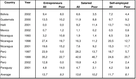
N
Table 2
egarding quantities, and based on the information available for Guatemala, Nicaragua Percentage of individuals with credit, by labor status
Country Year
All Poor All Poor All Poor
Bolivia 2002 9,4 8,0 6,6 3,5 7,2 4,4
Guatemala 2000 13,5 10,2 11,9 8,8 9,7 9,2
Haiti 2001 0,0 0,0 9,2 11,4 13,7 14,3
Mexico 2002 0,7 1,2 1,1 0,2 0,5 0,6
Nicaragua 1993 3,2 10,8 1,9 1,4 6,5 3,9
Nicaragua 1998 27,4 19,7 16,3 11,2 20,5 12,7
Nicaragua 2001 19,6 15,2 7,6 9,2 15,3 11,7
Perú 1997 23,9 0,0 28,2 13,7 18,7 5,7
Perú 1999 35,2 22,7 42,6 46,7 24,6 20,7
Perú 2002 12,8 0,0 19,8 4,3 7,4 2,4
Paraguay 2001 4,8 14,0 4,7 2,1 4,2 3,8
Average 13,7 9,3 13,6 10,2 11,7 8,1
Source: Own elaboration based on SEDLAC.
Entrepreneurs Salaried Self-employed
R
Table 3
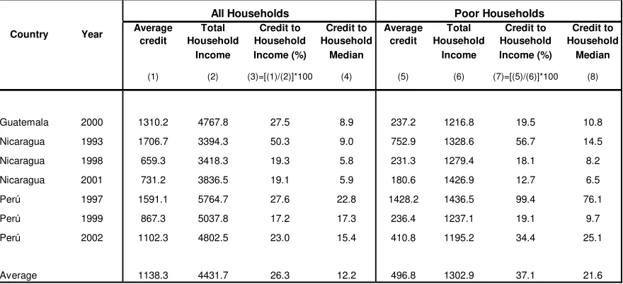
Table 4 we portrait the personal profile of working individuals receiving and not
Amount of Credit to Households
In current U.S. dollars, unless stated otherwise
Country Year Average credit
Total Household
Credit to Household
Credit to Household
Average credit
Total Household
Credit to Household
Credit to Household Income Income (%) Median Income Income (%) Median
(1) (2) (3)=[(1)/(2)]*100 (4) (5) (6) (7)=[(5)/(6)]*100 (8)
Guatemala 2000 1310.2 4767.8 27.5 8.9 237.2 1216.8 19.5 10.8
Nicaragua 1993 1706.7 3394.3 50.3 9.0 752.9 1328.6 56.7 14.5
Nicaragua 1998 659.3 3418.3 19.3 5.8 231.3 1279.4 18.1 8.2
Nicaragua 2001 731.2 3836.5 19.1 5.9 180.6 1426.9 12.7 6.5
Perú 1997 1591.1 5764.7 27.6 22.8 1428.2 1436.5 99.4 76.1
Perú 1999 867.3 5037.8 17.2 17.3 236.4 1237.1 19.1 9.7
Perú 2002 1102.3 4802.5 23.0 15.4 410.8 1195.2 34.4 25.1
Average 1138.3 4431.7 26.3 12.2 496.8 1302.9 37.1 21.6
Poor Households All Households
In
Table 4
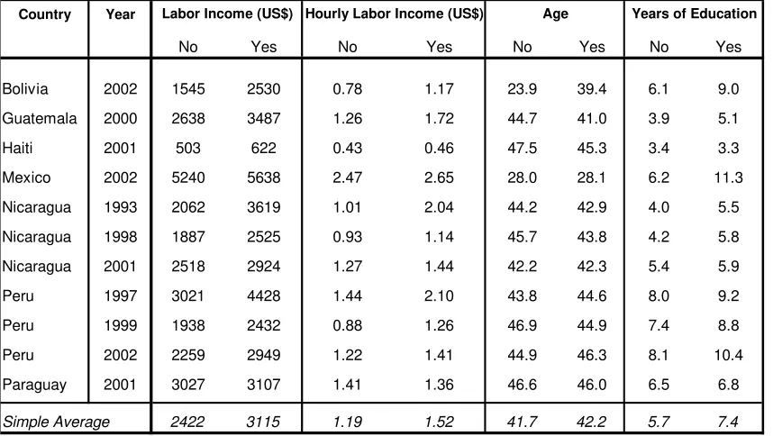
Income and Access to Credit, All Individuals
Country Year
No Yes No Yes No Yes No Yes
Bolivia 2002 1545 2530 0.78 1.17 23.9 39.4 6.1 9.0
Guatemala 2000 2638 3487 1.26 1.72 44.7 41.0 3.9 5.1
Haiti 2001 503 622 0.43 0.46 47.5 45.3 3.4 3.3
Mexico 2002 5240 5638 2.47 2.65 28.0 28.1 6.2 11.3
Nicaragua 1993 2062 3619 1.01 2.04 44.2 42.9 4.0 5.5
Nicaragua 1998 1887 2525 0.93 1.14 45.7 43.8 4.2 5.8
Nicaragua 2001 2518 2924 1.27 1.44 42.2 42.3 5.4 5.9
Peru 1997 3021 4428 1.44 2.10 43.8 44.6 8.0 9.2
Peru 1999 1938 2432 0.88 1.26 46.9 44.9 7.4 8.8
Peru 2002 2259 2949 1.22 1.41 44.9 46.3 8.1 10.4
Paraguay 2001 3027 3107 1.41 1.36 46.6 46.0 6.5 6.8
Simple Average 2422 3115 1.19 1.52 41.7 42.2 5.7 7.4
(*) No (Yes): The individual does not receive (receives) credit. Source: Own elaboration based on SEDLAC.
Hourly Labor Income (US$)
Labor Income (US$) Age Years of Education
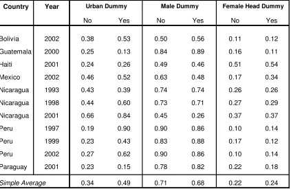
Table 4 (cont.)
Income and Access to Credit, All Individuals (cont.)
Country Year
No Yes No Yes No Yes
Bolivia 2002 0.62 0.81 0.50 0.53 0.15 0.17
Guatemala 2000 0.43 0.47 0.81 0.86 0.19 0.14
Haiti 2001 0.29 0.32 0.50 0.44 0.50 0.56
Mexico 2002 0.75 0.82 0.64 0.65 0.18 0.15
Nicaragua 1993 0.58 0.62 0.71 0.79 0.29 0.21
Nicaragua 1998 0.54 0.71 0.72 0.72 0.28 0.28
Nicaragua 2001 0.76 0.80 0.47 0.31 0.31 0.33
Peru 1997 0.67 0.93 0.83 0.83 0.17 0.17
Peru 1999 0.63 0.80 0.81 0.87 0.19 0.13
Peru 2002 0.63 0.86 0.83 0.80 0.17 0.20
Paraguay 2001 0.56 0.69 0.75 0.75 0.25 0.25
Simple Average 0.59 0.71 0.69 0.69 0.24 0.24
(*) No (Yes): The individual does not receive (receives) credit. Source: Own elaboration based on SEDLAC.
Table 5
Income and Access to Credit, Poor Individuals
Country Year
No Yes No Yes No Yes No Yes
Bolivia 2002 486 641 0.27 0.30 22.3 40.1 4.3 5.4
Guatemala 2000 754 882 0.28 0.39 42.9 40.5 2.0 1.4
Haiti 2001 306 362 0.27 0.32 46.9 45.3 2.7 2.6
Mexico 2002 1289 1177 0.69 0.56 24.7 27.5 3.9 7.1
Nicaragua 1993 872 1120 0.49 0.52 44.3 45.3 2.5 3.4
Nicaragua 1998 737 839 0.38 0.43 45.4 43.3 2.8 4.2
Nicaragua 2001 729 937 0.53 0.59 40.2 41.3 3.6 4.3
Peru 1997 961 1244 0.71 0.77 42.5 44.7 4.5 7.3
Peru 1999 852 799 0.56 0.48 47.1 43.7 3.9 5.2
Peru 2002 751 754 0.41 0.41 42.0 44.5 5.7 5.9
Paraguay 2001 611 639 0.31 0.32 46.6 47.4 3.9 4.1
Simple Average 759 854 0.45 0.46 40.4 42.1 3.6 4.6
(*) No (Yes): The individual does not receive (receives) credit. Source: Own elaboration based on SEDLAC.
Labor Income (US$) Hourly Labor Income (US$) Age Years of Education
Table 5 (cont.)
Income and Access to Credit, Poor Individuals (cont.)
Country Year
No Yes No Yes No Yes
Bolivia 2002 0.38 0.53 0.50 0.56 0.11 0.12
Guatemala 2000 0.25 0.13 0.84 0.89 0.16 0.11
Haiti 2001 0.24 0.26 0.49 0.46 0.51 0.54
Mexico 2002 0.46 0.52 0.63 0.48 0.17 0.34
Nicaragua 1993 0.43 0.39 0.74 0.74 0.26 0.26
Nicaragua 1998 0.44 0.60 0.73 0.71 0.27 0.29
Nicaragua 2001 0.66 0.84 0.45 0.26 0.37 0.37
Peru 1997 0.19 0.90 0.90 0.86 0.10 0.14
Peru 1999 0.23 0.43 0.83 0.88 0.17 0.12
Peru 2002 0.27 0.62 0.90 0.86 0.10 0.14
Paraguay 2001 0.23 0.15 0.78 0.82 0.22 0.18
Simple Average 0.34 0.49 0.71 0.68 0.22 0.24
(*) No (Yes): The individual does not receive (receives) credit. Source: Own elaboration based on SEDLAC.
As for schooling, Tables 6 and 7 reveal that children from credit-receiving households display, on average, higher levels of primary and secondary school attendance. Furthermore, these households typically have higher per capita income, live in a city and have more educated parents.
Table 6
Primary School Attendance and Access to Credit
No Yes No Yes No Yes No Yes No Yes Bolivia 2002 0.93 0.97 482 795 0.56 0.77 6.48 8.50 5.53 7.53 Guatemala 2000 0.75 0.84 729 913 0.34 0.31 3.30 3.68 2.77 3.20 Haiti 2001 0.77 0.83 198 181 0.25 0.30 3.08 3.42 3.13 3.41 Mexico 2002 0.97 0.97 1379 1774 0.70 0.71 6.75 7.47 6.35 7.24 Nicaragua 1993 0.96 0.92 485 901 0.53 0.66 3.51 5.39 3.50 4.78 Nicaragua 1998 0.82 0.94 489 642 0.50 0.65 3.88 5.30 3.69 4.89 Nicaragua 2001 0.91 0.95 622 901 0.68 0.79 4.30 5.19 4.27 4.75 Peru 1997 0.95 0.98 827 1102 0.54 0.91 7.22 9.28 6.07 7.89 Peru 1999 0.97 0.96 586 749 0.52 0.71 7.19 7.78 6.15 6.46 Peru 2002 0.97 1.00 727 1186 0.57 0.78 7.84 9.95 6.65 8.65 Paraguay 2001 0.94 0.98 764 1006 0.46 0.58 6.00 6.26 5.47 5.73 Simple Average 0.90 0.94 663 923 0.51 0.65 5.41 6.57 4.87 5.87
(*) No (Yes): The individual does not receive (receives) credit. Source: Own elaboration based on SEDLAC.
Years of Education, Household Adults Per Capita
Household Income (current US$)
Urban Dummy Years of Education, Household Head Country Year School Attendance
[image:14.595.89.511.496.683.2]Dummy
Table 7
Secondary School Attendance and Access to Credit
No Yes No Yes No Yes No Yes No Yes Bolivia 2002 0.82 0.89 562 820 0.60 0.75 6.61 8.20 5.80 7.31 Guatemala 2000 0.51 0.57 823 804 0.38 0.33 3.11 3.16 2.79 2.72 Haiti 2001 0.77 0.80 213 201 0.33 0.35 3.35 3.23 3.52 3.47 Mexico 2002 0.71 0.89 1619 2145 0.72 0.77 6.22 7.62 6.06 7.63 Nicaragua 1993 0.70 0.64 522 933 0.55 0.55 3.29 5.23 3.39 5.02 Nicaragua 1998 0.58 0.71 539 1092 0.51 0.70 3.67 5.39 3.67 5.17 Nicaragua 2001 0.75 0.76 896 906 0.71 0.81 4.57 6.20 4.61 5.58 Peru 1997 0.78 0.85 1283 1086 0.65 0.89 7.53 7.79 6.27 6.71 Peru 1999 0.81 0.92 771 946 0.57 0.69 7.34 8.25 6.17 6.93 Peru 2002 0.81 0.92 720 1250 0.57 0.84 7.23 10.13 5.95 8.91 Paraguay 2001 0.72 0.80 922 1087 0.51 0.59 6.00 6.39 5.48 5.86 Simple Average 0.72 0.80 806 1024 0.55 0.66 5.36 6.51 4.88 5.94
(*) No (Yes): The individual does not receive (receives) credit. Source: Own elaboration based on SEDLAC.
Country Year School Attendance Dummy
Per Capita Household Income
(current US$)
Urban Dummy Years of Education, Household Head
3. Econometric Analysis
In what follows we discuss our empirical findings on the effect of credit on labor income (section 3.1) and primary and secondary schooling decisions (section 3.2) of poor households. Summarizing our subsequent remarks, we find that credit (proxied by a dummy with value one if the worker got a loan over the last 12 months) boosts labor income in a statistically and economically significant fashion in three out of the seven household surveys under study. In two out of four surveys with loan quantity data available, we observe an equally significant impact. As for education, the access to credit improves primary (secondary) school attainment in five (three) out of eleven household surveys, with the effect running through the ability to get credit and independently of the amount obtained.
3.1 Income Regressions
Our first econometric exercise centers on the impact of credit on the income of poor households. The dependent variable is the natural logarithm of the hourly labor income of the household head. We restrict the analysis to poor workers, as this is our population of interest and because, from an econometric standpoint, endogeneity caveats are largely mitigated when other income recipients are dropped from the sample. Since we are interested in assessing whether the access to credit raises labor income by allocating borrowed money to profitable productive projects, we exclude observations with zero income and those for salaried individuals: in the first case, because it is evident that the individual, even having received credit, did not allocate it to any productive project;4 in the second case, because employed workers earning a salary do not undertake, by
definition, investment projects by themselves.5 Guided by this criterion, we also
discarded the Mexico and Peru surveys because they explicitly state that the loan is not to be used for investment purposes. We perform two sets of regressions, one including just a dummy variable indicating whether the individual had any credit, and the other including the amount received. Besides the credit variables just described, we will control for schooling, age, gender, and residence (urban or rural).
4 Alternatively, he or she might have allocated it to a project with nil gross revenue, a situation quite
unlikely.
5 Ideally, we would like survey respondents to clearly state whether the loan was used for consumption or
Table 8
Credit Dummy and Labor Income: OLS Baseline Regressions
Dependent Variable: Bolivia Guatemala Haiti Nicaragua Nicaragua Nicaragua Paraguay
Ln(Hourly Labor Income) 2002 2000 2001 1993 1998 2001 2001
=1 if received a loan 0.274* 1.247*** 0.197** 0.325 0.041 0.07 0.155
[0.164] [0.287] [0.081] [0.230] [0.123] [0.180] [0.151]
=1 if s(he) is self-employed -0.291* 0.804** -0.845 -0.596 -0.451*** 0.095 -0.673***
[0.149] [0.334] [0.555] [0.548] [0.104] [0.197] [0.089]
=1 if primary school complete 0.401** 0.044 0.22 0.311* -0.011 0.161 0.184*
[0.164] [0.370] [0.231] [0.175] [0.125] [0.189] [0.101]
=1 if secondary school incomplete 0.432*** -0.228 -0.155 0.307* 0.243 0.275 0.29
[0.117] [0.423] [0.185] [0.174] [0.164] [0.297] [0.186]
=1 if secondary school complete 0.298* -0.165 -0.930*** 0.940** 0.385** -0.249 -0.034
[0.178] [0.910] [0.102] [0.461] [0.181] [0.656] [0.227]
=1 if superior school incomplete -0.094 1.656*** -0.809 -2.671*** 0.58 0 0.135
[0.389] [0.373] [0.569] [0.253] [0.554] [0.000] [0.437]
=1 if superior school complete 0.558** 0.810** 2.837* 0.772 -0.158 1.06 0.054
[0.280] [0.322] [1.490] [0.482] [0.113] [0.908] [0.108]
Age 0.065*** 0.157** 0.029 0.063** -0.028 0.083* 0.046**
[0.021] [0.065] [0.018] [0.028] [0.024] [0.049] [0.021]
Age squared -0.001*** -0.002** -0.000** -0.001** 0 -0.001* -0.001**
[0.000] [0.001] [0.000] [0.000] [0.000] [0.001] [0.000]
=1 if male 0.227** 0.376 0.162*** -0.221 -0.314*** 0.018 -0.260*
[0.101] [0.468] [0.058] [0.163] [0.111] [0.151] [0.138]
=1 if urban 0.847*** 0 -0.578*** 0.332** 0.248*** 0.222 1.285*
[0.085] [0.000] [0.078] [0.130] [0.094] [0.139] [0.692]
Constant -4.250*** -6.572*** -1.420** -1.411* 0.29 -3.055*** -3.156***
[0.464] [1.467] [0.680] [0.759] [0.524] [1.085] [0.829]
Observations 1369 226 2294 853 821 228 1033
R-squared 0.23 0.18 0.09 0.21 0.13 0.08 0.17
Sigma 1.15 1.27 1.24 1.1 1.05 0.84 0.94
Robust standard errors in brackets
Table 9
e go a step further in Tables 10 and 11 by entering the amount of credit instead of the Credit Dummy and Labor Income: OLS Additional Regressions
Dependent Variable: Bolivia Guatemala Haiti Nicaragua Nicaragua Nicaragua Paraguay
Ln(Hourly Labor Income) 2002 2000 2001 1993 1998 2001 2001
=1 if received a loan 0.273* 1.164*** 0.225*** 0.25 0.061 0.078 0.178 [0.162] [0.280] [0.084] [0.235] [0.128] [0.176] [0.147] =1 if s(he) is self-employed -0.293** 0.618** -0.81 -0.692 -0.447*** 0.071 -0.648***
[0.149] [0.305] [0.587] [0.545] [0.104] [0.241] [0.086] =1 if s(he) has at least 7 years of education 0.370*** 0.312 0.121 0.445* 0.326*** 0.362 0.066
[0.095] [0.373] [0.089] [0.232] [0.110] [0.378] [0.188]
Age 0.064*** 0.179*** 0.028 0.066** -0.026 0.085* 0.043**
[0.020] [0.069] [0.018] [0.028] [0.024] [0.050] [0.022] Age squared -0.001*** -0.002*** -0.000** -0.001*** 0 -0.001* -0.001**
[0.000] [0.001] [0.000] [0.000] [0.000] [0.001] [0.000]
=1 if male 0.221** 0.375 0.152*** -0.216 -0.298*** 0.025 -0.252*
[0.101] [0.469] [0.059] [0.171] [0.111] [0.147] [0.140]
=1 if urban 0.836*** 0 -0.634*** 0.354*** 0.253*** 0.223 1.351*
[0.085] [0.000] [0.079] [0.129] [0.090] [0.140] [0.705] Constant -4.218*** -6.915*** -1.451** -1.308* 0.281 -3.013*** -3.065***
[0.462] [1.481] [0.712] [0.777] [0.528] [1.105] [0.831]
Observations 1370 233 2250 853 821 228 1033
R-squared 0.23 0.15 0.08 0.2 0.13 0.07 0.17
Sigma 1.15 1.28 1.24 1.11 1.05 0.85 0.94
Notes:
Robust standard errors in brackets
* significant at 10%; ** significant at 5%; *** significant at 1% The regressions include unreported regional dummies.
W
Table 10
Credit Amount and Labor Income: OLS Baseline Regressions
Dependent Variable: Guatemala Nicaragua Nicaragua Nicaragua
Ln(Hourly Labor Income) 2000 1993 1998 2001
Loan amount 0.002* 0 0 0.001
[0.001] [0.000] [0.000] [0.001]
=1 if s(he) is self-employed 0.876** -0.624 -0.440*** 0.092
[0.360] [0.523] [0.105] [0.194]
=1 if primary school complete -0.091 0.304* -0.024 0.152
[0.368] [0.175] [0.125] [0.191]
=1 if secondary school incomplete -0.438 0.320* 0.244 0.276
[0.432] [0.174] [0.169] [0.297]
=1 if secondary school complete -0.323 0.931** 0.393** -0.427
[0.901] [0.458] [0.181] [0.522]
=1 if superior school incomplete 1.628*** 0 0.589 0
[0.390] [0.000] [0.554] [0.000]
=1 if superior school complete 0.522 0.884 -0.147 1.059
[0.373] [0.571] [0.112] [0.905]
Age 0.158** 0.064** -0.028 0.081*
[0.068] [0.028] [0.024] [0.049]
Age squared -0.002** -0.001** 0 -0.001*
[0.001] [0.000] [0.000] [0.001]
=1 if male 0.396 -0.224 -0.319*** 0.026
[0.484] [0.163] [0.111] [0.151]
=1 if urban 0 0.337*** 0.237** 0.221
[0.000] [0.130] [0.093] [0.139]
Constant -6.360*** -1.404* 0.3 -3.014***
[1.522] [0.741] [0.518] [1.083]
Observations 226 851 823 228
R-squared 0.14 0.2 0.13 0.09
Sigma 1.3 1.1 1.05 0.84
Notes:
Robust standard errors in brackets
Table 11
s announced in the Introduction, we explored in unreported exercises the role of
ne controversial issue is whether the significance of the credit coefficient is picking up Credit Amount and Labor Income: OLS Additional Regressions
Dependent Variable: Guatemala Nicaragua Nicaragua Nicaragua
Ln(Hourly Labor Income) 2000 1993 1998 2001
Loan amount 0.002* 0 0.001 0.001
[0.001] [0.000] [0.000] [0.000] =1 if s(he) is self-employed 0.706** -0.695 -0.436*** 0.063
[0.331] [0.528] [0.104] [0.248] =1 if s(he) has at least 7 years of education 0.136 0.527** 0.333*** 0.254
[0.395] [0.226] [0.110] [0.266]
Age 0.187*** 0.066** -0.026 0.086*
[0.071] [0.028] [0.024] [0.050]
Age squared -0.002*** -0.001*** 0 -0.001*
[0.001] [0.000] [0.000] [0.001]
=1 if male 0.389 -0.208 -0.304*** 0.038
[0.483] [0.171] [0.111] [0.150]
=1 if urban 0 0.376*** 0.243*** 0.221
[0.000] [0.128] [0.090] [0.137]
Constant -6.960*** -1.331* 0.291 -3.017***
[1.564] [0.764] [0.527] [1.090]
Observations 233 851 823 228
R-squared 0.11 0.2 0.13 0.07
Sigma 1.3 1.11 1.05 0.85
Notes:
Robust standard errors in brackets
* significant at 10%; ** significant at 5%; *** significant at 1% The regressions include unreported regional dummies.
A
gender. In particular, we wanted to assess whether female household heads allocate loans more efficiently than male heads. To this end, in addition to the credit variables included in the previous regressiones, we included the interaction of those variables with a dummy taking the value one for households with a female head, and zero otherwise. However, in no case did we find a significant gender effect.
O
vary substantially between two given poor borrowers in spite of narrow income differences. Second, commercial banks are usually not prone to extend credit to members of these income groups, which mostly rely on public or publicly sponsored microcredit programs where credit allocation is not necessarily governed by the borrower´s financial strength –it may even be the case that some programs target extremely poor households as a poverty reduction mechanism.6
Another concern has to do with the potential presence of selection bias. Let us recall
.2 Education Regressions
ns to estimate the probability of attending primary and
that we are primarily interested in testing how the access to credit affects labor income, and that is why we excluded from our estimations all unemployed household headsbecause, by definition, the gross return on their loans –in case they got one- is zero. Nevertheless, in order to make sure that our results are not driven by selection bias, we re-run our baseline regressions from Table 8 and 10 but adding to the sample the unemployed household heads and using the two-step Heckman technique. The estimated coefficients did not change much: relative to the credit dummy estimates of Table 8, the coefficients for Bolivia, Guatemala and Haiti fell by just 3.4%, 0.2% and 3.1%, respectively, while no variation was found in the credit amount regressions. The regression output is not reported, but it is available upon request.
3
e employ probit regressio W
secondary school for children of 6 to 12 and 13 to 17 years old, respectively. Our variable of interest is whether the household received a loan during the last 12 months (and alternatively how much it received as a ratio of total household income). In order to take into account other schooling determinants, we include several controls. Invoking the arguments of the last paragraph, we expect that the higher the per capita household income, the higher the attendance. Households from rural areas should also exhibit lower education levels, owing to likely higher distance to schools, more child labor and higher income risk. The preference for education may be encouraged by more educated
6 An alternative procedure is to instrumentalize credit. In unreported regressions (available upon request),
household heads, as measured by his or her years of education. Child age and gender are also included, although the expected sign is ambiguous. Regarding age, it might be the case that older children are perceived to have a larger labor opportunity cost, but on the other hand it is possible that younger children stay at home beyond the age of 6.7 As for gender, it is an empirical question whether boys or girls are more likely to prematurely enter the labor market. A priori, boys may start working before girls, but girls are sometimes required to take care of household chores, including babysitting for younger siblings. An important issue is the role of female household heads in education decisions. In line with our previous discussion, we expect the probability of staying at school to be higher in households receiving credit and with a female head.8
Next we report the marginal probabilities of staying in primary school obtained from the
probit regressions. Since we do not suspect any endogeneity bias contaminating the results, we first run regressions for the whole sample. In Table 12A and 12B we present the cases where the credit dummy was and was not significantly positive, respectively. Having access to credit significantly improves the probability of staying at school in Bolivia (2002), Guatemala (2000), Haiti (2001), Mexico (2002), and Nicaragua (1998 and 2001). The rise in probability ranges from 2.3% in Bolivia to 9.2% in Nicaragua (1998). The additional controls that deliver positive and significant loadings in most (but, as earlier, not in all) cases are Age, Per capita household income, the Urban dummy, and Years of education of the household head. The presence of a female household head shows the expected positive sign at acceptable significance levels in four out of the eleven regressions.
7 It must be borne in mind that the mandatory primary school status in most countries is not always
properly enforced.
8 Marchionni and Sosa Escudero (1999), however, find for Argentina that secondary schooling is
Table 12A
Credit Dummy and Primary Education: Marginal Probabilities All Households
Dependent Variable: Probability of Bolivia Guatemala Haiti Mexico Nicaragua Nicaragua
Staying in Primary School 2002 2000 2001 2002 1998 2001
=1 if Household Received a Loan 0.023*** 0.063*** 0.042*** 0.017*** 0.092*** 0.031** [0.008] [0.013] [0.015] [0.006] [0.013] [0.012]
[image:23.595.92.524.481.735.2]Age 0.014*** 0.056*** 0.028*** -0,001 0.017*** 0.011***
[0.001] [0.002] [0.003] [0.001] [0.003] [0.003]
=1 if Male 0,005 0.047*** -0,009 -0,002 -0.049*** -0,013
[0.006] [0.010] [0.011] [0.003] [0.011] [0.011]
Per Capita Household Income 0 0.000*** 0.000*** 0 0.000*** 0.000***
[0.000] [0.000] [0.000] [0.000] [0.000] [0.000]
=1 if Urban 0.020*** 0.061*** 0.058*** -0,003 0.112*** 0.034***
[0.007] [0.010] [0.015] [0.003] [0.012] [0.013] Years of Education of Household Head 0.006*** 0.030*** 0.023*** 0.003*** 0.023*** 0.006***
[0.001] [0.002] [0.002] [0.000] [0.002] [0.002]
=1 if Household Head is Female 0,002 0.030** 0.034*** -0,001 0.040*** 0,008
[0.009] [0.013] [0.012] [0.004] [0.012] [0.011]
Observations 4656 7299 5032 11084 4477 1744
Chi2 202,04 1149,17 423,04 119,72 586,93 107,55
Standard errors in brackets
* significant at 10%; ** significant at 5%; *** significant at 1%
Table 12B
Credit Dummy and Primary Education: Marginal Probabilities (Cont.) All Households
Dependent Variable: Probability of Nicaragua Peru Peru Peru Paraguay
Staying in Primary School 1993 1997 1999 2002 2001
=1 if Household Received a Loan -0,024 -0,014 -0,009 0,006 0,011 [0.019] [0.019] [0.013] [0.004] [0.009]
Age -0.008*** 0.009*** 0.006** 0.003*** 0.009***
[0.001] [0.003] [0.003] [0.001] [0.001]
=1 if Male -0,007 0,006 0,009 -0,002 -0,006
[0.005] [0.011] [0.011] [0.003] [0.004]
Per Capita Household Income 0 0 0 0.000** 0.000**
[0.000] [0.000] [0.000] [0.000] [0.000]
=1 if Urban 0.021*** 0,022 0.037** 0,007 0.015***
[0.007] [0.017] [0.017] [0.005] [0.005] Years of Education of Household Head 0.004*** 0,002 -0,001 0.001* 0.008***
[0.001] [0.001] [0.002] [0.000] [0.001] =1 if Household Head is Female -0,01 -0,051 0,001 0 0.009** [0.007] [0.036] [0.020] [0.005] [0.005]
Observations 3913 734 557 1777 6738
Chi2 108,64 29,07 15,8 59,36 321,4
Standard errors in brackets
We restrict the sample to poor households in Tables 13A and 13B. The positive and significant coefficients appear in Table 13A, which encompasses the cases of Bolivia (2002), Guatemala (2000), Haiti (2001), Nicaragua (2001) and Paraguay (2001). The marginal effect on the probability goes from a minimum of 4.3% in Paraguay to 10.6% in Nicaragua (1998). In these cases, once again, Age, Per capita household income, Urban residence and Years of education of the household head display, for the most part, positive and significant signs, while Female head does it in two of the five regressions.9 The regressions in Table 13B show non significant credit effects (with the odd exception of a negative one in Nicaragua (1993)) and a wider variation in the sign and significance of the control set.
9 We repeated the gender test run in the income regressions by adding the interaction between the credit
Table 13A
Credit Dummy and Primary Education: Marginal Probabilities Poor Households
Dependent Variable: Probability of Bolivia Guatemala Haiti Nicaragua Paraguay
Staying in Primary School 2002 2000 2001 1998 2001
=1 if Household Received a Loan 0.045*** 0.102*** 0.042** 0.106*** 0.043*** [0.013] [0.029] [0.016] [0.023] [0.015]
Age 0.019*** 0.075*** 0.031*** 0.023*** 0.017***
[0.002] [0.005] [0.003] [0.004] [0.002]
=1 if Male 0.002 0.077*** -0.011 -0.066*** -0.006
[0.010] [0.019] [0.012] [0.016] [0.010] Per Capita Household Income 0 0.000*** 0.000*** 0.000*** 0.000***
[0.000] [0.000] [0.000] [0.000] [0.000]
=1 if Urban 0.005 0.033 0.058*** 0.112*** 0.020*
[0.012] [0.023] [0.017] [0.017] [0.011] Years of Education of Household Head 0.008*** 0.038*** 0.024*** 0.024*** 0.016***
[0.002] [0.004] [0.002] [0.003] [0.002] =1 if Household Head is Female -0.004 0.006 0.035*** 0.052*** 0.005
[0.016] [0.029] [0.013] [0.019] [0.012]
Observations 2524 2595 4522 2893 2428
Chi2 114.1 356.23 349.1 296.27 140.39
Standard errors in brackets
Table 13B
e explore the relevance of the amount of credit received –as opposed to whether the ** Credit Dummy and Primary Education: Marginal Probabilities (Cont.)
Poor Households
Dependent Variable: Probability of Mexico Nicaragua Nicaragua Peru Peru Peru
Staying in Primary School 2002 1993 2001 1997 1999 2002
=1 if Household Received a Loan -0.083** 0,018 -0,039 0,023 -0,007
[0.040] [0.038] [0.102] [0.030] [0.034]
Age -0,001 -0.011*** 0.021*** 0.027*** 0,006 0.010***
[0.001] [0.002] [0.006] [0.008] [0.008] [0.003]
=1 if Male -0,005 -0,002 -0,037 0,002 0,034 -0,004
[0.006] [0.008] [0.024] [0.028] [0.034] [0.010]
Per Capita Household Income 0.000** 0 0 0 0 0.000
[0.000] [0.000] [0.000] [0.000] [0.000] [0.000]
=1 if Urban -0.018*** 0.029*** 0.078*** 0,037 0.032***
[0.007] [0.010] [0.027] [0.033] [0.010]
Years of Education of Household Head 0.006*** 0.004*** 0.014*** 0,003 -0,006 0 [0.001] [0.002] [0.004] [0.004] [0.005] [0.001]
=1 if Household Head is Female 0,003 -0.019* 0,012 -0,074 0
[0.008] [0.011] [0.025] [0.123] [0.026]
Observations 3907 2538 820 242 177 720
Chi2 51,09 69,17 41,29 17,07 5,47 32,42
Standard errors in brackets
* significant at 10%; ** significant at 5%; *** significant at 1%
W
Table 14
able 15
e repeat the previous experiments looking now at the decision to stay in secondary
Bolivia, Guatemala, Haiti, Mexico, Nicaragua (1998), Peru (1999), and Paraguay. The Credit Amount and Primary Education: Marginal Probabilities
All Households
Dependent Variable: Probability of Guatemala Nicaragua Nicaragua Nicaragua Peru Peru Peru Staying in Primary School 2000 2001 1993 1998 1997 1999 2002
Credit Amount 0.000*** 0.000** 0 0 0 0 0
[0.000] [0.000] [0.000] [0.000] [0.000] [0.000] [0.000]
Age 0.055*** 0.015*** -0.008*** 0.017*** 0.006*** 0.004*** 0.004*** [0.002] [0.002] [0.001] [0.003] [0.001] [0.001] [0.001]
[image:27.595.87.528.437.635.2]=1 if Male 0.046*** -0.014 -0.007 -0.050*** 0.008 0.011** 0
[0.010] [0.009] [0.005] [0.011] [0.005] [0.005] [0.002]
Per Capita Household Income 0.000*** 0.000*** 0 0.000*** 0.000*** 0.000** 0.000*** [0.000] [0.000] [0.000] [0.000] [0.000] [0.000] [0.000]
=1 if Urban 0.057*** 0.084*** 0.020*** 0.116*** 0.014** 0.01 0.013*** [0.010] [0.010] [0.007] [0.012] [0.006] [0.006] [0.003]
Years of Education of Household Head 0.030*** 0.016*** 0.004*** 0.024*** 0.005*** 0.003*** 0.002*** [0.002] [0.002] [0.001] [0.002] [0.001] [0.001] [0.000]
=1 if Household Head is Female 0.028** 0.027*** -0.01 0.040*** 0.004 0.007 0.001 [0.013] [0.010] [0.007] [0.013] [0.007] [0.006] [0.003] Observations 7300 4567 3918 4484 5506 3044 14391 Chi2 1147.29 487.55 107.07 553.88 204.77 83.84 326.11
Standard errors in brackets
* significant at 10%; ** significant at 5%; *** significant at 1%
T
Credit Amount and Primary Education: Marginal Probabilities
Poor Households
Dependent Variable: Probability of Guatemala Nicaragua Nicaragua Nicaragua Peru Peru Peru Staying in Primary School 2000 1998 1993 2001 1997 1999 2002
Credit Amount 0.000* 0.000** 0 0 0 0 0
[0.000] [0.000] [0.000] [0.000] [0.000] [0.000] [0.000]
Age 0.074*** 0.023*** -0.011*** 0.022*** 0.014*** 0.008*** 0.008*** [0.005] [0.004] [0.002] [0.004] [0.003] [0.003] [0.001]
=1 if Male 0.076*** -0.067*** -0.002 -0.019 0.015 0.012 0.002
[0.019] [0.016] [0.008] [0.015] [0.011] [0.011] [0.004]
Per Capita Household Income 0.000*** 0.000*** 0 0.000** 0.000* 0 0.000*** [0.000] [0.000] [0.000] [0.000] [0.000] [0.000] [0.000]
=1 if Urban 0.031 0.115*** 0.030*** 0.118*** 0.013 0.021* 0.020***
[0.023] [0.017] [0.010] [0.016] [0.014] [0.012] [0.005]
Years of Education of Household Head 0.037*** 0.025*** 0.004** 0.026*** 0.009*** 0.006*** 0.004*** [0.004] [0.003] [0.002] [0.003] [0.002] [0.002] [0.001]
=1 if Household Head is Female 0.005 0.050*** -0.018* 0.041** 0.011 0.001 0.015*** [0.029] [0.019] [0.011] [0.017] [0.016] [0.016] [0.005] Observations 2595 2898 2539 2754 2627 1370 6872 Chi2 348.94 282.58 62.09 238.73 69.64 27.46 184.74
Standard errors in brackets
* significant at 10%; ** significant at 5%; *** significant at 1%
W
marginal effect reaches a minimum of 4.8% for Haiti and a maximum of 10.6% for Mexico. Among the controls, in all cases, Years of education of the household head and the Urban dummy appear as the most robust ones, along with Age, which now enters negatively (indicating that older teenagers drop out from school to start working). The gender of the household head does not seem to be influential on the secondary schooling decision.
For poor households, credit has a significantly positive impact in Haiti, Mexico, and eru (1999), as shown in Tables 17A and 17B, with marginal probabilities of 5.7%, P
Table 16A
able 16B
Credit Dummy and Secondary Education: Marginal Probabilities
All Households
Dependent Variable: Probability of Bolivia Guatemala Haiti Mexico Nicaragua Peru Paraguay
Staying in Secondary School 2002 2000 2001 2000 1998 1999 2001
[image:29.595.88.525.421.674.2]=1 if Household Received a Loan 0.049*** 0.086*** 0.048** 0.106*** 0.055* 0.077** 0.074*** [0.015] [0.025] [0.019] [0.030] [0.029] [0.038] [0.026] Age -0.047*** -0.112*** -0.028*** -0.121*** -0.103*** -0.067*** -0.076***
[0.004] [0.006] [0.005] [0.004] [0.007] [0.013] [0.004]
=1 if Male 0.029** 0.096*** -0,001 0,008 -0.061*** -0,024 0,013
[0.012] [0.016] [0.015] [0.010] [0.020] [0.038] [0.012]
Per Capita Household Income 0 0.000*** 0 0.000*** 0 0 0.000***
[0.000] [0.000] [0.000] [0.000] [0.000] [0.000] [0.000] =1 if Urban 0.131*** 0.249*** 0.069*** 0.029** 0.255*** 0.099** 0.127***
[0.014] [0.017] [0.018] [0.012] [0.021] [0.049] [0.014] Years of Education of Household Head 0.017*** 0.040*** 0.015*** 0.028*** 0.046*** 0.009* 0.030***
[0.002] [0.003] [0.002] [0.001] [0.003] [0.005] [0.002] =1 if Household Head is Female 0,02 0,028 0,019 -0,016 0,015 -0,043 0,015
[0.015] [0.022] [0.016] [0.014] [0.023] [0.060] [0.014]
Observations 2956 4337 2898 7452 2886 311 4384
Chi2 461,79 1175,37 127,39 1691,92 800,85 49,08 859,38
Standard errors in brackets
* significant at 10%; ** significant at 5%; *** significant at 1%
T
Credit Dummy and Secondary Education: Marginal Probabilities (Cont.)
All Households
Dependent Variable: Probability of Nicaragua Nicaragua Peru Peru
Staying in Secondary School 1993 2001 1997 2002
=1 if Household Received a Loan -0,021 -0,026 0,039 0,043 [0.053] [0.036] [0.035] [0.026]
Age -0.098*** -0.086*** -0.078*** -0.062***
[0.007] [0.010] [0.012] [0.007]
=1 if Male -0,026 -0.062** 0,002 0.080***
[0.019] [0.026] [0.032] [0.020]
Per Capita Household Income 0 0.000* 0 0
[0.000] [0.000] [0.000] [0.000]
=1 if Urban 0.261*** 0.109*** 0,032 0.061**
[0.022] [0.031] [0.041] [0.024] Years of Education of Household Head 0.020*** 0.023*** 0.017*** 0.010***
[0.003] [0.004] [0.004] [0.003] =1 if Household Head is Female -0,024 0.051* -0,024 -0,02
[0.021] [0.027] [0.045] [0.030]
Observations 2528 1140 482 1100
Chi2 512,91 167,8 84,27 133,39
Standard errors in brackets
Table 17A
able 17B
y and Secondary Education: Marginal Probabilities
Poor Households
Dependent Variable: Probability of Haiti Mexico Peru
Staying in Secondary School 2001 2000 1999
[image:30.595.90.526.517.680.2]=1 if Household Received a Loan 0.057*** 0.182*** 0.148** [0.021] [0.061] [0.066]
Age -0.029*** -0.155*** -0.050**
[0.006] [0.008] [0.025]
=1 if Male 0,004 0.060*** 0,046
[0.017] [0.021] [0.075]
Per Capita Household Income 0.000*** 0 -0,001
[0.000] [0.000] [0.000]
=1 if Urban 0.077*** 0.048** 0.242***
[0.020] [0.023] [0.061] Years of Education of Household Head 0.015*** 0.029*** 0,002
[0.003] [0.004] [0.014] =1 if Household Head is Female 0,013 -0,014 -0,228 [0.017] [0.029] [0.196]
Observations 2536 2223 102
Chi2 106 478,99 19,38
Standard errors in brackets
* significant at 10%; ** significant at 5%; *** significant at 1% Credit Dumm
T
Credit Dummy and S
Poor Households
econdary Education: Marginal Probabilities (Cont.)
ependent Variable: Probability of Bolivia Guatemala Nicaragua Nicaragua Nicaragua Peru Peru Paragua
D y
Staying in Secondary School 2002 2000 1993 1998 2001 1997 2002 2001 =1 if Household Received a Loan 0,049 0,07 -0,06 0,06 -0,062 -0.517** 0,083 0,098 [0.032] [0.052] [0.083] [0.041] [0.072] [0.205] [0.097] [0.072] Age -0.062*** -0.105*** -0.120*** -0.090*** -0.084*** -0.137*** -0.064*** -0.108***
[0.007] [0.011] [0.009] [0.009] [0.016] [0.030] [0.014] [0.011] =1 if Male 0.048** 0.111*** -0,029 -0.049* -0,052 0,082 0.144*** 0,027
[0.021] [0.030] [0.026] [0.026] [0.044] [0.084] [0.043] [0.029] Per Capita Household Income 0 0.000* 0.000** 0.000** 0 0.001** 0 0.001***
[0.000] [0.000] [0.000] [0.000] [0.000] [0.000] [0.000] [0.000] =1 if Urban 0.161*** 0.153*** 0.259*** 0.202*** 0.108** 0,065 0,055 0.082** [0.021] [0.036] [0.027] [0.027] [0.050] [0.112] [0.046] [0.035] Years of Education of Household Head 0.026*** 0.039*** 0.017*** 0.044*** 0.029*** 0.030** 0,01 0.034***
[0.003] [0.008] [0.005] [0.005] [0.008] [0.014] [0.007] [0.006] =1 if Household Head is Female 0,008 0,01 -0,03 0,026 0,064 0,078 -0,028 -0,023 [0.030] [0.043] [0.029] [0.029] [0.046] [0.119] [0.074] [0.038] Observations 1369 1165 1568 1715 469 123 377 1267 Chi2 241,54 169,08 314,22 344,09 55,6 36,52 37,81 186,21
Standard errors in brackets
The effects of the amount of credit appear in Table 18 (all households) and Table 19 (poor households). In neither of these cases do we observe an economically significant coefficient.
Table 18
Credit Amount and Secondary Education: Marginal Probabilities
All Households
Dependent Variable: Probability of Guatemala Nicaragua Nicaragua Nicaragua Peru Peru Peru
Staying in Secondary School 2000 2001 1993 1998 1997 1999 2002
Credit Amount 0 0 0 0 0 0.000* 0
[0.000] [0.000] [0.000] [0.000] [0.000] [0.000] [0.000]
Age -0.112*** -0.098*** -0.103*** -0.113*** -0.081*** -0.082*** -0.077***
[0.006] [0.007] [0.007] [0.007] [0.005] [0.006] [0.002]
1 if Male 0.096*** -0.025 -0.062*** -0.082*** 0.007 -0.011 0.038*** ]
*
[image:31.595.90.527.521.730.2]*
[0.017] [0.022] [0.021] [0.020] [0.016] [0.020] [0.009]
of Household Head 0.041*** 0.020*** 0.047*** 0.031*** 0.019*** 0.014*** 0.009***
[0.003] [0.003] [0.003] [0.003] [0.002] [0.002] [0.001]
f Household Head is Female 0.025 -0.024 0.015 0.066*** 0.046*** -0.006 0.013
[0.022] [0.021] [0.023] [0.021] [0.016] [0.023] [0.009]
Observations 4337 2529 2891 2855 3549 2063 9487
Chi2 1163.8 513.25 799.42 689.18 538.6 325.46 1336.35
Standard errors in brackets
* significant at 10%; ** significant at 5%; *** significant at 1% =
[0.016] [0.019] [0.020] [0.019] [0.013] [0.017] [0.007
Per Capita Household Income 0.000*** 0 0 0.000*** 0 0 0.000**
[0.000] [0.000] [0.000] [0.000] [0.000] [0.000] [0.000]
=1 if Urban 0.246*** 0.261*** 0.258*** 0.198*** 0.085*** 0.112*** 0.080**
Years of Education =1 i
Table 19
Credit Amount and Secondary Education: Marginal Probabilities
Poor Households
Dependent Variable: Probability of Guatemala Nicaragua Nicaragua Nicaragua Peru Peru Peru
Staying in Secondary School 2000 2001 1993 1998 1997 1999 2002
Credit Amount 0 0 0 0 -0.000* 0.001 0
[0.000] [0.000] [0.000] [0.000] [0.000] [0.001] [0.000]
Age -0.106*** -0.120*** -0.090*** -0.115*** -0.084*** -0.087*** -0.079***
[0.011] [0.009] [0.009] [0.010] [0.009] [0.011] [0.005]
=1 if Male 0.109*** -0.029 -0.050* -0.102*** 0.064*** 0.024 0.075***
[0.030] [0.026] [0.026] [0.026] [0.024] [0.032] [0.013]
Per Capita Household Income 0.000** 0.000** 0.000** 0 0 0 0.000**
[0.000] [0.000] [0.000] [0.000] [0.000] [0.000] [0.000]
=1 if Urban 0.150*** 0.260*** 0.206*** 0.187*** 0.099*** 0.122*** 0.085***
[0.036] [0.027] [0.027] [0.028] [0.028] [0.035] [0.014]
ars of Education of Household Head 0.038*** 0.017*** 0.044*** 0.036*** 0.030*** 0.020*** 0.016***
[0.008] [0.005] [0.005] [0.005] [0.004] [0.005] [0.002]
f Household Head is Female 0.003 -0.031 0.026 0.081*** 0.061* -0.011 0.018
[0.042] [0.029] [0.029] [0.030] [0.032] [0.048] [0.018]
1165 1569 1717 1549 1391 777 3893
i2 167.32 314.27 343.54 309.19 207.12 99.52 479.91
Standard errors in brackets
* significant at 10%; ** significant at 5%; *** significant at 1% Ye
=1 i
4. Microsimulations
Having proved that the access to credit has a beneficial effect on the income and education attainment of poor households, we will conduct microsimulation exercises to assess the aggregate effect of increases in the amount of credit and in the number of poor borrowers.
4.1 Poverty Simulations
In line with our econometric specifications in Section 3, we have designed two different experiments, one for the credit dummy regressions and another for the credit amount regressions.10
In the first case, the estimations refer to a binary variable (whether the household received or not a loan), so we cannot clearly determine how much credit is necessary for the observed effect to take place.11 Since we want to quantify the cost of these credit
policies, we use in all cases, as a crude but yet realistic approximation, a loan size per household of US$500, the rounded average shown in Table 3. After computing the corresponding income increase based on the estimates of the previous section, we compared poverty before and after the implementation of the credit program, as well as the associated cost.
The credit dummy results are presented in the following table:
10 In all cases, only those country cases with a statistically significant credit coefficient were considered. 11 Let us recall that, even though credit is a inherently quantitative variable, we were forced to use the
Table 20
Sticking to the US$2 poverty line used throughout the paper, we find that poverty would go down by 5.9%, 28.5% and 0.4% in Bolivia, Guatemala and Haiti, respectively. We tested the sensitivity of the results by adopting the FGT1 measure, obtaining a noticeably different answer only in Guatemala, where the improvement drops to 13.5%. The annual total cost goes from US$124 million in Guatemala to US$225 million in Haiti. In terms of GDP and public expenditure, the burden is highest in Haiti and lowest
Guatemala.
e may want to know why credit is unable to cause a greater reduction in poverty and hy the impact varies across countries. To this end, we present Table 21:
overty Reduction (in %) - US$2 Measure 5.90 28.51 0.39
FGT1 Measure 4.63 13.51 0.37
ber of new loans 433,666 247,562 449,757
st (% GDP) 2.8 0.6 6.0
nnual Total Cost (% Public Expenditure ) 10.77 5.05 58.37
in
W w
Change in Poverty: Simulation Effects (Credit Dummy)
Bolivia Guatemala Haiti
2002 2000 2001
P
Poverty Reduction (in %)
-Num
Annual Unit Cost (in US$) 500.0 500.0 500.0
Annual Total Cost (in million US$) 216.8 123.8 224.9
Annual Total Co
Table 21
iti, respectively -the difference being explained by the decision to extend
loan equal to 10% of median household income; (iii) How many poor households
the potential oor population getting a loan ranges from 38% in Haiti to 63% in Bolivia, and (iv)
How much per capita labor income increases as a result of the credit program: this, in
turn, depends on how sensitive income is to credit, how many hours the household head works (recall that our dependent variable is the logarithm of the hourly labor income), and how many members the household has (as we are interested in individual poverty and thus on per capita household income). Here we detect the main source of disparity among the three cases: Guatemala’s estimate is 6.3 times higher than that of Haiti –and 4.6 greater than Bolivia’s- and the hours worked are 28.2% higher as well.
ehold size 5.0 6.0 5.0
Simulation Effects: Underlying Factors (Credit Dummy)
Bolivia Guatemala Haiti
2002 2000 2001
Additional Annual Income needed to be non-poor
(Median value, in US$) 898.1 818.4 838.9
Annual Household Labor Income increase after
simulation (Median value, in US$) 91.5 1,195.3 49.3
Annual Per Capita Labor Income increase after
simulation (Median value, in US$) 20.9 210.1 11.7
Percentage of total poor reached by the loan
program 62.83 46.39 37.84
Credit regression coefficient (from Table 8 in the
text) 0.274 1.247 0.197
Weekly working hours (Median value) 48.0 46.0 37.4
Hous
The porcentage of individuals likely to be taken out of poverty depend on the following factors: (i) How far their income is from the poverty line: in this case the three countries
are in a similar situation, with an annual deficit of US$ 800/900; (ii) How much credit is
granted: from Table 20, we identify a first difference in favor of Guatemala, where the
assumed household credit amounts to US$145 against values of US$85 and US$70 in Bolivia and Ha
a
receive credit: since credit is targeted only to self-employed and entrepreneurs (but not
In the credit amount experiment, we took a different approach by assuming that all poor
Change in Poverty: Simulation Effects (Credit Amount)
Guatemala
2000
households with a self-employed or entrepreneur head receive enough credit to move out of poverty, with the income effect of credit taken from the estimates in Table 10 for the only significant estimate: Guatemala. This implies that each household gets different amounts according to how poor it is. As Table 22 shows, poverty diminishes by 48% in Guatemala. The median household credit is US$549, but with a wide dispersion across households. The annual total cost of this high impact program reaches US$190.1 millions, equivalent to 1% of GDP and 7.8% of public expenditure. This steeper cost is explained by both the higher unit cost and the larger number of poor households reached.
Table 22
Poverty Reduction (in %) - US$2 Measure 48.00
Number of new loans 276,045
Annual Unit Cost (in US$)
Median 548.8
Maximum 4082.3
Minimum 0.0
Annual Total Cost (in million US$) 190.1
Annual Total Cost (% GDP) 1.0
4.2 Education simulations
We now turn to the effects of credit on primary and secondary outcomes. Given our probit specification, the exercises will evaluate the increase in the average probability of staying at school once all poor households with children aged 6-17 get credit.12
The probability of staying in primary school, as shown in Table 23, rises by between 3.5 percentage points in Haiti to 8.9 percentage points in Nicaragua (1998).13 In Table
24, we restrict the recipient households to those whose children do not currently attend school, with a noticeable drop in the probability variation. The average financial cost, measured by GDP points, moves between 0.9% in the restricted sample and 3.4% in the road sample. Regarding secondary school, from Table 25, the average probability
y 4.8, 15.7 and 14.3 percentage points in Haiti (2001), Mexico (2002) and the sample is restricted only ounts, on average, to 0.5% and le, respectively, but varies significantly
r of households covered.
b
increases b
Peru (1999), respectively. Again, the impact shrinks when to dropouts´ households. The cost of the program am 1.6% of GDP in the narrow and the broad samp
across countries in linear relation with the numbe
Table 23
12 The nature of the exercise is close to Orbeta and Alba (1999), Kuenning et al. (2005) and Filmer and
Schady (2006), who assess the impact of different education subsidy programs.
13 Using the credit amount regressions for Guatemala and Nicaragua (1998), we tested whether our
Primary Education: Simulation Effects
verage probability before simulation 91.3 64.5 77.2 75.4 91.9
verage probability after simulation 96.0 73.1 80.8 84.3 96.7
New credit provided to all poor households with children aged 6-12
Bolivia Guatemala Haiti Nicaragua Paraguay
2002 2000 2001 1998 2001
A
A
Change in probability 4.7 8.6 3.5 8.9 4.8
Number of new credits 408,011 346,428 481,202 247,285 154,263
Annual unit cost (in US$) 500.0 500.0 500.0 500.0 500.0
Annual total cost (in million US$) 204.0 173.2 240.6 123.6 77.1
Annual Total Cost (% GDP) 2.6 0.9 6.4 6.0 1.1
Table 24
Primary Education: Simulation Effects
New credit provided to all poor households with children aged 6-12 not attending school
Bolivia Guatemala Haiti Nicaragua Paraguay
2002 2000 2001 1998 2001
Average probability before simulation 91.3 64.5 77.2 75.4 91.9
Average probability after simulation 91.8 67.8 78.3 77.8 92.6
Change in probability 0.6 3.3 1.0 2.5 0.6
Number of new credits 57,227 170,887 141,979 70,305 22,565
Annual unit cost (in US$) 500.0 500.0 500.0 500.0 500.0
Annual total cost (in million US$) 28.6 85.4 71.0 35.2 11.3
Annual Total Cost (% GDP) 0.4 0.4 1.9 1.7 0.2
Annual Total Cost (% Public Expenditure ) 1.4 3.5 18.4 4.7 0.9
Table 25
Secondary Education: Simulation Effects
New credit provided to all poor households with children aged 13-17
Haiti Mexico Peru
2001 2002 1999
Average probability before simulation 77.8 64.4 76.9
Average probability after simulation 82.6 80.2 91.2
Change in probability 4.8 15.7 14.3
Number of new credits 336,378 1,870,289 70,380
Annual unit cost (in US$) 500.0 500.0 500.0
Annual total cost (in million US$) 168.2 935.1 35.2
Annual Total Cost (% GDP) 4.5 0.1 0.1
[image:38.595.91.492.445.680.2]Table 26
Secondary Education: Simulation Effects
New credit provided to all poor households with children aged 13-17 not attending school
Haiti Mexico Peru
2001 2002 1999
Average probability before simulation 77.8 64.4 76.9
Average probability after simulation 79.1 71.4 82.5
Change in probability 1.3 6.9 5.5
Number of new credits 96,334 841,484 26,870
Annual unit cost (in US$) 500.0 500.0 500.0
Annual total cost (in million US$) 48.2 420.7 13.4
Annual Total Cost (% GDP) 1.3 0.1 0.0
Conclusions
e d gnificant loadings are found in several, but not all cases. Also, the estimates vary across country cases. In turn, gender effects, whereby female household heads appear to make more efficient credit allocations, do not emerge in the present investigation.
One critical issue to be considered in making sense of our results is that our database only provides information on whether poor households have obtained credit, and so a categoric verdict on how good credit is, especially in relation to labor income, is still pending. Although household surveys have the apparent advantages of any large sample and provides a valuable characterization of the borrower, we ideally would like to have additional information on the lender and the loan contract. For instance, the outcome may change according to whether the lender is a bank or a microfinance institution, and whether it is a public or private organization, as incentives and selection and monitoring technologies may be radically different –the fact that some lenders provide other services to the borrower, such as payment and insurance services and technical assistance during the project´s life should not be disregarded. When it comes to contractual aspects, the size, interest rate and term of the loan, as well as its covenants and application requirements, may also influence the loan´s return. At a more aggregate This study used for the first time household survey data in Latin America to investigate the degree and effects of the access to credit on the income and education of poor households. With this goal in mind, we run multivariate regressions to estimate the impact of the credit to the poor on their labor income and on the probability of their children to stay at both primary and secondary school. Afterwards, based on these results, we simulate alternative credit policies. The sample covers different years since the 1990s of the following countries: Bolivia, Guatemala, Haiti, Mexico, Nicaragua, Peru, and Paraguay.
level, sectoral and macroeconomic performance should also be taken into account.14 For ture research agenda, it would be desirable to check the robustness of our results once
increase in the probability of completing the secondary school is n average higher than for primary school, and the corresponding cost is lower as well.
t as a omplement to other long-term policies.
fu
some of these factors are examined. The recommendations on the design of microcredit programs would also be more focused.
For the statistically significant regressions, we simulated alternative credit policies targeted to the poor that delivered a reasonable cost-benefit balance. Regarding the impact on labor income and the program cost, the most promising case is Guatemala. As for education, the
o
In a nutshell, it seems that microcredit might be a relatively powerful but still limited tool for meeting the MDGs. This should come as no surprise: credit can be instrumental in reducing poverty and improving educational attainment only provided some prior conditions are met with respect to household preferences, skills, and financial literacy and practices. Just as an example, a loan will be much more likely to have some positive impact if the household head is educated and does not display moral hazard-prone myopia. Therefore, microcredit schemes should not be thought as a substitute bu c
In any case, as far the estimated costs are concerned, they do not seem extraordinarily high in most cases. This claim is reinforced once we take into account that loans are supposed to be repaid. Of course, this does not mean that any initiative will be cost-free at all. The channeling of funds from international and national donors and intermediaries to the final borrowers can be very expensive, which adds to the expected losses from defaulting loans. The selection and incentive mechanisms for the financial institutions ultimately in charge of the credit extension process is not a minor issue. For example, public institutions in some countries seem to perform worse than private microfinance organizations as a result of distorted incentives and the client´s perception that government programs are poorly enforced or that their loans are straight subsidies not involving a financial obligation.
14 In our defense, we must say that many previous contributions, due to similar information constraints,
Perhaps the most potent and long-lasting impact of a microcredit program is the behavioral change that participation may bring with it. The interaction with other prospective (or previously successful) entrepreneurs, the access to technical assistance to prepare and implement business plans, and the possibility to create direct ties with
rmal and informal financial intermediaries once the original program has finished are ositive, enduring effects derived from microfinance policies.15 One visible and likely fo
p
effect of this sort is an increased awareness about the returns of schooling and the benefits of maintaining a good credit record. From this perspective, microfinance can decisively help in the quest for the MDGs, even when these effects are difficult to pick up in conventional econometric research.
15 Microcredit will most probably have these lasting behavioral effects when borrower participation in the
s a priority practice by the microfinance institution.