Meeting the poverty-reduction MDG in the Southern Cone

Texto completo

(1)C|E|D|L|A|S Centro de Estudios Distributivos, Laborales y Sociales Maestría en Economía Universidad Nacional de La Plata. Meeting the Poverty-Reduction MDG in the Southern Cone Leonardo Gasparini y Martín Cicowiez Documento de Trabajo Nro. 23 Mayo, 2005. www.depeco.econo.unlp.edu.ar/cedlas.

(2) Meeting the Poverty-Reduction MDG in the Southern Cone Leonardo Gasparini Martín Cicowiez * CEDLAS ** Universidad Nacional de La Plata. This version: January 23, 2005. Abstract This paper assesses the likelihood of meeting the Millennium Development Goal of halving poverty by 2015 in Argentina, Chile, Paraguay and Uruguay. We simulate the poverty impact of changes in growth rates and redistributive policies, and trace the poverty consequences of various alternative economic scenarios using microeconometric decompositions. Sustainable and vigorous productivity growth seems to be a necessary condition to meet the poverty MDG by 2015 in Argentina, Paraguay and Uruguay. The required growth rate could be significantly lower if some modest well-targeted redistribution could be performed. In contrast to its neighbors, Chile has already achieved the poverty MDG.. Keywords: MDG, poverty, Argentina, Chile, Paraguay, Uruguay. *. E-mail: [email protected]. This document is part of the project “Monitoring the socioeconomic conditions in Argentina, Chile, Paraguay and Uruguay”, CEDLAS-The World Bank. The authors are very grateful to Victoria Fazio, Leopoldo Tornarolli, Georgina Pizzolito, and Hernán Winkler for outstanding research assistance. ** Centro de Estudios Distributivos, Laborales y Sociales, Universidad Nacional de La Plata www.depeco.econo.unlp.edu.ar/cedlas/.

(3) 1. Introduction On September 2000, the world’s leaders agreed on the Millennium Development Goals (MDGs), committing their countries to exert stronger efforts to reduce poverty, improve education and health levels, achieve gender equality, and environmental sustainability. The first general MDG is to “eradicate extreme poverty and hunger”. In particular target 1 states the goal of halving poverty between 1990 and 2015. In this paper we discuss the likelihood for Argentina, Chile, Paraguay and Uruguay to reach the poverty-reduction MDG. In particular, we perform microsimulations to estimate the poverty impact of alternative economic changes. The paper contributes to the understanding of the channels through which the goal of meeting the poverty-reduction MDG can be met. We start by carrying out some simulations to find the growth rate and the redistributive effort needed to reach the MDG. By constructing isopoverty curves we explore the combinations of growth and redistribution that help the country meet the poverty reduction goal. We then perform some less mechanical exercises by simulating the poverty impact of changes in the income determinants, rather than changes in income itself. To implement this step we write and estimate income models, and use the coefficients to perform different types of simulations with microdata. The results suggest that sustainable and vigorous productivity growth seems to be a necessary condition to meet the poverty MDG by 2015 in Argentina, Paraguay and Uruguay. The required growth rate could be significantly lower if some modest redistribution could be carried out without significant efficiency losses. Increasing education, lowering unemployment and informality, increasing employment in nonagricultural activities, and reducing fertility contribute to the reduction of poverty. However, in the simulations none of these scenarios alone allow the countries to attain the poverty MDG. The rest of the paper is organized as follows. In section 2 we make more precise the MDG of reducing poverty. We also discuss the current position of the four countries in the region in the road toward the poverty MDG. In section 3 we outline the methodology used to assess the likelihood of reaching the MDG by changing the growth rate and a redistribution parameter. Section 4 presents and discusses the results obtained for Argentina, Chile, Paraguay and Uruguay. In section 5 we outline the microeconometric simulation methodology to assess the impact of changes in some variables (education, unemployment, informality, employment structure and fertility) on household income, and in turn on. 2.

(4) poverty and inequality. Section 6 shows the results of these exercises for the countries in the Southern Cone. Section 7 closes with an assessment of the results.. 2. The poverty MDG: definition and implementation The first general Millennium Development Goal is to “eradicate extreme poverty and hunger”. In particular target 1 states the goal of “halving, between 1990 and 2015, the proportion of people whose income is less than USD1 a day” at PPP values. In this section we discuss the definition of this goal in more depth, and present the current situation of Argentina, Chile, Paraguay and Uruguay in reference to that goal. The USD 1 a day at PPP prices is an international poverty line extensively used and computed by the World Bank (see World Bank Indicators, 2004). This poverty line is supposed to define the inability to pay for food needs. It is a value measured in 1985 international prices and adjusted to local currency using purchasing power parities (PPP) to take into account local prices. The line has been recalculated in 1993 PPP terms at $1.0763 a day (Chen and Ravallion, 2001). The USD1-a-day line was proposed in Ravallion et al. (1991), and was based on the actual official poverty lines in a sample of poor countries. For that reason the line may not be so relevant for upper-middle-income countries like Argentina, Chile and Uruguay, and even for a lower-middle-income country like Paraguay. For middle-income countries the USD-2a-day line is extensively used, and periodically presented in the World Development Indicators. One of the main objectives of the MDGs is to encourage governments to have the goals as a primary concern, using them as a benchmark to assess their policies. In most countries, included those in the region, the poverty monitoring is made in terms of an official poverty line, not an international one. Although the MDGs are stated in terms of an international line, they explicitly recognize the need to adapt the goals to country-idiosyncratic characteristics. For the reasons discussed above we define the poverty MDG in terms of four poverty lines: the international USD1 and USD2 a day at PPP, and the national official extreme and moderate poverty lines. In all cases we compute the poverty headcount ratio as the proportion of people whose household income is less than the poverty line.1. 1. The international comparisons use household per capita income, while the national statistics require computing household income per adult equivalent. 3.

(5) The MDG requires halving poverty between 1990 and 2015. A problem in order to monitor this goal is that in some countries there is not a representative household survey in 1990 to estimate poverty. This is the case of Paraguay, where national reliable household surveys started to be carried out in the late 1990s.2 A second problem arises if 1990 was a nontypical year from an economic viewpoint. For instance, in 1990 Argentina was in the midst of a deep macroeconomic crisis. Poverty was particular high due to this factor, and in fact it dramatically fell in the following years when the crisis was overcome. The official moderate poverty headcount ratio in the Greater Buenos Aires was 32.9 in 1990 and dropped to almost half of that value in 1992 (17.8). It is clear that the likelihood of reaching the MDG by 2015 is very different if we take 1990 or 1992 as the baseline. In this paper we prefer to take as base a year close to 1990 that shows at least moderate macroeconomic stability. Although this criterion introduces arbitrariness in the decision, it should be noticed that the very choice of 1990 as the base year for the MDG is arbitrary. We find it more useful as a policy guide to choose a year of macroeconomic stability in case 1990 was a crisis (or particularly booming) year. Argentina and Uruguay have only urban surveys. For these two countries we express the MDG in terms of their urban population, since there are not reliable sources to expand the survey results to the whole country. Anyway, the bias from ignoring the rural population is probably small, since the urban population in these two nations is very large: more than 85% of total population. In what follows we provide the details of the definition of the poverty MDG in each country, and assessment of the advance towards that goal since the early 1990s.3 In each case we present (i) the surveys used for monitoring poverty, (ii) the year taken as baseline, (iii) the poverty levels in that base year and the target levels for 2015, and (iv) the poverty level in the latest household survey. 2.1. Argentina We compute poverty from the microdata of the Encuesta Permanente de Hogares (EPH). A major methodological change was implemented in 2003, including changes in the questionnaires and in the frequency of visits (see a companion paper Gasparini (2005b)). Since the consequences of this change on the measurement of variables is not yet wellunderstood, we prefer in this paper to avoid using the available surveys carried out with the new methodology. 2. To a lesser extent this is also the problem of Argentina, since in 1990 the EPH had lower geographical coverage than today. 3 UNDP has studied the advance towards the MDGs in several countries. The progress between 1990 and 2000 is reported in http://hdr.undp.org/reports/global/2002/en/pdf/hdr_2002_feature_1_1.pdf 4.

(6) We take the year 1992 as the baseline year for the reasons discussed above. The official moderate poverty headcount ratio in the Greater Buenos Aires area increased 25.2 points between 1987 and 1989 as a consequence of a deep macroeconomic crisis that included a hyperinflation process. From 1989 to 1992 poverty fell 23.9 points, reaching a level similar to the beginning of the crisis. Poverty did not change very much in the following two years. We then take poverty in 1992 as the “equilibrium” rate of the early 1990s. The first panel in Table 2.1 shows the poverty headcount ratio in Argentina for the base year (1992), the target year in the MDGs (2015) and the year with the latest available survey (2003). In all cases we show poverty computed with four alternative poverty lines: USD1 a day, USD2 a day, extreme official and moderate official. Argentina has had a very disappointing performance in terms of poverty reduction. In fact, the country has moved away from the MDGs, since poverty has significantly risen between 1992 and 2003. In 1992 poverty was 4.9 according to the USD2 line. The MDG for Argentina did not look as very ambitious: just reducing poverty 2.4 points. However, poverty increased reaching 23.5 in 2003, making the MDG more difficult to attain. In the next 12 years, poverty will have to fall 21 points to reach the MDG. Table 2.2 indicates a required annual fall of 1.6 percentual points from 2004 to 2015 in order to meet the MDG, when computed using the USD 2 poverty line. The same conclusions apply to the other lines. Naturally, the magnitude of the required fall depends on the poverty measure. While Argentina would need a fall in poverty of 7.2 points when using the USD1 poverty line (an annual fall of 0.6), the drop needed to achieve the MDG computed with the official moderate poverty line is greater (43.7 points, which implies an annual fall of 3.4 percentual points from 2004 to 2015). However, this does not necessarily imply that it would be more likely to reach the MDG with the USD1 line, since it is harder to reduce poverty from lower than from larger levels. In fact, poverty computed with the USD1 line fell 0.4 points between the EPH May 2003 and the EPHC of October-December 2003, i.e. less than the required annual 0.5 to meet the MDG, while in the same period poverty computed with the official moderate poverty line dropped 6 points, i.e. more than the required annual 3.3 points. 2.2. Chile Poverty is computed with the microdata of the CASEN survey. Although methodological changes have been introduced over the 1990s the poverty monitoring can be made with that survey (see Pizzolito, 2005 a, b). Unlike Argentina, 1990 seems a reasonable year to take as a base year. The second panel in Table 2.1 shows the poverty headcount ratio in Chile for the base year (1990), the target year in the MDGs (2015) and the year with the latest. 5.

(7) available survey (2000). Although the CASEN 2003 has been already processed, the dataset has not been released yet. In contrast to their neighbors in the Southern Cone, Chile has had a successful performance in terms of poverty reduction. In fact, the country has moved fast toward the MDGs, already meeting the poverty goal, or being close to meet it. In 1990 poverty was 20.0 according to the USD2 line. The MDG of reducing poverty in 10 points was achieved in the period 1990-2000. In fact, according to preliminary reports of MIDEPLAN poverty went further down in the period 2000-2003. Table 2.1 shows that Chile still fell short of meeting the MDG in 2000, when computing poverty with the moderate official poverty line. However, according to MIDEPLAN poverty decreased 1.8 points between 2000 and 2003, thus reaching the MDG. 2.3. Paraguay The monitoring of the poverty MDG in Paraguay faces serious problems (see Fazio (2005 a,b)). As explained above, Paraguay did not have national surveys in the early 1990s, which implies the difficulty of obtaining non-debatable national poverty estimates for the base year 1990. Household surveys covered only the Greater Asunción, the main urban area in the country. According to several sources (MECOVI, 2001; DGEEC, 2002; and World Bank, 2003) the moderate official headcount ratio in the Greater Asunción was almost exactly the same in 1990 than in 2002. Since this is the only estimate we have for 1990, we then assume in this paper that national poverty in 1990 was the same as in 2002 for all poverty lines. There is evidence that there was not any improvement in the moderate official poverty indicator for Asunción from 1990 to 2002: we assume the same frustrating pattern for the rest of the country.4 Given that assumption, Paraguay is today at the same point as in 1990 to reach the poverty MDG, but with 13 years less to meet the goal. The moderate official poverty headcount ratio will have to fall 23.2 points from the value of the last household survey (EPH, 2002), which translates into an annual drop of 1.8 points from 2004 to 2015 (see Table 2.2). This estimate implies a significant effort in terms of poverty-reduction, even more when considering the disappointing past experience of the country. 2.4. Uruguay We compute poverty from the microdata of the Encuesta Continua de Hogares (ECH) (see Winkler (2005 a, b) for methodological details). As explained above, although the ECH has 4. In fact there is evidence (see Fazio, 2005 a) that poverty increased between 1997 and 2002 in Asunción and in other urban and rural areas. 6.

(8) only urban coverage, the fraction of rural population is low, so we take the ECH as representative of the whole Uruguay. Alternatively the analysis could be interpreted as assessing the likelihood of meeting the MDGs in urban Uruguay. We take the year 1989 as the baseline year, since poverty in 1990 was higher than in the adjacent years (1988, 1989 and 1991).5 We then take poverty in 1989 as the “equilibrium” rate of the early 1990s. The last panel in Table 2.1 shows the poverty headcount ratio in Uruguay for the base year (1989), the target year in the MDGs (2015) and the year with the latest available survey (2003). Uruguay, as its neighbor Argentina, has had a disappointing performance in terms of poverty reduction. The country has moved away from the MDGs, since poverty has significantly risen between 1989 and 2003. In 1989 poverty was 27.6 according to the official moderate poverty line. The MDG required reducing poverty around 14 points. However, poverty increased 3.7 points between 1989 and 2003, making the MDG more difficult to attain: Uruguay has now less time to reach the poverty target, which in addition is now further away than it was 15 years ago. In the next 12 years, poverty will have to fall 17.5 points to reach the MDG. Table 2.2 shows a required annual fall of 1.5 percentual points from 2004 to 2015 in order to meet the MDG, when poverty is computed using the moderate official poverty line. Since the headcount ratios for the other poverty lines are low, even after the increase in the last decade, the required annual changes to meet the MDG look small. However, as it was mentioned in the case of Argentina, lowering poverty from already low levels turns out to be particularly difficult.. 3. Mechanical microsimulations We perform two types of simulation exercises: mechanical and microeconometric simulations. In the first type we change incomes, while in the second type we change the distribution of some of the income determinants (e.g. education). The starting point in each country is the latest income distribution available. We postulate several impulses and trace their impact on poverty. It should be stressed that these are rather statistical exercises, where after a proposed impulse, all parameters and individual characteristics are kept constant. It is common to consider poverty changes as the consequence of growth and redistribution. Poverty may fall as per capita income rises and/or as inequality falls. In this section we examine the poverty impact of economic growth and redistributive policies. 5. According to INE (2003) the moderate official headcount ratio was almost three points higher in 1990 than in 1988 and 1989, and 5 points higher than in 1991. 7.

(9) We model growth by multiplying household per capita income by a constant, thus assuming distributional neutral growth. This exercise tell us at what rate the economy should grow, with unchanged Lorenz curve, to meet the MDG. We also model two alternative distributive policies. In the first one we tax all income at the same rate and allocate the revenues in fix amounts per capita. This is the kind of exercise studied in Paes de Barros (2003) and Ferreira and Leite (2003). It can be shown that the fall in the Gini coefficient after this exercise is similar to the tax rate t. This simple redistributive policy, although not targeted to the poor, is not far from the actual fiscal system of some countries, where taxes are approximately proportional and social expenditures per capita do not substantially vary with income.6 The second redistributive policy minimizes the fiscal cost of a given poverty reduction, as measured by the headcount ratio. In addition, uniform taxes (at a rate t) are only paid by the non-poor. This second policy is a lower bound in terms of fiscal cost of reducing the headcount ratio, since only the poor who are closer to the poverty line receive the transfer (i.e. those that need a smaller transfer to escape poverty), and they receive only the minimum amount needed to reach the poverty line. Although this policy would be probably undesirable (as the very poorest do not receive transfers), and difficult to implement (as it is perfectly targeted, with transfers depending on income), it is theoretically interesting as a lower bound for the fiscal effort to meet the MDG.7 In both redistributive policies we assume no efficiency costs (or gains). These exercises allows us to construct isopoverty curves, that is combinations of distributionally-neutral growth rates g, and tax rates t that achieve a given poverty rate. These isopoverty curves are negatively-slope curves in the (t,g) space. The origin depicts the current situation: the farther the curve is from the origin, the lower the poverty rate. Suppose the poverty goal is to reach a headcount ratio equal to δP0 where P0 is the base year poverty rate, and δ<1 the goal in terms of poverty reduction. In the MDGs δ=0.5, and P0 is the poverty rate in the early 1990s. The key step to compute the isopoverty curves is to find the individual such that δP0 % of the population is poorer than him, and the rest richer. Analytically, that individual, labeled as l, has an income Yl such that. 6. See Gasparini et al. (2001) for the case of Argentina. The transfers that maximize the poverty impact have a particular feature: they do not reach the very poorest. This bothering feature is driven by the index used to monitor the MDG –the headcount ratio–, and it does not show up with other indices (e.g. poverty gap or FGT(2)).. 7. 8.

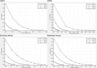
(10) Yl. (1). ∫ f (Y )dy = δP. 0. 0. where f(Y) is the current income distribution. To attain a poverty level δP0 from the current income distribution, individual l’s income will have to reach the poverty line z. Incomes are modified through two channels: fiscal policy and neutral economic growth. For simplicity we explain the first redistributive policy considered: the government taxes incomes at a uniform rate t on top of the current tax system, and distributes the revenues in equal shares per capita e. We also assume neutral economic growth at an annual rate g. Equation (2) shows the combinations of g and fiscal policy (t, e) such that individual l reaches the poverty line in the goal year (2015 in the MDGs) (2) (Yl (1 + g ) n (1 − t ) ) + e = z where n labels the number of years from the current year to the goal year. The government budget constraint requires (3). e = tµ (1 + g ) n. where µ is mean current income. Combining (2) and (3) yields, (4). (Yl (1 − t ) + tµ )(1 + g )n = z. Equation (4) defines the isopoverty curves: combinations of tax rates t and growth rates g that allow reaching the goal δP0 in n years. From (4) it is straightforward to find the tax rate as function of g (5). t=. z − Yl (1 + g ) n (1 + g ) n ( µ − Yl ). or the growth rate as a function of t (6). ⎤ ⎡ z g=⎢ ⎥ ⎣ Yl (1 − t ) + tµ ⎦. 1/ n. −1. For each of the 4 countries of the Southern Cone we compute isopoverty curves using the four alternative definitions of poverty lines. In each case we show several curves, being that which corresponds to the MDG the most relevant one. This curve indicates the possible combinations of growth and redistribution leading to the poverty-reduction MDG.. 9.

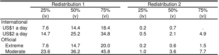
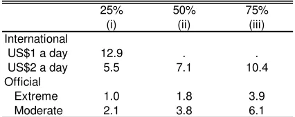
(11) 4. Results for the mechanical microsimulations In this section we present the main results of applying the methodology outlined in section 3 to the microdata of the four Southern Cone countries. Argentina As discussed above, since the early 1990s Argentina has moved away from the poverty MDG. Table 4.1 reproduces poverty in the base year (1992) and presents three targets in terms of poverty reduction: 25%, 50% and 75% from the base year. The column for 50% is the MDG approved by United Nations. Argentina has to substantially reduce poverty from the present to 2015 to meet the MDG. Table 4.2 gives an idea of the size of this effort. To reach the USD2 poverty MDG (50% reduction in poverty measured with the USD2-a-day poverty line) with no changes in inequality, Argentina will have to grow at an annual rate of 9.5% until 2015, which is clearly an extremely unlikely scenario. Even to reach just a 25% reduction in poverty, the annual growth rate should be very high: 8.1%. The simulations generate similar values when using the official moderate and extreme poverty lines.8 In Table 4.3 we show the results of two alternative scenarios to reach the MDG. Under the label “redistribution 1” we present the uniform tax rate (on top of the existing tax system) needed to reach a given poverty-reduction target, assuming no growth, no inefficiencies, and equal expenditures per capita financed with the new tax. The magnitudes of the tax rates involved are again difficult to imagine to be implementable in practice. For instance, to meet the MDG for the moderate official poverty line, the incremental tax rate should be 61.4%. Under the label “redistribution 2” we simulate transfers aimed at attaining a given povertyreduction target at the minimum fiscal cost, financed with a uniform tax levied only on the non-poor. The fiscal cost in this case is substantially lower. However, considering that this is a lower bound very unlikely to be reached, some values are still high. For instance, this well-targeted redistributive policy would need a tax rate of 14.9% to meet the MDG (assuming no growth).. 8. Some people have incomes very close to zero. The income growth rates needed to take them out of poverty are then high. The extreme case is for individuals with zero income. Most people under the USD1 a day in Argentina belong to this group. For this reason we do not present the (extremely high) growth rate needed to reduce poverty. 10.

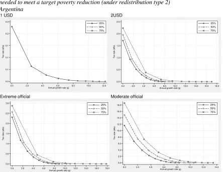
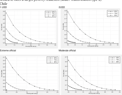
(12) Growth and redistribution can be combined to reduce poverty. The isopoverty curves of Figures 4.1 and 4.2 show these combinations for the four poverty lines under study, and the two alternative redistribution policies. Obviously, the combination of scenarios reduces the requirement of the growth and tax rates needed to reach a given poverty target. However, the values involved are still high. Take the case of the official moderate poverty in Figure 4.1. Even with an initial tax rate of 20%, which is very high, the annual growth rate should be closer to 5%. With a still high incremental tax rate of 10%, the required annual growth rate increases to an unlikely 7.5%. If the policy could be perfectly targeted to reduce the headcount ratio, the growth and redistribution efforts could take values more likely to be achieved. A combined initial incremental tax rate of 5% and an annual growth rate of 3% will be enough to meet the MDG. If this second type of redistribution were possible, and the economy grew at 3%, the tax rate needed to reach the MDG for the international lines would be small (less than 1%). Chile The case of Chile sharply contrasts with that of Argentina: since 1990 poverty has been substantially reduced. In fact, according to the discussion in section 2, Chile has already achieved the goal of halving poverty. For this reason the analysis for Chile differs from that for the other three Southern Cone countries. It would be senseless to simulate the growth and redistribution rates needed to meet the poverty MDG, since Chile has already met that goal. Instead of studying the target of halving poverty, we simulate changes that would allow achieving a more ambitious reduction in poverty: 60%, 70% and 80% from the 1990 values. Table 4.4 suggests that Chile would be able to achieve these targets if the country could sustain the rates of poverty reduction of the 1990s. Poverty measured with the official poverty line dropped 18 points from 1990 to 2000. In the remaining 15 years to 2015 poverty will have to fall another 9 points. As mentioned above, according to MIDEPLAN estimates poverty has already decreased almost 2 points since 2000. Table 4.5 gives an idea of the growth effort to meet these more ambitious targets. In order to reduce poverty 80% from the 1990 values Chile would need a distributionally neutral annual growth rate of around 3%. That rate climbs to 5.5% when poverty is defined with the USD 1 a day poverty line, which reflects the fact that reducing poverty from low levels only with generalized income growth is particularly hard. Table 4.6 shows the redistribution efforts needed to achieve the poverty reduction goals, assuming no income growth. Even in this stagnant scenario Chile could meet the goals with some moderate redistribution effort. The combinations of growth and redistribution of the isopoverty curves look likely to be attained. The figures suggest that with an annual growth. 11.

(13) rate of 2% and some targeting of the redistribution policy, the incremental tax rate needed to reach even the 80%-poverty-reduction goal would be small. Paraguay As explained in section 2, and given data limitations, we assume based on the information available, that Paraguay has not made any progress in poverty reduction since 1990. Table 4.7 shows the headcount ratio for the four different poverty lines in the base year (1990) and three targets for poverty reduction. Halving moderate poverty in Paraguay would require a reduction of 23.2 points in just 13 years.9 Table 4.8 presents measures of the growth effort needed to reduce poverty. In order to achieve the USD2 poverty MDG, at fixed inequality levels, Paraguay will have to grow at an annual rate of 6.8% until 2015, an unlikely scenario given the past economic experience. Reducing poverty to 25% requires an annual growth of 2.7%, which seems more feasible. The results of the simulations are slightly more optimistic in terms of official poverty measures. For instance, to meet the MDG for the moderate official poverty line, the Paraguay’s economy will have to grow at an annual rate of 4.5%. In Table 4.9 we present the results for the two alternative redistributive scenarios. The simulation results of the first panel are hardly feasible in practice. For instance, to meet the MDG for the moderate official poverty line, the tax rate should increase 36.2%. With a completely targeted redistribution scheme (redistribution 2) the incremental tax rates are considerably smaller, although some are still high, considering the likely unfeasibility of this scenario. For instance, for the case of the moderate poverty line, the 50% MDG goal implies increasing the tax rate in 3.6%. Poverty reduction can be achieved by a combination of growth and redistribution policies. In Figures 4.5 and 4.6, the isopoverty curves present these combinations for the four alternative poverty lines, and the two redistribution policies. Considering the moderate official poverty line and the 50% MDG goal, with an incremental tax rate of 10% the annual growth rate should be close to 3%. In a situation where the public transfers could be ideally targeted to reduce the headcount ratio, the growth and redistribution efforts could take more feasible values. The combination of a 2% tax rate and an annual growth rate of 1% will suffice to achieve the MDG. This objective will be even more likely if we consider a USD1-a-day poverty line. Uruguay 9. Official figures for 2002 have been challenged because of sample problems. However, the recently published values for poverty in 2003 confirm the increase in poverty after 2001. 12.

(14) As explained above, and shown in Table 4.10, Uruguay lost more than a decade in the road to the poverty MDG. The efforts needed to reach the goal in time are then substantially greater than a decade ago. Table 4.11 shows that without changes in inequality, the Uruguayan economy would have to grow at almost an annual 4% from now to 2015 to meet the MDG in terms of official moderate poverty, which seems to be an ambitious scenario. The incremental tax rates in Table 4.12 are high in the first simulation and low in the second, especially when considering the international and extreme poverty lines. Figures 4.7 and 4.8 shows some plausible combinations of growth and redistribution that can help Uruguay meet the MDG. For instance if the economy grows at an annual 3%, the required incremental tax rate would be around 5% for the moderate official poverty line and the USD2 a day poverty line. If the policy could be perfectly targeted to reduce the headcount ratio, the incremental tax would be extremely low.. 5. Microeconometric simulations Rather than changing incomes as in the previous section we could change its determinants, that is, the factors that are believed to affect household income. The methodology has two key steps: estimating an income model, and simulating incomes using the estimated parameters. In this paper we estimate log linear models for individual earnings with the usual covariates of a Mincer equation (age, education, regions, area, sectors, formality) using Heckman maximum likelihood techniques.10 The second stage of the methodology requires assuming some changes in the covariates, and simulating household incomes under the assumed distribution of covariates. The simulations are aimed at assessing the impact of changes in some economic variables on poverty and inequality. In particular, we want to evaluate the likely contribution of changes in some selected variables to the attainment of the poverty-reduction Millennium Development Goal. The impulse in each simulation is given by a change in an economic variable (e.g. years of education, unemployment rate). We do not model the process that generate the impulse, but take it as exogenous. Instead, we carefully trace the impact of the impulse on the household income of each individual, and then on measures of poverty and inequality. Simulation 1: Increase in years of education. 10. Gasparini et al. (2003) and Bustelo (2004) estimate quantile regression models but did not find significantly different results from mean models. 13.

(15) This exercise evaluates an increase in x years of education of the population aged 14 to 65. Years of education of each individual are augmented by x, with two exceptions: we do not allow youngsters to have more years of education than what is normal given their age, and we do not allow people to have more years of education than the maximum actually observed in the household survey. Once years of education are increased, we estimate labor income with the coefficients and residuals of the Mincer equation relevant to his or her gender. With the new estimated labor income, we recompute household income, and the measures of poverty and inequality. Simulation 2: Upgrading the educational structure We simulate two situations. In the first one, all the relevant population has at least primary school, which means that we change the educational status of those with no education or primary incomplete. In the second simulation we do not allow anybody to have less than secondary complete, with the exception of those workers younger than 19 years-old. Simulation 3: Reduction in unemployment rate This exercise assesses the impact of a reduction of x% in the unemployment rate. We randomly pick unemployed people and assign them the labor income estimated according to their characteristics and the parameters of the relevant Mincer equation. Simulation 4: Reduction in informality We divide the working population into two categories: informal workers are those salaried workers in small firms, non-professional self-employed, and familiar workers with zero income. We randomly choose some of these workers and pretend they move to the formal sector. We estimate their labor incomes by adding the coefficient of the dummy variable for formality in the labor income equation. Simulation 5: Reduction in agricultural employment This exercise simulates a reduction of x% in agricultural employment. People are moved from the agricultural to the manufacturing industry. The new labor incomes are computed using the dummies for the manufacturing sector in the relevant Mincer equation corresponding to the worker’s gender. Simulation 6: Reduction in the number of children. 14.

(16) We perform two types of simulations. In the first one the number of children (sons and daughters under 12) in a family is reduced by an integer x. In the second one, no family is allowed to have more than y children. Once we change the demographic structure, we recompute per capita or equivalized household income, and estimate poverty and inequality. We ignore the likely changes in labor market participation that may result after the reduction in the number of children in the household.. 6. Results of the microsimulations In this section we present the main results of applying the methodology outlined in section 5 to the microdata of the four Southern Cone countries. Argentina Table 6.1 shows the poverty headcount ratio using different lines and the Gini coefficient over two income distributions under 13 alternative scenarios. Table 6.2 records the changes with respect to the values of the latest survey available (May, 2003). A strong result emerges from the tables: despite the fact that in all scenarios poverty falls, the changes fall short of the required drops to meet the MDG. The gaps are very large. For instance, while poverty has to decrease 43.7 points to reach the MDG poverty value with the official line, a generalized increase in 5 years of education could lead to a fall of approximately 14 points. This is not a small decline in poverty, but it is not enough to reach the goal after the dramatic increase in poverty in Argentina since the early 1990s. All the results in Argentina are affected by the fact that in our last available survey -May 2003- poverty was close to the peak reached during the crisis of 2002. As the economy recovers poverty is expected to substantially fall. In fact, that has happened during 2004 according to the results of the new EPH Continua (see Gasparini 2005, b). Poverty fell more than 10 points since May 2003. These figures reflect the strong effect of crisis and recoveries on poverty that can dwarf the impact of other policies or structural changes. The tables show that an increase of 1 year of education would have a rather modest impact on poverty. Since most workers have primary school, the first simulation of upgrading the educational structure (panel 2) has a small impact on poverty and inequality. In contrast, a shift to a situation where no worker has less than a high-school degree would imply an important drop in poverty (-8.3) and in inequality (-3.4). Again, although the fall in poverty is significant, it appears rather small compared to the drop needed to reach the MDG. The fall in inequality is relatively large. A drop of 3.4 points in the Gini would place inequality close to the levels prior to the Tequila crisis, although still far from the levels of non-crisis years of the 1970s and 1980s.. 15.

(17) A reduction of unemployment in 25% would not have a large impact on poverty (-2.2). Many unemployed people are not poor, so reducing unemployment would not affect poverty. In 2003 30% of the unemployed were not poor according to the official poverty line. Moreover, most poor unemployed people have characteristics (e.g. young, low education) that implies low wages if they find a job. These wages are often not enough to drive them out of poverty. Notice that the effect of a fall in unemployment on poverty would have been even smaller if we had assumed that, according to the law, benefits of the Programa Jefes de Hogar are eliminated once a person finds a job. A more ambitious reduction in unemployment (75%) obviously has a larger impact on poverty. The headcount ratio with the moderate poverty line would be reduced in more than 5 points. In panel 4 we simulate changes in the informality rate. The Mincer equations indicates that having a formal job increases earnings in 46% for men and 53% for women. In the more ambitious simulation (a reduction of the informality rate in 75%) poverty falls 4.3 points, which is not a very impressive figure. Again, many informal workers are not poor (42%), while many of those who are poor are anyway far from the poverty line to reach it with the wage increase associated to formality. Finally, the reduction in the number of children appears to have a significant impact on extreme poverty. For instance, a situation with 1 child less per household would imply a fall of more than 2 points in USD1 poverty, which implies a drop comparable to a reduction in unemployment in 75%, or an increase of 3 years of education. In contrast, the impact of the simulated change in fertility on moderate poverty is not large. Chile As commented above Chile has already met the poverty MDG. In tables 6.3 and 6.4 we consider the target of reducing poverty 70% from the 1990 values. According to the results of the simulations reported in the tables a moderate increase in the educational level of the Chilean population can have a sizeable impact on poverty. A more ambitious scenario, e.g. an increase in 5 years of education, could be enough alone to reach the augmented MDG (70%). A program that help reaching full coverage of primary school would not have a very large impact on poverty, since attendance rates are already high. In contrast, full coverage in secondary school implies substantially larger impacts. The second panel in table 6.4 shows that an upgrading of the educational structure such that no worker has less than secondary school implies, keeping all other things constant (e.g. returns to education), a sizeable reduction of nearly 7 points in official moderate poverty.. 16.

(18) Reduction in labor informality is often seen as an instrument for increasing incomes and reducing poverty. In Chile, however, when controlling for other characteristics, the formal dummy in the earnings equation is positive but small (in fact, not statistically significant). That means that moving people from the informal to the formal sector without changing their characteristics (e.g. education) will have a minor impact on poverty (see tables 6.3 and 6.4). The same argument applies to the agricultural employment. Wages in that sector are lower than in the manufacturing industry. However, when controlling for other worker characteristics (basically, education) the differences vanish. Moving people from the rural areas to manufacturing industries in urban areas does not seem helpful for the reduction of poverty in Chile. Finally, reducing the number of children per household has at least a short-run poverty-decreasing effect. Paraguay Paraguay has a long way to go in order to meet the poverty MDG. None of the scenarios simulated in tables 6.5 and 6.6 would be enough to reach the poverty target. However, the results suggest that some changes could have sizeable impacts on poverty rates. The educational upgrading of the population would be particularly effective. Keeping all other things constant, official moderate poverty could be reduced by 10 points with a strong educational policy that increases years of education by 5 (or that achieves full coverage of high-school). The reduction in unemployment, informality, and agricultural employment all have poverty-decreasing effects. The reduction in informality seems to be particularly effective. The demographic simulations also imply relative large reductions in poverty. In the two simulation of panel 6 moderate poverty falls around 4 points. Uruguay In the last decade Uruguay has moved away from the road to meeting the poverty MDG. Tables 6.7 and 6.8 show the likely direct impact on poverty reduction of changes in some socioeconomic scenarios that can help the country to advance towards the MDG. Uruguay is one of the countries with the highest levels of education in Latin America. However, there is still a large fraction of the population with low educational levels and high returns to education. A generalized increase in 5 years of education could imply a fall in poverty of 14 points, which could help Uruguay reaching the poverty MDG. Since most Uruguayans have a primary school degree, the challenge is to make high school universal. The second panel in table 6.8 shows that such policy would have a sizeable impact on poverty and inequality.. 17.

(19) Unemployment was very high in 2003 (16.3% for adults). A generalized reduction in unemployment could generate large drops in poverty and inequality. However, the third panel in table 6.8 suggests that lowering unemployment would not be enough to reach the poverty MDG. Formal workers earn on average 60% more than informal workers, controlling for other characteristics. Reducing informality can have a relevant povertyreducing impact. A 25% reduction in informality, for instance could be associated to a fall in poverty of around 9 points (using the official poverty line). Finally, a reduction in the size of households could contribute to a reduction in income poverty (at least in the short-run). The contribution, however, seems small.. 7. An assessment In this paper we use microsimulations techniques based on microdata from household surveys to provide rough estimates of alternatives scenarios needed to reach the poverty MDG in the Southern Cone countries. Table 7.1 summarizes the main results of the mechanical simulations of changing incomes. Argentina has moved away from the MDG since the early 1990s, which implies that today the probability for that country to meet the MDG is small. Argentina would require sustained high economic growth combined with a strong and targeted redistributive policy, a scenario that the country has not experienced in a very long time (if ever). Paraguay and Uruguay face similar situations, although the growth and redistribution efforts needed to reach the MDG are smaller. In contrast, Chile has already attain the poverty reduction MDG, and it is likely to further reduce poverty with small growth and redistribution efforts. The paper highlights the importance of acting in several directions in order to reduce poverty. High economic growth is certainly desirable, although in some countries it seems that it is not enough to reach the poverty MDG. On the other hand, redistributive policies help reducing poverty. However, the paper stresses that without growth the tax rate needed to meet the MDG in most countries is very high, which is politically difficult to implement, and also very likely detrimental to growth. The paper shows that efforts in targeting the transfers to the poor alleviate the need for high inefficient tax rates, and hence can make the whole package politically implementable and internally consistent. Table 7.2 summarizes the results of the microeconometric simulations. Increasing years of education has a sizeable effect on poverty, in particular achieving full attendance rates in high school. The reduction in unemployment and informality, and in household size would. 18.

(20) be particularly poverty-reducing in Argentina and Paraguay. However, none of these scenarios alone are enough to reach the poverty MDG in these countries. The methodology used in this paper should be viewed as just a preliminary evaluation of the direct impact of certain impulses on poverty and inequality. Increasing years of education or reducing the fertility rate have many other consequences than the ones analyzed in this paper. Knowing and computing all the interactions, theoretically and empirically, is far beyond the capacity of the social sciences in their current state. The simulations should then be taken just as one of many inputs in the evaluation of economic scenarios and policies. We believe they are relevant inputs that have an important advantage: they can be replicated and improved in concrete ways to provide more helpful results.. 19.

(21) References Chen, S. and Ravallion., M. (2001). How did the world's poorest fare in the 1990s? World Bank working paper. Fazio, V. (2005 a). Monitoring the socio-economic conditions in Paraguay. Working paper CEDLAS-The World Bank. Fazio, V. (2005 b). Poverty and Inequality in Paraguay: Methodological Issues and a Literature Review. Working paper CEDLAS-The World Bank. Gasparini, L. (2005 a).Monitoring the socio-economic conditions in Argentina. Working paper CEDLAS-The World Bank. Gasparini, L. (2005 b). Poverty and Inequality in Argentina: Methodological Issues and a Literature Review. Working paper CEDLAS-The World Bank. Gasparini, L., Cicowiez, M., Gutiérrez, F. and Marchionni, M. (2003). Simulating Income Distribution Changes in Bolivia: a Microeconometric Approach. Bolivia Poverty Assessment, The World Bank. Paes de Barros et al. (2003). Meeting the Millennium Poverty Reduction targets in Latin America. UNDP. Pizzolito , G. (2005 a). Monitoring the socio-economic conditions in Chile. Working paper CEDLAS-The World Bank. Pizzolito (2005 b). Poverty and Inequality in Chile: Methodological Issues and a Literature Review. Working paper CEDLAS-The World Bank. Ravallion, M., Datt, G. and van de Walle, D. (1991). Quatifying absolute poverty in the Developing World. Review of Income and Wealth 37, 345-361. Winkler, H. (2005 a). Uruguay. Monitoring the socio-economic conditions in Uruguay. Working paper CEDLAS-The World Bank. Winkler, H. (2005 b). Poverty and Inequality in Uruguay: Methodological Issues and a Literature Review. Working paper CEDLAS-The World Bank. Wold Bank (2004). World Development Indicators 2004.. 20.

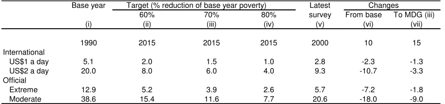
(22) Table 2.1 Poverty headcount ratio Argentina, Chile, Paraguay and Uruguay. 1. Argentina. Base year (i). Target (ii). Latest survey (iii). Changes From base To target (iv) (v). 1992. 2015. 2003. 11. 12. International USD1 a day USD2 a day Official Extreme Moderate. 1.5 4.9. 0.8 2.5. 8.0 23.5. 6.5 18.6. -7.2 -21.0. 4.5 22.6. 2.3 11.3. 25.9 55.0. 21.4 32.4. -23.7 -43.7. 2. Chile. 1990. 2015. 2000. 10. 15. 5.1 20.0. 2.6 10.0. 2.8 9.3. -2.3 -10.7. -0.2 0.7. 12.9 38.6. 6.5 19.3. 5.7 20.6. -7.2 -18.0. 0.8 -1.3. 1990. 2015. 2002. 12. 13. International USD1 a day USD2 a day Official Extreme Moderate. 3. Paraguay International USD1 a day USD2 a day Official Extreme Moderate. 21.2 37.2. 10.6 18.6. 21.2 37.2. 0.0 0.0. -10.6 -18.6. 21.7 46.4. 10.9 23.2. 21.7 46.4. 0.0 0.0. -10.9 -23.2. 4. Uruguay. 1989. 2015. 2003. 14. 12. 0.3 1.9. 0.1 0.9. 1.2 5.7. 0.9 3.8. -1.0 -4.8. 2.8 27.6. 1.4 13.8. 2.8 31.3. 0.1 3.7. -1.4 -17.5. International USD1 a day USD2 a day Official Extreme Moderate. Source: own calculations based on microdata from household surveys.. Table 2.2 Annual required change in poverty (percentual points) from 2004 to 2015 to reach the poverty MDG Argentina, Chile, Paraguay and Uruguay. Argentina Chile Paraguay Uruguay. International PL USD1 USD2 -0.6 -1.6 Already met Already met -0.8 -1.4 -0.1 -0.4. Official PL Extreme Moderate -1.8 -3.4 Already met Already met -0.8 -1.8 -0.1 -1.5. Source: own calculations based on microdata from household surveys.. 21.

(23) Table 4.1 Actual and target poverty headcount ratio Argentina Base year (i). International US$1 a day US$2 a day Official Extreme Moderate. Target (% reduction of base year poverty) 25% 50% 75% (ii) (iii) (iv). Latest survey (v). Changes From base To MDG (iii) (vi) (vii). 1992. 2015. 2015. 2015. 2003. 11. 12. 1.5 4.9. 1.1 3.7. 0.8 2.5. 0.4 1.2. 8.0 23.5. 6.5 18.6. -7.2 -21.0. 4.5 22.6. 3.4 17.0. 2.3 11.3. 1.1 5.7. 25.9 55.0. 21.4 32.4. -23.7 -43.7. Source: own calculations based on microdata from the EPH.. Table 4.2 Annual distributionally-neutral growth rate from 2004 to 2015 needed to meet a target poverty reduction Argentina. International US$1 a day US$2 a day Official Extreme Moderate. 25% (i). 50% (ii). 75% (iii). 12.2 8.1. . 9.5. . 17.0. 8.9 8.3. 11.0 10.5. 17.8 13.5. Source: own calculations based on microdata from the EPH.. Table 4.3 Tax rate needed to meet a target poverty reduction Argentina 25% (iv). Redistribution 1 50% (v). 75% (vi). Redistribution 2 25% 50% (iv) (v). 75% (vi). International US$1 a day 11.4 14.3 14.3 0.2 . . US$2 a day 20.2 21.6 25.8 1.7 2.0 2.2 Official Extreme 23.5 25.4 28.8 2.3 2.6 2.9 Moderate 58.5 61.4 63.8 11.6 14.9 18.6 Source: own calculations based on microdata from the EPH. Note: Redistribution 1=tax rate t on all the population, and equal expenditures per capita. Redistribution 2=tax rate t on all the non-poor, and minimum expenditures needed to reduce poverty headcount ratio.. 22.

(24) Figure 4.1 Isopoverty curves Tax rate and annual distributionally-neutral growth rate needed to meet a target poverty reduction (under redistribution type 1) Argentina 1 USD. 2USD. 14.0. 25% 50% 75%. 12.0. 25% 50% 75%. 25.0. 20.0. Tax rate (alfa). Tax rate (alfa). 10.0. 8.0. 6.0. 15.0. 10.0. 4.0 5.0. 2.0. 0.0. 0.0 0.0. 5.0. 10.0 15.0 Annual growth rate (g). 20.0. 0.0. 25.0. Extreme official. 2.0. 4.0. 6.0. 8.0 10.0 Annual growth rate (g). 12.0. 14.0. 16.0. 18.0. Moderate official. 30.0. 70.0. 25% 50% 75%. 25.0. 25% 50% 75%. 60.0. 50.0 Tax rate (alfa). Tax rate (alfa). 20.0. 15.0. 40.0. 30.0. 10.0 20.0. 5.0. 10.0. 0.0. 0.0. 0.0. 2.0. 4.0. 6.0. 10.0 8.0 Annual growth rate (g). 12.0. 14.0. 16.0. 18.0. 0.0. 2.0. 4.0. 6.0 8.0 Annual growth rate (g). 10.0. 12.0. 14.0. Source: own calculations based on microdata from the EPH.. 23.

(25) Figure 4.2 Isopoverty curves Tax rate and annual distributionally-neutral growth rate needed to meet a target poverty reduction (under redistribution type 2) Argentina 1 USD. 2USD 2.5. 25% 50% 75%. 0.2. 2.0. 0.1. 1.5. Tax rate (alfa). Tax rate (alfa). 0.3. 0.1. 0.1. 25% 50% 75%. 1.0. 0.5. 0.0. 0.0 4.0. 2.0. 0.0. 6.0 Annual growth rate (g). 8.0. 12.0. 10.0. Extreme official. 0.0. 6.0. 4.0. 2.0. 10.0 8.0 Annual growth rate (g). 14.0. 12.0. 16.0. 18.0. Moderate official. 3.0. 25% 50% 75%. 2.5. 25% 50% 75%. 18.0. 16.0 14.0. 12.0. Tax rate (alfa). Tax rate (alfa). 2.0. 1.5. 10.0. 8.0. 6.0. 1.0. 4.0. 0.5 2.0. 0.0. 0.0. 0.0. 2.0. 4.0. 6.0. 8.0 10.0 Annual growth rate (g). 12.0. 14.0. 16.0. 18.0. 0.0. 2.0. 4.0. 6.0 8.0 Annual growth rate (g). 10.0. 12.0. 14.0. Source: own calculations based on microdata from the EPH.. 24.

(26) Table 4.4 Actual and target poverty headcount ratio Chile Base year. Target (% reduction of base year poverty) 60% 70% 80% (ii) (iii) (iv). (i). International US$1 a day US$2 a day Official Extreme Moderate. Latest survey (v). Changes From base To MDG (iii) (vi) (vii). 1990. 2015. 2015. 2015. 2000. 10. 15. 5.1 20.0. 2.0 8.0. 1.5 6.0. 1.0 4.0. 2.8 9.3. -2.3 -10.7. -1.3 -3.3. 12.9 38.6. 5.2 15.4. 3.9 11.6. 2.6 7.7. 5.7 20.6. -7.2 -18.0. -1.8 -9.0. Source: own calculations based on microdata from the CASEN.. Table 4.5 Annual distributionally-neutral growth rate from 2004 to 2015 needed to achieve target poverty reduction Chile. International US$1 a day US$2 a day Official Extreme Moderate. 60% (i). 70% (ii). 80% (iii). 1.4 0.5. 3.0 1.5. 5.5 3.2. 0.0 0.9. 0.9 1.8. 2.3 3.2. Source: own calculations based on microdata from the CASEN.. Table 4.6 Tax rate needed to meet a target poverty reduction Chile 60% (iv) International US$1 a day US$2 a day Official Extreme Moderate. Redistribution 1 70% 80% (v) (vi). 60% (iv). Redistribution 2 70% (v). 80% (vi). 1.69 1.52. 3.25 4.00. 4.88 7.19. 0.01 0.01. 0.02 0.06. 0.04 0.15. 0.03 4.62. 2.04 8.51. 4.60 12.76. 0.00 0.08. 0.01 0.29. 0.05 0.63. Source: own calculations based on microdata from the CASEN. Note: Redistribution 1=tax rate t on all the population, and equal expenditures per capita. Redistribution 2=tax rate t on all the non-poor, and minimum expenditures needed to reduce poverty headcount ratio.. 25.

(27) Figure 4.3 Isopoverty curves Tax rate and annual distributionally-neutral growth rate needed to meet a target poverty reduction (under redistribution type 1) Chile 1 USD. 2USD. 5.0. 60% 70% 80%. 4.5. 7.0. 6.0. 4.0 3.5. 5.0. 3.0. Tax rate (alfa). Tax rate (alfa). 60% 70% 80%. 2.5 2.0. 4.0. 3.0. 1.5. 2.0 1.0. 1.0. 0.5 0.0. 0.0 -0.0. 1.0. 2.0. 3.0 Annual growth rate (g). 4.0. 5.0. 6.0. Extreme official. 2.0 1.5 Annual growth rate (g). 1.0. 0.5. -0.0. 2.5. 3.0. 3.5. Moderate official 14.0. 60% 70% 80%. 4.5 4.0. 60% 70% 80%. 12.0. 3.5 10.0 Tax rate (alfa). Tax rate (alfa). 3.0 2.5 2.0 1.5. 8.0. 6.0. 4.0. 1.0 2.0. 0.5 0.0. 0.0. -0.0. 0.5. 1.5 1.0 Annual growth rate (g). 2.0. 2.5. -0.0. 0.5. 1.0. 1.5 2.0 Annual growth rate (g). 2.5. 3.0. 3.5. Source: own calculations based on microdata from the CASEN 2000. 26.

(28) Figure 4.4 Isopoverty curves Tax rate and annual distributionally-neutral growth rate needed to meet a target poverty reduction (under redistribution type 2) Chile 1 USD. 2USD 0.2. 0.0. 60% 70% 80%. 0.0. 0.1. 0.0. ¨¨¨¨. 0.0. Tax rate (alfa). Tax rate (alfa). 60% 70% 80%. 0.1. 0.0. 0.1. 0.1. 0.0. 0.1. 0.0. 0.0. 0.0. 0.0. 0.0. 0.0. 0.0. 2.0. 1.0. 3.0 Annual growth rate (g). 4.0. 5.0. 0.0. 6.0. Extreme official. 0.5. 1.0. 1.5 2.0 Annual growth rate (g). 2.5. 3.5. 3.0. Moderate official. 0.1. 0.7. 60% 70% 80%. 0.0. 60% 70% 80%. 0.6. 0.0. 0.5. Tax rate (alfa). Tax rate (alfa). 0.0 0.0 0.0 0.0 0.0. 0.4. 0.3. 0.2. 0.0. 0.1 0.0. 0.0. 0.0. 0.0. 0.5. 1.5 1.0 Annual growth rate (g). 2.0. 2.5. 0.0. 0.5. 1.0. 1.5 2.0 Annual growth rate (g). 2.5. 3.0. 3.5. Source: own calculations based on microdata from the CASEN 2000. 27.

(29) Table 4.7 Actual and target poverty headcount ratio Paraguay Base year (i). International US$1 a day US$2 a day Official Extreme Moderate. Target (% reduction of base year poverty) 25% 50% 75% (ii) (iii) (iv). Latest survey (v). Changes From base To MDG (iii) (vi) (vii). 1992. 2015. 2015. 2015. 2003. 11. 12. 21.2 37.2. 15.9 27.9. 10.6 18.6. 5.3 9.3. 21.2 37.3. 0.0 0.0. -10.6 -18.7. 21.7 46.4. 16.3 34.8. 10.9 23.2. 5.4 11.6. 21.7 46.4. 0.0 0.0. -10.9 -23.2. Source: own calculations based on microdata from the EPH.. Table 4.8 Annual distributionally-neutral growth rate from 2003 to 2015 needed to meet a target poverty reduction Paraguay. International US$1 a day US$2 a day Official Extreme Moderate. 25% (i). 50% (ii). 75% (iii). 3.5 2.7. 11.0 6.8. . 20.6. 1.6 2.1. 3.9 4.5. 6.7 8.3. Source: own calculations based on microdata from the EPH.. Table 4.9 Tax rate needed to meet a target poverty reduction Paraguay 25% (iv) International US$1 a day US$2 a day Official Extreme Moderate. Redistribution 1 50% (v). 75% (vi). 25% (iv). Redistribution 2 50% (v). 75% (vi). 7.6 14.7. 14.4 25.2. 18.4 34.8. 0.2 0.5. 0.7 2.1. . 4.9. 7.6 23.6. 14.7 36.2. 20.0 45.8. 0.2 1.0. 0.6 3.6. 1.5 7.7. Source: own calculations based on microdata from the EPH (2002). Note: Redistribution 1=tax rate t on all the population, and equal expenditures per capita. Redistribution 2=tax rate t on all the non-poor, and minimum expenditures needed to reduce poverty headcount ratio.. 28.

(30) Figure 4.5 Isopoverty curves Tax rate and annual distributionally-neutral growth rate needed to meet a target poverty reduction (under redistribution type 1) Paraguay USD1. USD2 35.0. 25% 50% 75%. 18.0 16.0. 2 5% 5 0% 7 5%. 30.0. 14.0 25.0 Tax rate ( alfa). Tax rate ( alfa). 12.0 10.0 8.0. 20.0. 15.0. 6.0 10.0 4.0 5.0 2.0 0.0. 0.0 -0.0. 5.0. 10.0 15.0 Annual g rowth rate (g ). 20.0. 25.0. Extreme official. 0.0. 2.0. 4.0. 6.0. 8.0 10.0 12.0 Annual g rowth rate (g ). 14.0. 16.0. 18.0. Moderate official Extreme. 20.0. 45.0. 25% 50% 75%. 18.0. 25 % 50 % 75 %. 40.0. 16.0. 20.0. 35.0. 14.0 Tax rate ( alfa). Tax rate (alfa). 30.0 12.0 10.0 8.0. 25.0 20.0 15.0. 6.0. 10.0. 4.0. 5.0. 2.0. 0.0. 0.0 -0.0. 1.0. 2.0. 3.0 4.0 Annual g rowth rate (g ). 5.0. 6.0. 7.0. -0.0. 1.0. 2.0. 3.0. 4.0 5.0 Annual g rowth rate (g ). 6.0. 7.0. 8.0. 9.0. Source: own calculations based on microdata from the EPH (2002).. 29.

(31) Figure 4.6 Isopoverty curves Tax rate and annual distributionally-neutral growth rate needed to meet a target poverty reduction (under redistribution type 2) Paraguay USD1. USD2 5.0. 25 % 50 % 75 %. 0.7. 0.6. 2 5% 5 0% 7 5%. 4.5 4.0 3.5 Tax rate ( alfa). Tax rate (alfa). 0.5. 0.4. 0.3. 3.0 2.5 2.0 1.5. 0.2. 1.0 0.1 0.5 0.0. 0.0 0.0. 2.0. 4.0. 6.0 Annual g rowth rate (g ). 8.0. 10.0. 12.0. Extreme official. 2.0. 4.0. 6.0. 8.0 10.0 12.0 Annual g rowth rate (g ). 14.0. 16.0. 18.0. 20.0. Moderate official. 1.6. 8.0. 25 % 50 % 75 %. 1.4. 1.2. 6.0. 1.0. 5.0. 0.8. 0.6. 25% 50% 75%. 7.0. Tax rate (alfa). Tax rate ( alfa). 0.0. 4.0. 3.0. 0.4. 2.0. 0.2. 1.0. 0.0. 0.0 0.0. 1.0. 2.0. 3.0 4.0 Annual g rowth rate (g ). 5.0. 6.0. 7.0. 0.0. 1.0. 2.0. 3.0. 4.0 5.0 Annual g rowth rate (g ). 6.0. 7.0. 8.0. 9.0. Source: own calculations based on microdata from the EPH (2002).. 30.

(32) Table 4.10 Actual and target poverty headcount ratio Uruguay Base year (i). International US$1 a day US$2 a day Official Extreme Moderate. Target (% reduction of base year poverty) 25% 50% 75% (ii) (iii) (iv). Latest survey (v). Changes From base To MDG (iii) (vi) (vii). 1989. 2015. 2015. 2015. 2003. 14. 12. 0.3 1.9. 0.2 1.4. 0.1 0.9. 0.1 0.5. 1.2 5.7. 0.9 3.8. -1.0 -4.8. 2.8 27.6. 2.1 20.7. 1.4 13.8. 0.7 6.9. 2.8 31.3. 0.1 3.7. -1.4 -17.5. Source: own calculations based on microdata from the ECH.. Table 4.11 Annual distributionally-neutral growth rate from 2003 to 2015 needed to meet a target poverty reduction Uruguay. International US$1 a day US$2 a day Official Extreme Moderate. 25% (i). 50% (ii). 75% (iii). 12.9 5.5. . 7.1. . 10.4. 1.0 2.1. 1.8 3.8. 3.9 6.1. Source: own calculations based on microdata from the ECH.. Table 4.12 Tax rate needed to meet a target poverty reduction Uruguay 25% (iv) International US$1 a day US$2 a day Official Extreme Moderate. Redistribution 1 50% (v). 75% (vi). 25% (iv). Redistribution 2 50% (v). 75% (vi). 8.0 10.7. 10.1 12.4. 10.1 15.0. 0.0 0.2. . 0.2. . 0.3. 2.4 18.2. 4.1 27.0. 7.5 34.0. 0.0 0.7. 0.0 1.8. 0.1 3.5. Source: own calculations based on microdata from the ECH 2003. Note: Redistribution 1=tax rate t on all the population, and equal expenditures per capita. Redistribution 2=tax rate t on all the non-poor, and minimum expenditures needed to reduce poverty headcount ratio.. 31.

(33) Figure 4.7 Isopoverty curves Tax rate and annual distributionally-neutral growth rate needed to meet a target poverty reduction (under redistribution type 1) Uruguay 1 USD. 2USD. 10.0. 16.0. 25% 50% 75%. 9.0. 25% 50% 75%. 14.0. 8.0 12.0. Tax rate (alfa). Tax rate (alfa). 7.0 6.0 5.0 4.0. 10.0. 8.0. 6.0. 3.0 4.0 2.0 2.0. 1.0. 0.0. 0.0 -0.0. 5.0. 10.0. 15.0 20.0 A nnual growth rate (g). 25.0. -0.0. 30.0. Extreme official. 2.0. 3.0. 4.0 5.0 6.0 A nnual growth rate (g). 7.0. 8.0. 9.0. 10.0. Moderate official. 8.0. 35.0. 25% 50% 75%. 7.0. 25% 50% 75%. 30.0. 6.0. 25.0. 5.0. Tax rate (alfa). Tax rate (alfa). 1.0. 4.0. 3.0. 20.0. 15.0. 10.0 2.0 5.0. 1.0. 0.0. 0.0 -0.0. 0.5. 1.0. 1.5 2.0 2.5 A nnual growth rate (g). 3.0. 3.5. 4.0. -0.0. 1.0. 2.0. 3.0 4.0 A nnual growth rate (g). 5.0. 6.0. Source: own calculations based on microdata from the ECH 2003.. 32.

(34) Figure 4.8 Isopoverty curves Tax rate and annual distributionally-neutral growth rate needed to meet a target poverty reduction (under redistribution type 2) Uruguay 1 USD. 2USD. 0.0. 0.3. 25% 50% 75%. 0.0. 0.3. 0.2 Tax rate (alfa). 0.0 Tax rate (alfa). 25% 50% 75%. 0.0. 0.1. 0.0. 0.1. 0.0. 0.1. 0.0. 0.0 0.0. 2.0. 4.0. 6.0 8.0 A nnual growth rate (g). 10.0. 12.0. 14.0. Extreme official. 0.0. 1.0. 2.0. 3.0. 4.0 5.0 6.0 A nnual growth rate (g). 7.0. 8.0. 9.0. 10.0. Moderate official 35.0. 25% 50% 75%. 0.1. 25% 50% 75%. 30.0. 0.1 25.0 Tax rate (alfa). Tax rate (a lfa). 0.0. 0.0. 20.0. 15.0. 0.0 10.0. 0.0. 5.0. 0.0. 0.0 0.0. 0.5. 1.0. 1 .5 2.0 2.5 A n nual growth rate (g). 3.0. 3.5. 4 .0. -0.0. 1.0. 2.0. 3.0 4.0 A nnual growth rate (g). 5.0. 6.0. Source: own calculations based on microdata from the ECH 2003.. 33.

(35) Table 6.1 Microsimulations Poverty headcount and the Gini coefficient Argentina Poverty headcount ratio International Official USD 1 USD 2 Extreme Moderate. Gini coefficient Per capita Equivalized income income. Actual values (2003) MDG values (2015). 8.0 0.8. 23.5 2.5. 25.9 2.3. 55.0 11.3. 0.520. 0.498. 1. Increase in years of education Increase in 1 year Increase in 3 year Increase in 5 year. 7.2 6.2 5.5. 21.4 18.3 15.6. 24.2 20.0 16.9. 52.4 46.4 41.1. 0.517 0.510 0.502. 0.495 0.489 0.482. 2. Upgrading in educational structure Nobody without primary school Nobody without secondary school. 7.5 5.6. 21.9 16.3. 24.2 18.4. 54.0 46.7. 0.515 0.487. 0.492 0.464. 3. Reduction in unemployment rate 25 % reduction 50 % reduction 75 % reduction. 6.9 6.4 5.8. 21.9 20.6 19.3. 24.1 22.9 21.7. 52.8 51.2 49.5. 0.514 0.510 0.505. 0.492 0.488 0.483. 4. Reduction in informality rates 25% reduction 50% reduction 75% reduction. 7.4 7.0 6.7. 22.2 21.0 19.9. 24.4 23.0 22.0. 53.6 52.2 50.7. 0.517 0.514 0.510. 0.494 0.492 0.487. 5. Reduction in the number of children 1 child less in each household No household with more than 2 children. 5.9 6.1. 20.5 20.1. 23.0 22.8. 52.5 53.3. 0.512 0.509. 0.493 0.489. 34.

(36) Table 6.2 Microsimulations Changes in poverty headcount and the Gini coefficient Argentina Poverty headcount ratio International Official USD 1 USD 2 Extreme Moderate. Gini coefficient Per capita Equivalized income income. Required change in poverty to meet the MDG. -7.2. -21.0. -23.7. -43.7. 1. Increase in years of education Increase in 1 year Increase in 3 year Increase in 5 year. -0.8 -1.8 -2.5. -2.1 -5.2 -7.9. -1.8 -5.9 -9.1. -2.6 -8.6 -13.9. -0.3 -1.0 -1.9. -0.3 -0.9 -1.6. 2. Upgrading in educational structure Nobody without primary school Nobody without secondary school. -0.5 -2.3. -1.5 -7.2. -1.7 -7.6. -1.0 -8.2. -0.5 -3.3. -0.6 -3.4. 3. Reduction in unemployment rate 25 % reduction 50 % reduction 75 % reduction. -1.1 -1.5 -2.2. -1.6 -2.9 -4.2. -1.8 -3.0 -4.2. -2.2 -3.7 -5.4. -0.6 -1.1 -1.6. -0.6 -1.0 -1.5. 4. Reduction in informality rates 10% reduction 25% reduction 75% reduction. -0.5 -0.9 -1.3. -1.2 -2.5 -3.6. -1.5 -2.9 -3.9. -1.4 -2.8 -4.3. -0.4 -0.6 -1.1. -0.4 -0.6 -1.1. 5. Reduction in the number of children 1 child less in each household No household with more than 2 children. -2.1 -1.9. -2.9 -3.4. -3.0 -3.1. -2.4 -1.7. -0.9 -1.1. -0.5 -0.9. 35.

(37) Table 6.3 Microsimulations Poverty headcount and the Gini coefficient Chile Poverty headcount ratio International Official USD 1 USD 2 Extreme Moderate. Gini coefficient Per capita Equivalized income income. Actual values (2000) MDG values (2015). 2.8 1.5. 9.3 6.0. 5.7 3.9. 20.6 11.6. 0.572. 0.561. 1. Increase in years of education Increase in 1 year Increase in 3 year Increase in 5 year. 2.6 2.3 2.0. 8.3 6.6 5.3. 5.1 4.2 3.4. 18.2 13.5 10.3. 0.584 0.611 0.616. 0.575 0.604 0.611. 2. Upgrading in educational structure Nobody without primary school Nobody without secondary school. 2.6 2.0. 8.4 6.0. 5.3 3.8. 19.1 13.7. 0.565 0.538. 0.555 0.526. 3. Reduction in informality rates 25% reduction 50% reduction 75% reduction. 2.8 2.7 2.7. 9.3 9.2 9.1. 5.7 5.6 5.6. 20.5 20.3 20.2. 0.572 0.571 0.571. 0.561 0.561 0.560. 4. Reduction in agricultural employment 10% reduction 25% reduction 50% reduction. 2.8 2.8 2.8. 9.3 9.3 9.3. 5.7 5.7 5.7. 20.6 20.6 20.6. 0.572 0.572 0.572. 0.561 0.561 0.561. 5. Reduction in the number of children 1 child less in each household No household with more than 2 children. 2.4 2.6. 8.1 8.6. 4.7 5.1. 17.5 19.3. 0.569 0.570. 0.560 0.560. 36.

(38) Table 6.4 Microsimulations Changes in poverty headcount and the Gini coefficient Chile Poverty headcount ratio International Official USD 1 USD 2 Extreme Moderate. Gini coefficient Per capita Equivalized income income. Required change in poverty to meet the MDG. -1.3. -3.3. -1.8. -9.0. 1. Increase in years of education Increase in 1 year Increase in 3 year Increase in 5 year. -0.2 -0.5 -0.8. -1.0 -2.8 -4.1. -0.5 -1.5 -2.2. -2.4 -7.1 -10.3. 1.2 3.9 4.4. 1.3 4.3 4.9. 2. Upgrading in educational structure Nobody without primary school Nobody without secondary school. -0.2 -0.8. -1.0 -3.4. -0.4 -1.8. -1.5 -6.9. -0.7 -3.4. -0.7 -3.6. 3. Reduction in informality rates 10% reduction 25% reduction 75% reduction. 0.0 0.0 -0.1. -0.1 -0.1 -0.2. 0.0 0.0 -0.1. -0.1 -0.3 -0.4. 0.0 -0.1 -0.1. 0.0 -0.1 -0.1. 4. Reduction in agricultural employment 10% reduction 25% reduction 50% reduction. 0.0 0.0 0.0. 0.0 0.0 -0.1. 0.0 0.0 0.0. 0.0 0.0 -0.1. 0.0 0.0 0.0. 0.0 0.0 0.0. 5. Reduction in the number of children 1 child less in each household No household with more than 2 children. -0.4 -0.2. -1.3 -0.7. -1.0 -0.6. -3.1 -1.4. -0.3 -0.1. -0.2 -0.1. 37.

(39) Table 6.5 Microsimulations Poverty headcount Paraguay Poverty headcount ratio International Official USD 1 USD 2 Extreme Moderate. Gini coefficient Per capita Equivalized income income. Actual values (2003) MDG values (2015). 21.2 10.6. 37.2 18.6. 21.7 10.9. 46.4 23.2. 0.571. 0.552. 1. Increase in years of education Increase in 1 year Increase in 3 year Increase in 5 year. 20.9 19.6 18.8. 35.9 33.5 31.5. 20.5 17.5 15.5. 44.8 40.1 35.9. 0.572 0.574 0.576. 0.553 0.556 0.559. 2. Upgrading in educational structure Nobody without primary school Nobody without secondary school. 20.6 18.1. 36.0 29.5. 20.5 15.4. 44.9 35.6. 0.568 0.566. 0.549 0.549. 3. Reduction in unemployment rate 25 % reduction 50 % reduction 75 % reduction. 20.2 19.6 18.6. 35.8 34.2 32.1. 21.1 20.3 19.3. 45.2 43.2 41.7. 4. Reduction in informality rates 25% reduction 50% reduction 75% reduction. 20.5 19.2 18.7. 35.8 33.3 30.9. 20.7 18.8 17.2. 44.2 41.3 38.5. 0.567 0.561 0.555. 0.548 0.542 0.536. 5. Reduction in agricultural employment 10% reduction 25% reduction 50% reduction. 21.1 20.7 20.0. 37.0 36.6 35.4. 22.0 21.7 20.6. 46.5 45.7 44.6. 0.574 0.572 0.572. 0.556 0.554 0.554. 6. Reduction in the number of children 1 child less in each household No household with more than 2 children. 19.5 18.5. 34.2 33.2. 18.9 18.5. 42.8 42.4. 0.564 0.557. 0.548 0.544. 38.

(40) Table 6.6 Microsimulations Changes in poverty headcount Paraguay Poverty headcount ratio International Official USD 1 USD 2 Extreme Moderate. Gini coefficient Per capita Equivalized income income. Required change in poverty to meet the MDG. -10.6. -18.6. -10.9. -23.2. 1. Increase in years of education Increase in 1 year Increase in 3 year Increase in 5 year. -0.3 -1.6 -2.4. -1.3 -3.7 -5.7. -1.2 -4.2 -6.2. -1.6 -6.3 -10.5. 0.1 0.3 0.5. 0.1 0.3 0.7. 2. Upgrading in educational structure Nobody without primary school Nobody without secondary school. -0.6 -3.1. -1.3 -7.8. -1.2 -6.3. -1.5 -10.8. -0.3 -0.4. -0.3 -0.4. 3. Reduction in unemployment rate 25 % reduction 50 % reduction 75 % reduction. -1.0 -1.6 -2.6. -1.5 -3.1 -5.1. -0.6 -1.4 -2.4. -1.2 -3.2 -4.7. 4. Reduction in informality rates 10% reduction 25% reduction 75% reduction. -0.7 -2.0 -2.5. -1.5 -3.9 -6.3. -1.0 -2.9 -4.5. -2.2 -5.1 -7.9. -0.4 -1.0 -1.6. -0.4 -1.0 -1.6. 5. Reduction in agricultural employment 10% reduction 25% reduction 50% reduction. -0.1 -0.5 -1.2. -0.3 -0.6 -1.9. 0.3 0.0 -1.1. 0.1 -0.7 -1.8. 0.3 0.2 0.1. 0.3 0.2 0.1. 6. Reduction in the number of children 1 child less in each household No household with more than 2 children. -1.7 -2.7. -3.0 -4.0. -2.8 -3.2. -3.6 -4.0. -0.6 -1.3. -0.4 -0.9. 39.

(41) Table 6.7 Microsimulations Poverty headcount and the Gini coefficient Uruguay Poverty headcount ratio International Official USD 1 USD 2 Extreme Moderate. Gini coefficient Per capita Equivalized income income. Actual values (2003) MDG values (2015). 1.2 0.8. 5.7 2.5. 2.8 2.3. 31.3 11.3. 0.434. 0.413. 1. Increase in years of education Increase in 1 year Increase in 3 year Increase in 5 year. 1.1 0.9 0.7. 5.2 4.2 3.7. 2.4 2.0 1.6. 23.2 19.8 17.1. 0.435 0.440 0.447. 0.415 0.423 0.432. 2. Upgrading in educational structure Nobody without primary school Nobody without secondary school. 1.1 0.7. 5.6 3.5. 2.5 1.6. 24.5 17.8. 0.432 0.407. 0.410 0.387. 3. Reduction in unemployment rate 25 % reduction 50 % reduction 75 % reduction. 1.1 0.9 0.7. 5.3 4.8 4.3. 2.3 2.1 1.8. 24.0 22.8 21.5. 0.431 0.427 0.424. 0.410 0.406 0.403. 4. Reduction in informality rates 25% reduction 50% reduction 75% reduction. 1.1 1.0 0.9. 5.2 4.7 4.2. 2.4 2.1 1.9. 23.6 22.3 21.2. 0.431 0.428 0.425. 0.409 0.407 0.404. 5. Reduction in the number of children 1 child less in each household No household with more than 2 children. 0.9 0.9. 4.7 4.8. 1.9 1.7. 26.6 27.5. 0.427 0.427. 0.409 0.408. 40.

(42) Table 6.8 Microsimulations Changes in poverty headcount and the Gini coefficient Uruguay Poverty headcount ratio International Official USD 1 USD 2 Extreme Moderate. Gini coefficient Per capita Equivalized income income. Required change in poverty to meet the MDG. -0.4. -3.3. -0.6. -20.0. 1. Increase in years of education Increase in 1 year Increase in 3 year Increase in 5 year. -0.1 -0.2 -0.4. -0.5 -1.5 -2.0. -0.4 -0.8 -1.2. -8.1 -11.5 -14.2. 0.1 0.6 1.3. 0.2 1.0 1.9. 2. Upgrading in educational structure Nobody without primary school Nobody without secondary school. 0.0 -0.5. -0.1 -2.2. -0.3 -1.2. -6.9 -13.5. -0.3 -2.7. -0.3 -2.6. 3. Reduction in unemployment rate 25 % reduction 50 % reduction 75 % reduction. -0.1 -0.3 -0.5. -0.4 -0.9 -1.4. -0.5 -0.7 -1.0. -7.3 -8.5 -9.8. -0.3 -0.7 -1.0. -0.3 -0.7 -0.9. 4. Reduction in informality rates 10% reduction 25% reduction 75% reduction. -0.1 -0.2 -0.3. -0.5 -1.0 -1.5. -0.4 -0.7 -1.0. -7.7 -9.0 -10.1. -0.3 -0.6 -0.9. -0.3 -0.6 -0.9. 5. Reduction in the number of children 1 child less in each household No household with more than 2 children. -0.2 -0.2. -1.0 -1.0. -0.9 -1.1. -4.7 -3.8. -0.7 -0.7. -0.4 -0.4. 41.

(43) Table 7.1 Annual distributionally-neutral growth rate and incremental tax rates needed to meet the poverty reduction MDG Annual growth rate Argentina USD 2 a day Moderate official Chile USD 2 a day Moderate official Paraguay USD 2 a day Moderate official Uruguay USD 2 a day Moderate official. 9.5 10.5. Redistribution 1 2 21.6 61.4. 2.0 14.9. Already met Already met Already met Already met Already met Already met 6.8 4.5. 25.2 36.2. 2.1 3.6. 7.1 3.8. 12.4 27.0. 0.0 1.8. Table 7.2 Changes in the poverty headcount ratio USD 2 a day poverty line Argentina MDG=50%. Chile MDG=70%. Paraguay MDG=50%. Uruguay MDG=50%. Required change in poverty to meet the MDG. -21.0. -3.3. -18.6. -3.3. 1. Increase in years of education Increase in 1 year Increase in 3 year Increase in 5 year. -2.1 -5.2 -7.9. -1.0 -2.8 -4.1. -1.3 -3.7 -5.7. -0.5 -1.5 -2.0. 2. Upgrading in educational structure Nobody without primary school Nobody without secondary school. -1.5 -7.3. -1.0 -3.4. -1.3 -7.8. -0.1 -2.2. 3. Reduction in unemployment rate 25 % reduction 50 % reduction 75 % reduction. -1.6 -2.9 -4.2. -1.5 -3.1 -5.1. -0.4 -0.9 -1.4. 4. Reduction in informality rates 10% reduction 25% reduction 75% reduction. -1.2 -2.5 -3.6. -0.1 -0.1 -0.2. -1.5 -3.9 -6.3. -0.5 -1.0 -1.5. 0.0 0.0 -0.1. -0.3 -0.6 -1.9. -1.3 -0.7. -3.0 -4.0. 5. Reduction in agricultural employment 10% reduction 25% reduction 50% reduction 6. Reduction in the number of children 1 child less in each household No household with more than 2 children. -2.9 -3.4. -1.0 -1.0. 42.

(44) SERIE DOCUMENTOS DE TRABAJO DEL CEDLAS Todos los Documentos de Trabajo del CEDLAS están disponibles en formato electrónico en <www.depeco.econo.unlp.edu.ar/cedlas>.. •. Nro. 23 (Mayo, 2005). Leonardo Gasparini y Martín Cicowiez. "Equality of Opportunity and Optimal Cash and In-Kind Policies".. •. Nro. 22 (Abril, 2005). Leonardo Gasparini y Santiago Pinto. "Equality of Opportunity and Optimal Cash and In-Kind Policies".. •. Nro. 21 (Abril, 2005). Matías Busso, Federico Cerimedo y Martín Cicowiez. "Pobreza, Crecimiento y Desigualdad: Descifrando la Última Década en Argentina".. •. Nro. 20 (Marzo, 2005). Georgina Pizzolitto. "Poverty and Inequality in Chile: Methodological Issues and a Literature Review".. •. Nro. 19 (Marzo, 2005). Paula Giovagnoli, Georgina Pizzolitto y Julieta Trías. "Monitoring the Socio-Economic Conditions in Chile".. •. Nro. 18 (Febrero, 2005). Leonardo Gasparini. "Assessing Benefit-Incidence Results Using Decompositions: The Case of Health Policy in Argentina".. •. Nro. 17 (Enero, 2005). Leonardo Gasparini. "Protección Social y Empleo en América Latina: Estudio sobre la Base de Encuestas de Hogares".. •. Nro. 16 (Diciembre, 2004). Evelyn Vezza. "Poder de Mercado en las Profesiones Autorreguladas: El Desempeño Médico en Argentina".. •. Nro. 15 (Noviembre, 2004). Matías Horenstein y Sergio Olivieri. "Polarización del Ingreso en la Argentina: Teoría y Aplicación de la Polarización Pura del Ingreso".. •. Nro. 14 (Octubre, 2004). Leonardo Gasparini y Walter Sosa Escudero. "Implicit Rents from Own-Housing and Income Distribution: Econometric Estimates for Greater Buenos Aires".. •. Nro. 13 (Septiembre, 2004). Monserrat Bustelo. "Caracterización de los Cambios en la Desigualdad y la Pobreza en Argentina Haciendo Uso de Técnicas de Descomposiciones Microeconometricas (1992-2001)".. •. Nro. 12 (Agosto, 2004). Leonardo Gasparini, Martín Cicowiez, Federico Gutiérrez y Mariana Marchionni. "Simulating Income Distribution Changes in Bolivia: a Microeconometric Approach".. •. Nro. 11 (Julio, 2004). Federico H. Gutierrez. "Dinámica Salarial y Ocupacional: Análisis de Panel para Argentina 1998-2002"..