An ordinal multi criteria decision making procedure under imprecise linguistic assessments

An ordinal multi-criteria decision-making procedure

under imprecise linguistic assessments

Jos´e Luis GARC´IA-LAPRESTA∗

PRESAD Research Group, BORDA Research Unit, IMUVA, Departamento de Econom´ıa Aplicada, Universidad de Valladolid, Spain

Raquel GONZ ´ALEZ DEL POZO

PRESAD Research Group, IMUVA, Departamento de Econom´ıa Aplicada, Universidad de Valladolid, Spain

Abstract

Many decision-making problems such as quality control analysis, market surveys

or sensory analysis require ordered qualitative scales, rather than numerical

ones. It is very common to assign some cardinal mathematical objects, such as

numerical values, intervals of real numbers or fuzzy numbers, to the linguistic

terms of ordered qualitative scales. However, when agents perceive that the

psychological proximity between each pair of consecutive terms of the scale is

not identical, these conversions are meaningless and an ordinal approach to deal

with these non-uniform ordered qualitative scales is more appropriate. The aim

of this paper is to introduce an ordinal multi-criteria decision-making procedure

for ranking alternatives in the setting of ordered qualitative scales that are

non-necessarily uniform. The possibility of doubt is also considered, by allowing

agents to assign two consecutive terms of the scale when they hesitate. The

proposed procedure is applied to a real case study in which nine experts assessed

eight wines regarding different criteria.

Keywords: Multiple criteria analysis; group decision-making; qualitative scales;

ordinal proximity measures.

Email addresses: Corresponding author. [email protected](Jos´e Luis

1. Introduction

Decision-making problems are very common in operational research,

man-agement sciences, economics and engineering (e.g., quality control analysis,

mar-ket surveys, sensory analysis, wine tasting, etc.).

A significant part of the problems addressed by decision-making can be

con-sidered as multi-criteria decision-making (MCDM) problems, where a group

of experts assess alternatives regarding multiple criteria for obtaining the best

alternative(s) or a ranking of them (see, for instance, Greco et al. [13] and

Hong-Bin et al. [16]).

Many decision-making problems use ordered qualitative scales formed by

linguistic terms, since words are more natural than numbers (see Zimmer [29],

Teigen [24] and Windschitl and Wells [26], among others). The reason is that

words are an appropriate tool for dealing with vagueness, imprecision and

un-certainty in human decisions (see Larichev and Brown [19] and Fasolo and Bana

e Costa [6], among others).

In general, ordered qualitative scales used in decision-making problems are

Likert-type scales [20]. They are characterized by ordered response categories, a

balanced number of positive and negative options and a numerical value assigned

to each category. This is, for instance, the case of the scale{‘Objectionable’, ‘Poor’, ‘Deficient’, ‘Acceptable’, ‘Good’, ‘Excellent’, ‘Extraordinary’}, used by

the American Wine Society for evaluating some sensory aspects of wines, where

each term is identified with a number: 0, 1, 2, 3, 4, 5 and 6, respectively.

How-ever, when agents can perceive different proximities between the terms of the

scale, this conversion of linguistic terms into numerical values is meaningless

and could generate distinct outcomes when individual assessments are

aggre-gated using different codifications of the same ordered qualitative scale (see, for

instance, Roberts [23] and Franceschini et al. [7]).

Although in the literature there are few approaches dealing with non-uniform

ordered qualitative scales in an ordinal way (see Franceschini et al. [7]), the vast

majority of methods manage linguistic terms through cardinal approaches or

fuzzy techniques (see Zadeh [28], Herrera-Viedma and L´opez-Herrera [15] and

Herrera et al. [14], among others). These cardinal approaches are practically

equivalent to using numerical values and they make no sense in the context of

non-uniform ordered qualitative scales.

On the other hand, the limited number of linguistic terms used in ordered

al. [18] and Lozano et al. [21]), sometimes, it may lead agents to have difficulties

for choosing a single linguistic term in their assessments. For this reason, it is

interesting to allow agents to assign two (or more) consecutive terms of the scale

when they are not confident about their opinions. This possibility of doubt is

addressed by Trav´e-Massuy`es and Piera [25] and Falc´o et al. [5], among others,

and it is also considered in this contribution.

The aim of this paper is to propose a MCDM procedure when agents

eval-uate a set of alternatives regarding different criteria by means of the linguistic

terms of an ordered qualitative scale non-necessarily uniform. The procedure is

developed in an ordinal way through the notion of ordinal proximity measure,

introduced by Garc´ıa-Lapresta and P´erez-Rom´an [10]. This proposal extends

the procedures introduced by Garc´ıa-Lapresta and Gonz´alez del Pozo [8] and

Garc´ıa-Lapresta and P´erez-Rom´an [12].

The procedure follows a purely ordinal approach in all the steps. Given

that the weights are numbers in the unit interval and they cannot multiply the

linguistic assessments given by agents, we propose to replicate the assessments

obtained for each alternative in each criterion a number of times following the

proportions among weights. For instance, if there are three criteria with weights

0.2, 0.3 and 0.5, the corresponding assessments are replicated 2, 3 and 5 times, respectively.

Once the assessments are replicated, the procedure ranks the alternatives

taking into account the medians of the ordinal proximities between the

assess-ments given by the agents and the highest term of the scale. Since some

al-ternatives can share the same medians, a tie-breaking procedure is provided.

Additionally, the practicality of the proposed procedure is illustrated in a real

case study in which nine experts assessed eight wines regarding different criteria.

Our procedure is related to the Majority Judgment voting system,

intro-duced by Balinski and Laraki [1, 2], where voters evaluate candidates by means

of linguistic assessments in an ordered qualitative scale, and candidates are

ranked through the lower medians of the corresponding assessments. However,

there are some differences between Majority Judgment and our approach.

1. Majority Judgment does not take into account whether the scales are

uni-form or not. If the scale is not uniuni-form, using the (lower) median as overall

assessment could not be representative of the individual assessments. In

our procedure the ordinal degrees of proximity between the terms of the

scale can generate different rankings on the set of alternatives. Thus, our

procedure is sensitive to the perception of the scale.

2. Selecting the lower median (of individual assessments, in Majority

Judg-ment) could be considered as arbitrary when the number of assessments

is low. In fact, if the upper median is considered, the outcome could be

different. In our procedure the two medians (of degrees of proximity) are

taken into account and we avoid loss of information.

3. Majority Judgment does not allow voters to hesitate between consecutive

linguistic terms of the scale. Since usually qualitative scales have a low

number of linguistic terms, it is common that voters hesitate. Thus, our

procedure enhances the voter expressivity of Majority Judgment.

The rest of the paper is organized as follows. Section 2 is devoted to

in-troduce ordinal proximity measures which allow us to work with non-uniform

ordered qualitative scales in a purely ordinal way. In this section, we also

ad-dress the possibility that agents assign two consecutive terms of an ordered

qualitative scale to each alternative, when they are not confident about their

opinions. To do that, we introduce an extension of ordinal proximity measures.

Section 3 presents the proposed ordinal MCDM procedure. Section 4 includes

the real case study. Finally, Section 5 concludes with some remarks.

2. Measuring proximities between imprecise linguistic assessments In this section we introduce an ordinal procedure for measuring the

proxim-ities between imprecise linguistic assessments.

Along the paper we consider an ordered qualitative scale (OQS) L = {l1, . . . , lg}, with g ≥ 3 and l1 < l2 < · · · < lg. We say that L is uniform

if the proximity between each pair of consecutive linguistic terms,lr and lr+1

for r∈ {1, . . . , g−1}, is perceived as identical.

First we analyze how to measure the ordinal proximities between single

lin-guistic terms of an OQS.

2.1. Ordinal proximity measures

In order to deal with non-uniform OQSs, we present the notion of ordinal

proximity measure which was introduced by Garc´ıa-Lapresta and P´erez-Rom´an

[10].

An ordinal proximity measure is a mapping that assigns an ordinal degree of

of proximity belong to a linear order ∆ = {δ1, . . . , δh}, with δ1 · · · δh,

beingδ1 and δh the maximum and the minimum ordinal degrees of proximity, respectively.

Definition 1. ([10]) An ordinal proximity measure (OPM) onL with values in ∆ is a mapping π : L2 _{−→ ∆, where π(l}

r, ls) = πrs means the degree of proximity betweenlr andls, satisfying the following conditions:

1. Exhaustiveness: For every δ∈∆, there exist lr, ls∈ L such that δ=πrs. 2. Symmetry: πsr =πrs, for all r, s∈ {1, . . . , g}.

3. Maximum proximity: πrs=δ1 ⇔ r=s, for all r, s∈ {1, . . . , g}.

4. Monotonicity: πrs πrt and πst πrt, for all r, s, t ∈ {1, . . . , g} such that r < s < t.

Every OPM can be represented by a g×g symmetric matrix with coefficients in ∆, where the elements in the main diagonal are πrr =δ1, r= 1, . . . , g:



      

π11 · · · π1s · · · π1g · · · ·

πr1 · · · πrs · · · πrg · · · ·

πg1 · · · πgs · · · πgg



      

.

This matrix is calledproximity matrix associated withπ.

A prominent class of OPMs, introduced by Garc´ıa-Lapresta et al. [9], is the

one of metrizable OPMs which is based on linear metrics on OQSs.

Definition 2. ([9]) Alinear metriconL is a mapping d:L2_−→

R satisfying

the following conditions for all r, s, t∈ {1, . . . , g}: 1. Positiveness: d(lr, ls)≥0.

2. Identity of indiscernibles: d(lr, ls) = 0 ⇔ lr=ls. 3. Symmetry: d(ls, lr) =d(lr, ls).

4. Linearity: d(lr, lt) =d(lr, ls) +d(ls, lt) whenever r < s < t.

Definition 3. ([9]) An OPM π : L2 _{−→ ∆ is metrizable if there exists a}

linear metric d:L2_−→

R such that πrsπtu ⇔ d(lr, ls)< d(lt, lu), for all

r, s, t, u∈ {1, . . . , g}.

2.2. Ordering medians of ordinal degrees of proximity

In the procedure introduced in Section 3 we will deal with medians of lists

of ordinal degrees of proximity and we will need to compare medians. We now

present a median operator in this context and an appropriate linear order on

Let y= (y1, . . . , yp)∈∆p be a vector of ordinal degrees of proximity whose

components are ordered in a decreasing fashion, from the highest to the lowest

degrees. If pis even, then y has two medians, say δr, δs ∈ ∆ such as r ≤s. However, ifpis odd, thenyhas a unique median, say δr∈∆.

In order to unify the assignment of medians and to avoid loss of information,

we would consider the pair of medians of ordinal degrees of proximity as follows:

1. If the number of ordinal degrees of proximity is even, then consider the

two medians.

2. If the number of ordinal degrees of proximity is odd, then duplicate the

median.

Formally, themedian operator is the mapping

M :

∞ [

p=1

∆p−→∆2,

that assigns the corresponding pair of medians to each vector of ordinal degrees

of proximity, where ∆2={(δr, δs)∈∆2|r≤s} is the set of feasible medians. Once the medians of ordinal degrees of proximity are obtained, it should be

necessary to have an appropriate linear order on ∆2 to rank order the

corre-sponding pairs of medians.

The binary relation_<b on ∆2 defined as

(δr, δs)<b (δt, δu) ⇔ (r≤t and s≤u),

for all (δr, δs),(δt, δu) ∈ ∆2, is a partial order (reflexive, antisymmetric and

transitive). We say that_<bis thebasicorder on ∆2. The Hasse diagram of <b

for h= 4 is shown in Fig. 1.

Every admissible weak or linear order on ∆2should be an extension1 of<b.

We now present a suitable linear order 2 on ∆2 introduced by

Garc´ıa-Lapresta and P´erez-Rom´an [11]. We note that it is related to the one given by

1_{A weak or linear order < on ∆}

2 extends <b if (δr, δs)<b(δt, δu)⇒(δr, δs)<(δt, δu),

(δ1, δ1)

(δ1, δ2)

(δ1, δ3) (δ2, δ2)

(δ1, δ4) (δ2, δ3)

(δ2, δ4) (δ3, δ3)

(δ3, δ4)

(δ4, δ4)

Figure 1: The Hasse diagram of <b for h= 4.

Xu and Yager [27] in the setting of intervals of real numbers2_{. It is defined as}

(δr, δs)2(δt, δu) ⇔



   

   

r+s < t+u

or

r+s=t+u and s−r≤u−t,

for all (δr, δs),(δt, δu)∈∆2.

It is easy to check that if r+s=t+u, then s−r≤u−t ⇔ r≥t ⇔ s≤u. Obviously, (δr, δr)(δt, δt) ⇔ r≤t.

2_{As mentioned by Bustince et al. [4], it corresponds to the lexicographic order of random}

For instance, for h= 4, 2 extends <b (see Fig. 1) in the following way:

(δ1, δ1) 2 (δ1, δ2) 2 (δ2, δ2) 2 (δ1, δ3) 2 (δ2, δ3) 2

(δ1, δ4) 2 (δ3, δ3) 2 (δ2, δ4) 2 (δ3, δ4) 2 (δ4, δ4).

It is important to mention that 2 is not the only possible extension of <b

and other linear orders on ∆2 can be considered (see, for instance, Bustince et

al. [4]).

2.3. Extension of OPMs

Since sometimes agents may hesitate between two consecutive terms of the

scale when they provide their assessments over a set of alternatives (see

Garc´ıa-Lapresta and Gonz´alez del Pozo [8]), we will allow agents to assign two

consecu-tive linguistic terms of the OQS to each alternaconsecu-tive when they are not confident

about their opinions. The set of these intervals is denoted by

L2={[lr, ls]|r, s∈ {1, . . . , g}, s∈ {r, r+ 1}}.

The elements of L2 are either subsets of two consecutive linguistic terms,

[lr, lr+1] ={lr, lr+1}, or a single linguistic term, [lr, lr] ={lr}. For practical reasons we identify [lr, lr] ={lr} with lr. Notice that the cardinality of L2 is

2g−1.

We now extend the original linear order < on L to L2 in the natural way:

lr<[lr, lr+1]< lr+1, for every r∈ {1, . . . , g−1}, and generalize the notion of

OPM to the setting ofL2.

Definition 4. Given an OPM π: L2 _{−→∆, the extension of π to L} 2 is the

mapping π∗: (L2)2−→∆2 defined as

π∗([lr, ls],[lt, lu]) =

(

M(πrt, πru, πst, πsu), if [lr, ls]6= [lt, lu],

(δ1, δ1), if [lr, ls] = [lt, lu].

The pairs of ordinal degrees of proximity π∗([lr, ls],[lt, lu]) ∈ ∆2 will be

arranged in a (2g−1)×(2g−1) symmetric matrix whose elements in the main diagonal correspond to the maximum proximity, (δ1, δ1). This matrix is called

proximity matrix associated withπ∗_.

Remark 1. Given an OPM π : L2 _{−→ ∆, the extension of π to L}

2 satisfies

1. Symmetry: π∗([lr, ls],[lt, lu]) =π∗([lt, lu],[lr, ls]).

2. Maximum proximity: π∗([lr, ls],[lt, lu]) = (δ1, δ1) ⇔ [lr, ls] = [lt, lu]. 3. Monotonicity: If [lr, ls] < [lt, lu] < [lv, lw], then π∗([lr, ls],[lt, lu]) 2

π∗([lr, ls],[lv, lw]) and π∗([lt, lu],[lv, lw])2π∗([lr, ls],[lv, lw]).

Example 1. Consider the OQS L={l1, l2, l3} equipped with the metrizable

OPM π:L −→∆ ={δ1, δ2, δ3, δ4} with associated proximity matrix3

A23= 



δ1 δ2 δ4

δ1 δ3

δ1 



Then, L2={l1,[l1, l2], l2,[l2, l3], l3} and

∆2={(δ1, δ1),(δ1, δ2),(δ1, δ3),(δ1, δ4),(δ2, δ2),(δ2, δ3),(δ2, δ4),(δ3, δ3),(δ3, δ4),(δ4, δ4)}.

For instance,

π∗([l1, l2], l3) =M(π13, π13, π23, π23) =M(δ4, δ4, δ3, δ3,) = (δ3, δ4).

After some computations, we obtain the proximity matrix associated with

π∗:         

π∗(l1, l1) π∗(l1,[l1, l2]) π∗(l1, l2) π∗(l1,[l2, l3]) π∗(l1, l3)

π∗([l1, l2],[l1, l2]) π∗([l1, l2], l2) π∗([l1, l2],[l2, l3]) π∗([l1, l2], l3)

π∗(l2, l2) π∗(l2,[l2, l3]) π∗(l2, l3)

π∗([l2, l3],[l2, l3]) π∗([l2, l3], l3)

π∗(l3, l3)          =         

(δ1, δ1) (δ1, δ2) (δ2, δ2) (δ2, δ4) (δ4, δ4)

(δ1, δ1) (δ1, δ2) (δ2, δ3) (δ3, δ4)

(δ1, δ1) (δ1, δ3) (δ3, δ3)

(δ1, δ1) (δ1, δ3)

(δ1, δ1)          .

Notice that π∗ is not exhaustive: (δ1, δ4) does not belong to the image of

π∗.

3_{The subindices 23 of the matrixA}

3. The ordinal MCDM procedure

Many MCDM problems use linguistic terms for assessing and ranking a set

of alternatives.

Balinski and Laraki [2, 21.3] introduced an extension of their Majority

Judg-ment voting system to multicritieria problems. In their procedure, alternatives

are evaluated regarding several criteria by means of an OQS. Weights are

at-tached to each criterion according to its importance, and the linguistics

assess-ments obtained for each alternative are replicated according to the weights of

the corresponding criteria. Once the assessments are replicated, the alternatives

are ranked by using the Majority Judgment voting system.

However, the possibility that agents may perceive different proximities

be-tween the linguistic terms of an OQS is not addressed in the Multicriteria

Ma-jority Judgment proposed by Balinski and Laraki [2, 21.3].

In this section, we present a MCDM procedure for ranking a set of

alter-natives regarding different criteria assessed through an OQS, considering the

non-uniformity of the scale and the possibility that agents can select two

con-secutive terms of the scale when they hesitate4_{. The proposed procedure is an}

extension to one introduced recently by Garc´ıa-Lapresta and P´erez-Rom´an [12]

in a more simple context.

Let A={1, . . . , m}, withm≥2, be a set of agents and let X ={x1, . . . , xn},

with n≥2, be the set of alternatives which have to be evaluated by the agents regarding a set of different criteria C = {c1, . . . , cq} through the intervals of

linguistic terms ofL2. Consider thatLis equipped with an OPM π:L2−→∆.

We also consider the extension ofπto L2, π∗: (L2)2−→∆2.

The opinions of all the agents over all the alternatives regarding the criterion

ck ∈C are collected in aprofile Vk, that is a matrix of mrows andncolumns with coefficients inL2:

Vk=



      

v₁1,k · · · v1_i,k · · · v1,k n · · · ·

va,k₁ · · · v_ia,k · · · va,k n · · · ·

vm,k₁ · · · v_im,k · · · v_nm,k



      

,

4_{Notice that this is technically equivalent to adding new linguistic terms, but without}

where va,k_i is the assessment given by the agent a to the alternative xi with respect to the criterionck.

Since each criterion may have different importance in the decision, we

con-sider a weighting vector (w1, . . . , wq) ∈ [0,1]q, with w1+· · ·+wq = 1. For practical reasons, we assume that these weights have at most two decimals, i.e.,

the percentages 100·w1, . . . ,100·wq are integer numbers.

To rank the alternatives, the procedure is divided in the following steps:

• Step 1. Gather the assessments given by the agents in the corresponding profiles V1_{, . . . , V}q_.

• Step 2. Replicate the previous profiles, taking into account the corre-sponding percentages 100·w1, . . . ,100·wq. In practice, calculate the

greatest common divisor (gcd) of percentages associated with the weights,

and divide each percentage by the gcd. Then, the minimum number of

replications of each profile is obtained:

ti =

100·wi

gcd{100·w1, . . . ,100·wq}

, i∈ {1, . . . , q}. (1)

• Step 3. For each alternative xi ∈ X, calculate the ordinal proximities between the obtained assessments (taking into account the corresponding

replications) and lg:

π∗v_i1,1, lg

, . . . , π∗v_im,1, lg

, . . . , π∗v_i1,q, lg

, . . . , π∗v_im,q, lg

∈∆2.

• Step 4. For each alternative xi∈X, arrange the previous pairs of ordinal degrees of proximity in a decreasing fashion with respect to the linear

order 2 on ∆2.

• Step 5. For each alternative xi∈X, select the medians Mi∈∆4, with

∆4= n

(δr, δs),(δt, δu)

∈(∆2) 2

|(δr, δs)2(δt, δu)

o

,

in the following way:

1. If the number of pairs of ordinal degrees of proximity is even, then

consider the two medians. For instance,

(δ1, δ1),(δ1, δ2),(δ2, δ2),(δ2, δ2)

7→ (δ1, δ2),(δ2, δ2)

2. If the number of pairs of ordinal degrees of proximity is odd, then

duplicate the median. For instance,

(δ1, δ1),(δ1, δ2),(δ2, δ2)

7→ (δ1, δ2),(δ1, δ2)

∈∆4

The proposed procedure uses medians like the Majority Judgment voting

system introduced by Balinski and Laraki [1, 2]. However, while Majority

Judgment considers the lower median of individual assessments, in our

proposal we select the pair of medians of the degrees of proximity between

individual assessments and the highest possible assessment. Therefore,

the medians are of different nature. In addition, our procedure avoids the

loss of information by considering the two medians when the number of

assessments is even.

• Step 6. Rank order the alternatives through the weak order _<4 on ∆4,

defined as

(δr, δs),(δt, δu)

<4

(δr0, δ_s0),(δ_t0, δ_u0)

⇔



      

      

r+s+t+u < r0+s0+t0+u0

or

r+s+t+u=r0+s0+t0+u0 and

D(δr, δs, δt, δu)≤D(δr0, δ_s0, δ_t0, δ_u0),

where D(δr, δs, δt, δu) =|r−s|+|r−t|+|r−u|+|s−t|+|s−u|+|t−u| measures the dispersion in (δr, δs, δt, δu).

Notice that _<4 follows the same pattern that 2: first focus on the sum

of the subindices and then on the dispersion (D(δr, δs) =|r−s|=s−r). However, _<4 is not a linear order. For instance,

(δ1, δ3),(δ2, δ3)

and

(δ1, δ2),(δ3, δ3)

are indifferent: 1 + 3 + 2 + 3 = 1 + 2 + 3 + 3 = 9 and

D(δ1, δ3, δ2, δ3) =D(δ1, δ2, δ3, δ3) = 7.

Then, the weak order_<X onX is defined as

xi<X xj ⇔ Mi<4Mj,

for all xi, xj∈X.

in Step 2 (see Eq. (1)) the replications arek·ti, the medians are the same, for every positive integerk.

• Step 7. Since some alternatives can be indifferent with respect to_<4, it is

necessary to devise a tie-breaking process for ordering the alternatives. We

propose to use a sequential procedure based on Balinski and Laraki [1] (see

Balinski and Laraki [3] for practical examples). It consists of withdrawing

the medians of the alternatives that are in a tie, and then selecting the

new medians for the corresponding alternatives and applying steps 5 and

6. The process continues until the ties are broken.

4. Case study

In this section, we apply the proposed MCDM procedure for ranking wines

during a blind wine tasting carried out inConsejo Regulador de la Denominaci´on

de Origen Cigales (Cigales, Valladolid, Spain, October 10th, 2017), under

ap-propriate conditions of temperature, light and service, without communication

among experts.

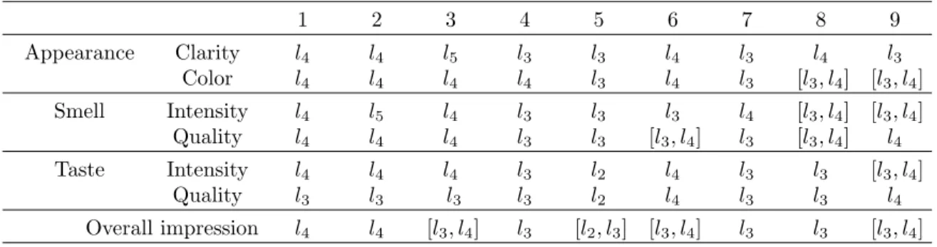
Nine wine experts recruited byAcademia Castellano Leonesa de Gastronom´ıa

y Alimentaci´on tasted eight red wines from Cigales Protected Designation of

Origin using the five linguistic terms of Table 1 (or the corresponding interval of

two consecutive linguistic terms, when they hesitated). The wines’ assessments

made by each expert are included in the Appendix.

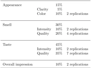
The nine experts assessed each wine taking into account the most important

sensory aspects in wine tasting: appearance, smell and taste, as well as essential

factors of each criterion, such as clarity, color, intensity and quality, and also

the overall impression (see Jackson [17]).

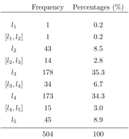
Table 2 contains the frequencies and percentages of the assessments in global

terms. Notice that the proportions ofl3andl4reached 69.6% of the assessments,

whilel1 and [l1, l2] only represented 0.4%. Also, it is important to remark that

eight out the nine experts used sometimes two consecutive terms, being this

type of the assessments 64 out of 504, i.e., approximately 12.7% of the cases.

Most tasting sheets, like Davis 20-point scorecard, use detailed score sheets

for evaluating sensory aspects of wines, giving a particular weight to each aspect

in the total score (see Jackson [17]). Since each sensory aspect may have different

importance in wine tasting, a weight was assigned to each criterion5_{. Aspects,}

l1 Insufficient

l2 Fair

l3 Good

l4 Very good

l5 Excellent

Table 1: Linguistic terms in L.

Frequency Percentages (%)

l1 1 0.2

[l1, l2] 1 0.2

l2 43 8.5

[l2, l3] 14 2.8

l3 178 35.3

[l3, l4] 34 6.7

l4 173 34.3

[l4, l5] 15 3.0

l5 45 8.9

504 100

Table 2: Summary of the assessments given by the wine experts.

weights and the corresponding replications considered in the case study are

shown in Table 3.

In order to know if the OQS used in the wine tasting was perceived as

uniform, after the wine tasting we asked the nine wine experts to complete an

on-line survey regarding the proximities between the terms of the OQS of Table

1.

With the information obtained in the survey, we generated the metrizable

OPM for each expert following the algorithm introduced in Garc´ıa-Lapresta et

al. [9, 2.3]. This algorithm starts by asking the expert about the comparison

between the ordinal proximities π12 and π23. The next question differs

de-pending on whether one of these ordinal degrees of proximity is greater than

the other or they are the same. The algorithm continues with similar questions

Appearance 15%

Clarity 5%

Color 10% 2 replications

Smell 30%

Intensity 10% 2 replications

Quality 20% 4 replications

Taste 45%

Intensity 10% 2 replications

Quality 35% 7 replications

Overall impression 10% 2 replications

Table 3: Sensory aspects and replications.

comparing the ordinal proximities between the remaining pairs of terms of the

OQS until the metrizable OPM is obtained.

The matrices associated with the metrizable OPMs of the nine experts were

A3223=        

δ1 δ3 δ5 δ6 δ7

δ1 δ2 δ4 δ6

δ1 δ2 δ5

δ1 δ3

δ1        

, A3234=        

δ1 δ3 δ5 δ7 δ9

δ1 δ2 δ5 δ8

δ1 δ3 δ6

δ1 δ4

δ1         ,

A3342=        

δ1 δ3 δ5 δ8 δ9

δ1 δ3 δ6 δ7

δ1 δ4 δ5

δ1 δ2

δ1        

, A3432=        

δ1 δ3 δ5 δ7 δ8

δ1 δ4 δ5 δ6

δ1 δ3 δ4

δ1 δ2

A0₃₄₃₂=



      

δ1 δ3 δ6 δ8 δ9

δ1 δ4 δ6 δ7

δ1 δ3 δ5

δ1 δ2

δ1 

      

.

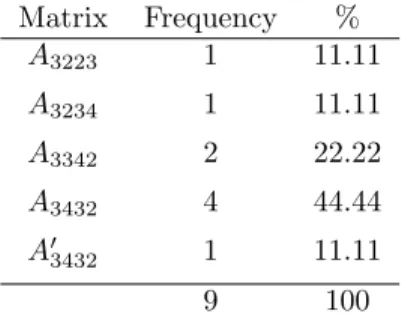
The frequency of these matrices is shown in Table 4. It is interesting to note

that none of the experts perceived the OQS as uniform.

Matrix Frequency %

A3223 1 11.11

A3234 1 11.11

A3342 2 22.22

A3432 4 44.44

A0₃₄₃₂ 1 11.11

9 100

Table 4: Matrices of the survey.

Since experts’ opinions about the proximities between the linguistic terms

of the OQS produced 5 different metrizable OPMs, it was advisable to find

a collective metrizable OPM that represents individual opinions as faithfully

as possible. To do that, we applied the aggregation procedure introduced in

Garc´ıa-Lapresta et al. [9, 4.3]. The procedure is based on weighted-metrics and

it provides the metrizable OPM that minimizes the sum of distances (square

distances) between itself and the metrizable OPMs of the experts.

The final outcome obtained after applying the mentioned aggregation

pro-cedure was the metrizable OPM associated with the proximity matrix A3432

that can be visualized in Fig. 2.

l1 l2 l3 l4 l5

Figure 2: Metrizable OPM with associated matrix A3432.

Once the metrizable OPM was obtained, we generated the extension of π

considers the proximities between the assessments given by agents andlg. Thus, we considered the pairs of δ’s contained in the last column of the proximity matrix associated withπ∗:

                 

π∗(l1, l5)

π∗([l1, l2], l5)

π∗(l2, l5)

π∗_([l

2, l3], l5)

π∗(l3, l5)

π∗([l3, l4], l5)

π∗(l4, l5)

π∗([l4, l5], l5)

π∗(l5, l5)                   =                  

(δ8, δ8)

(δ6, δ8)

(δ6, δ6)

(δ4, δ6)

(δ4, δ4)

(δ2, δ4)

(δ2, δ2)

(δ1, δ2)

(δ1, δ1)                   . (2)

After replicating the profiles according to Table 3 and applying the steps 3,

4, 5 and 6, we obtain the following pairs of medians:

M1=M3=M5=M6=M7= (δ4, δ4),(δ4, δ4)

,

M2=M8= (δ2, δ4),(δ2, δ4)

, M4= (δ2, δ2),(δ2, δ2)

.

Then, M4 4 (M2 ∼4 M8) 4 (M1 ∼4 M3 ∼4 M5 ∼4 M6 ∼4 M7).

In order to break the ties between wines 2 and 8, and wines 1, 3, 5, 6 and 7,

it is necessary to use the tie-breaking procedure of step 7.

For wines 2 and 8, after two tiebreakers, we have:

M2= (δ2, δ4),(δ4, δ4)

, M8= (δ2, δ4),(δ2, δ4)

.

Then, M4 4 M8 4 M2 4 (M1 ∼4 M3 ∼4 M5 ∼4 M6 ∼4 M7).

For wines 1, 3, 5, 6 and 7, after applying a tiebreaker, we have:

M1= (δ2, δ4),(δ4, δ4)

, M3=M5=M6=M7= (δ4, δ4),(δ4, δ4)

.

Then, M4 4 M8 4 M2 4 M1 4 (M5 ∼4 M3 ∼4 M6 ∼4 M7).

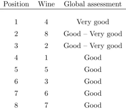
After applying again the tie-breaking procedure for the rest of wines, we

finally obtain the following ranking:

M4 4 M8 4 M2 4 M1 4 M5 4 M3 4 M6 4 M7.

Table 5 contains the final ranking of wines and the global assessment

Position Wine Global assessment

1 4 Very good

2 8 Good – Very good

3 2 Good – Very good

4 1 Good

5 5 Good

6 3 Good

7 6 Good

8 7 Good

Table 5: Ranking of wines obtained after applying the MCDM procedure.

obtained taking into account the initial pairs of ordinal degrees of proximity for

each wine and the last column of the proximity matrix associated withπ∗ (Eq. (2)).

For instance, for wine 2 the initial pair of medians is M2= (δ2, δ4),(δ2, δ4),

which correspond to [l3, l4] inπ∗. Thus, the global assessment for the wine 2 is

between Good and Very good.

5. Concluding remarks

Since words are more appropriate than numbers for expressing human

sub-jective opinions, many decision-making problems use ordered qualitative scales

formed by linguistic terms for evaluating alternatives.

In general, the use of ordered qualitative scales is based on the implicit

assumption that scales are uniform, assigning a numerical value to each linguistic

term of the scale. However, sometimes agents can perceive that the proximities

between the terms of the scale are not identical. In these cases, the conversion of

linguistic terms into numerical values is meaningless, being more appropriate an

ordinal approach for dealing with these non-uniform ordered qualitative scales.

In this paper, we have introduced a MCDM procedure that is based on

the ordinal proximities between the highest linguistic term of the scale and the

individual assessments (a single term or two consecutive linguistic terms of the

scale, when they hesitate).

It is worth pointing out that our proposal avoids the use of numerical values

criteria are used in a qualitative fashion by replicating experts’ opinions

pro-portionally to the weights.

Section 4 illustrated the practicality of the procedure in a wine tasting where

experts assessed eight wines regarding different criteria. However, our procedure

can be implemented in many different scenarios such as satisfaction surveys,

quality of life questionnaires, or quality controls in manufacturing processes,

when agents evaluate a set of alternatives using the same ordered qualitative

scale for each criterion.

For further research, it could be interesting to devise a MCDM procedure

that considers different ordered qualitative scales (equipped with the

corre-sponding ordinal proximity measures) associated with the criteria.

Acknowledgments.

The authors are grateful to Academia Castellano Leonesa de Gastronom´ıa

y Alimentaci´on andConsejo Regulador de la Denominaci´on de Origen Cigales,

specially to his president, Julio Valles, to the nine wine experts for their

col-laboration in the wine tasting, and also to three anonymous referees for their

useful comments and suggestions. The financial support of the Spanish

Minis-terio de Econom´ıa y Competitividad (project ECO2016-77900-P) and ERDF is

acknowledged.

References

[1] Balinski, M., Laraki, R.: A theory of measuring, electing and ranking.

Proceedings of the National Academy of Sciences of the United States of

America 104, pp. 8720-8725, 2007.

[2] Balinski, M., Laraki, R.: Majority Judgment: Measuring, Ranking, and

Electing. The MIT Press, Cambridge, MA, 2011.

[3] Balinski, M., Laraki, R.: How best to rank wines: Majority Judgment,

in: Wine Economics: Quantitative Studies and Empirical Observations.

Palgrave-MacMillan, pp. 149-172, 2013.

[4] Bustince, H., Fern´andez, J., Koles´arov´a, A., Mesiar, R.: Generation of

linear orders for intervals by means of aggregation functions. Fuzzy Sets

[5] Falc´o, E., Garc´ıa-Lapresta, J.L., Rosell´o, L.: Allowing agents to be

impre-cise: A proposal using multiple linguistic terms. Information Sciences 258,

pp. 249-265, 2014.

[6] Fasolo, B., Bana e Costa, C.A.: Tailoring value elicitation to decision

makers’ numeracy and fluency: Expressing value judgments in numbers

or words. Omega 44, pp. 83-90, 2014.

[7] Franceschini, F. , Galetto, M., Varetto, M.: Qualitative ordinal scales: the

concept of ordinal range. Quality Engineering 16, pp. 515-524, 2004.

[8] Garc´ıa-Lapresta, J.L., Gonz´alez del Pozo, R.: An ordinal multi-criteria

decision-making procedure in the context of uniform qualitative scales, in:

Soft Computing Applications for Group Decision-making and Consensus

Modeling (eds. M. Collan, J. Kacprzyk). Studies in Fuzziness and Soft

Computing 357. Springer, pp. 297-304, 2018.

[9] Garc´ıa-Lapresta, J.L., Gonz´alez del Pozo, R., P´erez-Rom´an, D.: Metrizable

ordinal proximity measures and their aggregation. Information Sciences

448-449, pp. 149-163, 2018.

[10] Garc´ıa-Lapresta, J.L., P´erez-Rom´an, D.: Ordinal proximity measures in

the context of unbalanced qualitative scales and some applications to

con-sensus and clustering. Applied Soft Computing 35, pp. 864-872, 2015.

[11] Garc´ıa-Lapresta, J.L., P´erez-Rom´an, D.: A consensus reaching process in

the context of non-uniform ordered qualitative scales. Fuzzy Optimization

and Decision Making 16, pp. 449-461, 2017.

[12] Garc´ıa-Lapresta, J.L., P´erez-Rom´an, D.: Aggregating opinions in

non-uniform ordered qualitative scales. Applied Soft Computing 67, pp.

652-657, 2018.

[13] Greco, S., Ehrgott, M., Figueira, J.R. (Eds.): Multiple Criteria Decision

Analysis: State of the Art Surveys. International Series in Operations

Re-search & Management Science 233, Springer, 2016.

[14] Herrera, F., Herrera-Viedma, E., Mart´ınez, L.: A fuzzy linguistic

method-ology to deal with unbalanced linguistic term sets. IEEE Transactions on

[15] Herrera-Viedma, E., L´opez-Herrera, A.G.: A model of an information

re-trieval system with unbalanced fuzzy linguistic information. International

Journal of Intelligent Systems 22, pp. 1197-1214, 2007.

[16] Hong-Bin, Y., Tieju, M., Van-Nam, H.: On qualitative multi-attribute

group decision making and its consensus measure: A probability based

perspective. Omega 70, pp. 94-117, 2017.

[17] Jackson, R.S.: Wine Tasting: A Professional Handbook. Elsevier Academic

Press, 2017.

[18] Koles´arov´a, A., Mayor, G., Mesiar, R.: Weighted ordinal means.

Informa-tion Sciences 177, pp. 3822-3830, 2007.

[19] Larichev, O., Brown, R.: Numerical and verbal decision analysis:

compar-ison on practical cases. Journal of Multi-Criteria Decision Analysis 9, pp.

263-274, 2000.

[20] Likert, R.: A technique for the measurement of attitudes. Archives of

Psy-chology 22 (140), pp. 1-55, 1932.

[21] Lozano, L.M, Garc´ıa-Cueto, E., Mu˜niz, J.: Effect of the number of response

categories on the reliability and validity of rating scales. European Journal

of Research Methods for the Behavioral and Social Sciences 4, pp. 73-79,

2008.

[22] Miller, G.A.: The magical number seven, plus or minus two: some limits

on our capacity for processing information. Psychological Review, 63(2),

pp. 81-97, 1956.

[23] Roberts, F.S.: Measurement Theory. Addison-Wesley Publishing Company,

Reading, 1979.

[24] Teigen, K.H.: The language of uncertainty. Acta Psychologica 68, pp.

27-38, 1988.

[25] Trav´e-Massuy`es, L., Piera, N.: The orders of magnitude models as

quali-tative algebras. Proceedings of the 11th International Joint Conference on

Artificial Intelligence 2, pp. 1261-1266, 1989.

[26] Windschitl, P.D., Wells, G.L.: Measuring psychological uncertainty: Verbal

versus numeric methods. Journal of Experimental Psychology: Applied 2,

[27] Xu, Z.S., Yager, R.R.: Some geometric aggregation operators based on

intuitionistic fuzzy sets. International Journal of General Systems 8, pp.

417-433, 2006.

[28] Zadeh, L.A.: The concept of a linguistic variable and its application to

approximate reasoning. Information Sciences 8, pp. 301-357, 1978.

[29] Zimmer, A.C.: Verbal vs. numerical processing of subjective probabilities.

Appendix

1 2 3 4 5 6 7 8 9

Appearance Clarity l4 l4 l5 l3 l3 l4 l3 l4 l3

Color l4 l4 l4 l4 l3 l4 l3 [l3, l4] [l3, l4]

Smell Intensity l4 l5 l4 l3 l3 l3 l4 [l3, l4] [l3, l4]

Quality l4 l4 l4 l3 l3 [l3, l4] l3 [l3, l4] l4

Taste Intensity l4 l4 l4 l3 l2 l4 l3 l3 [l3, l4]

Quality l3 l3 l3 l3 l2 l4 l3 l3 l4

Overall impression l4 l4 [l3, l4] l3 [l2, l3] [l3, l4] l3 l3 [l3, l4]

Table 6: Assessments obtained for wine 1.

1 2 3 4 5 6 7 8 9

Appearance Clarity l5 l4 l5 l5 l3 l4 l3 l4 l4

Color l4 l4 l4 l4 l4 l2 l3 l3 l4

Smell Intensity l4 l4 l3 l4 [l2, l3] l3 l4 [l3, l4] l3

Quality [l4, l5] l3 l4 l4 l3 l3 l3 l3 l3

Taste Intensity l4 [l3, l4] l4 l3 l3 l3 l2 l4 l3

Quality l4 [l3, l4] l4 l3 l2 l2 l2 l4 l4

Overall impression l4 l3 [l3, l4] l4 l2 l3 [l2, l3] [l3, l4] l3

1 2 3 4 5 6 7 8 9

Appearance Clarity l5 l4 l4 l5 l4 l4 l4 l4 l3

Color l5 l4 l3 l5 l4 l3 l4 l4 l4

Smell Intensity l4 l4 l4 l3 l4 l3 l4 l4 l4

Quality l2 l2 l3 l3 l3 l2 l3 l4 [l3, l4]

Taste Intensity l2 l3 l4 l3 l3 l3 l4 l4 l4

Quality l1 l2 l3 l4 l3 [l2, l3] l3 l4 [l3, l4]

Overall impression l2 l2 l3 l4 [l3, l4] [l2, l3] [l3, l4] l4 [l3, l4]

Table 8: Assessments obtained for wine 3.

1 2 3 4 5 6 7 8 9

Appearance Clarity l5 l4 l5 l4 l4 l4 l4 l4 [l3, l4]

Color l5 l5 l4 l5 l4 l4 l4 l4 [l3, l4]

Smell Intensity l5 l5 l4 l5 l4 l5 l3 [l4, l5] [l3, l4]

Quality l5 l4 l3 l4 l3 l5 l3 l4 l3

Taste Intensity l5 l4 l4 l5 l3 l4 l3 l4 l4

Quality l5 l3 [l3, l4] l4 l3 l4 l3 [l3, l4] [l4, l5]

Overall impression l5 l4 l4 l5 l3 l4 l3 l4 l4

Table 9: Assessments obtained for wine 4.

1 2 3 4 5 6 7 8 9

Appearance Clarity l5 l4 l4 l3 l4 [l3, l4] l4 l4 [l4, l5]

Color l5 l5 l4 l3 l4 l3 l4 l4 l4

Smell Intensity l3 l5 l3 l3 l4 l3 l4 l4 l3

Quality l3 l5 l2 l3 l3 l4 l3 [l3, l4] [l3, l4]

Taste Intensity l4 l4 l4 l2 l3 l3 l2 l4 l4

Quality l3 [l4, l5] l3 l2 l2 l3 l3 l4 l4

Overall impression l3 [l4, l5] l3 l3 l3 l3 [l3, l4] l4 l4

Table 10: Assessments obtained for wine 5.

1 2 3 4 5 6 7 8 9

Appearance Clarity l5 l4 l5 l4 l4 l3 l3 l4 [l4, l5]

Color l5 [l2, l3] l3 l3 l4 l3 l3 l3 [l3, l4]

Smell Intensity l3 l3 l3 l2 l3 l4 l4 l3 l3

Quality l2 l4 l3 l3 l2 l4 l3 l3 l3

Taste Intensity l3 l3 l3 l4 l3 l4 l2 l3 l3

Quality l3 l2 l3 l3 l3 l3 l3 l3 l3

Overall impression l3 l2 l3 l3 l3 [l3, l4] l3 l3 l3

1 2 3 4 5 6 7 8 9

Appearance Clarity l5 l3 l5 l4 l3 l2 l3 l4 l3

Color l5 l4 l4 l3 l3 l3 l3 l4 l3

Smell Intensity l4 [l4, l5] l3 l2 l3 l2 l2 [l4, l5] l4

Quality l4 l3 l2 l2 l2 l2 l3 [l4, l5] l4

Taste Intensity l5 l4 l3 l3 l3 l3 l2 [l4, l5] [l2, l3]

Quality [l4, l5] l3 l3 l3 l2 l2 l2 l4 [l2, l3]

Overall impression [l4, l5] l3 [l2, l3] l3 [l2, l3] l2 [l2, l3] l4 [l2, l3]

Table 12: Assessments obtained for wine 7.

1 2 3 4 5 6 7 8 9

Appearance Clarity l5 l3 l5 l5 l4 l3 l4 l4 l4

Color l5 [l4, l5] l3 l5 l4 l3 l3 [l3, l4] [l4, l5]

Smell Intensity l5 l4 l3 l4 l3 l3 l3 l3 l4

Quality l4 l4 l3 l5 l3 [l1, l2] l3 l3 [l3, l4]

Taste Intensity l4 l4 l4 l4 l2 l3 l2 l4 l4

Quality l4 l3 l3 l4 l2 l3 l2 l4 l4

Overall impression l4 l4 l3 l5 [l2, l3] l3 [l2, l3] [l3, l4] l4