Bézier variant of modified Srivastava–Gupta operators

Published online: April 5, 2017

B ´EZIER VARIANT OF MODIFIED SRIVASTAVA–GUPTA

OPERATORS

TRAPTI NEER, NURHAYAT ISPIR, AND PURSHOTTAM NARAIN AGRAWAL

Abstract. Srivastava and Gupta proposed in 2003 a general family of linear positive operators which include several well known operators as its special cases and investigated the rate of convergence of these operators for functions of bounded variation by using the decomposition techniques. Subsequently, researchers proposed several modifications of these operators and studied their various approximation properties. Yadav, in 2014, proposed a modification of these operators and studied a Voronovskaya-type approximation theorem and statistical convergence. In this paper, we introduce the B´ezier variant of the operators defined by Yadav and give a direct approximation theorem by means of the Ditzian–Totik modulus of smoothness and the rate of convergence for absolutely continuous functions having a derivative equivalent to a function of bounded variation. Furthermore, we show the comparisons of the rate of convergence of the Srivastava–Gupta operators vis-`a-vis its B´ezier variant to a certain function by illustrative graphics using Maple algorithms.

1. _Introduction

In order to approximate Lebesgue integrable functions on [0,∞), Gupta and Srivastava [14] introduced a general family of summation-integral type operators as

Ln,c(f, x) =n

∞ X

k=1

pn,k(x, c)

Z ∞ 0

pn+c,k−1(t, c)f(t)dt+pn,0(x, c)f(0), (1.1)

where

pn,k(x, c) = (−x)k

k! φ

(k)

n,c(x)

and

φn,c(x) =

(

e−nx, c= 0, (1 +cx)−n/c_{, c∈}

N:={1,2,3, . . .}.

2010Mathematics Subject Classification. 41A25, 47A48.

Key words and phrases. B´ezier operators, Gupta–Srivastava operators, Ditzian–Totik modulus of smoothness, rate of convergence, bounded variation.

Ispir and Yuksel [11] introduced the B´ezier variant of the operators (1.1) and stud-ied the estimate of the rate of convergence of these operators for functions of bounded variation. Verma and Agrawal [15] introduced the generalized form of the operators (1.1) and studied some of its approximation properties. Deo [6] gave a modification of these operators and established the rate of convergence and Voronovskaya-type result. Recently, Acar et al. [1] introduced a Stancu-type generalization of the operators (1.1) and obtained an estimate of the rate of con-vergence for functions having derivatives of bounded variation and also studied the simultaneous approximation for these operators.

Yadav [16] introduced a modification of the operators (1.1) as

Gn,c(f, x) =n

∞ X

k=1

pn,k(x, c)

Z ∞ 0

pn+c,k−1(t, c)f

_(n−c)t

n

dt

+pn,0(x, c)f(0).

(1.2)

and studied its moment estimates, direct estimate, asymptotic formula and statisti-cal convergence. Very recently, Maheshwari [13] studied the rate of approximation for the functions having derivative of bounded variation on every finite subinterval of [0,∞) for the operators (1.2).

It is well known that B´ezier curves are the parametric curves used in computer graphics and designs. In vector graphics they are used to model smooth curves and also used in animation designs. Zeng and Piriou [18] pioneered the study of B´ezier variants of Bernstein operators. The papers by other researchers (e.g., [3, 5, 8, 13, 17]) motivate us to study further in this direction.

The present paper is an attempt to continue the study of B´ezier variants of different sequences of operators. We propose a B´ezier variant of the operators given by (1.2) as

Gα_n,c(f, x) =n

∞ X

k=1

Q(_n,kα)(x, c)

Z ∞ 0

pn+c,k−1(t, c)f _(n

−c)t n

dt

+Q(_n,α₀)(x, c)f(0),

(1.3)

whereQ(_n,kα)(x, c) = [Jn,k(x, c)] α

−[Jn,k+1(x, c)]

α

,α≥1, withJn,k(x, c) =

P∞

The aim of this paper is to investigate a direct approximation result and the rate of convergence for functions having a derivative equivalent with a function of bounded variation on every finite subinterval of [0,∞) for the operators (1.2). Lastly, a comparison of the rate of convergence of the operators (1.2) vis-`a-vis operators (1.3) to a certain function is illustrated by some graphics.

2. Auxiliary results

Lemma 2.1([16]). ForGn,c(tm, x),m= 0,1,2, one has (1) Gn,c(1, x) = 1

(2) Gn,c(t, x) =x

(3) Gn,c(t2_{, x) =} (n−c)(x2(n+c)+2x)

n(n−2c) .

Consequently,

Gn,c((t−x)2, x) =x

2_{c(2n−c) + 2(n−c)x}

n(n−2c) and

Gn,c((t−x)2, x)≤ λx(1 +cx)

n for sufficiently largenandλ >1. From [13], one has

Gn,c((t−x)2r, x) =O(n−r). (2.1) Remark 2.2. We have

Gαn,c(1;x) =

∞ X

k=0

Q(_n,kα)(x, c) = [Jn,0(x, c)]

α

=



 ∞ X

j=0

pn,k(x, c)





α

= 1,

sinceP∞_j=0pn,k(x, c) = 1.

LetCB[0,∞) denote the space of all bounded and continuous functions on [0,∞) endowed with the norm

kfk= sup

[0,∞) |f(x)|.

Lemma 2.3. For everyf ∈CB[0,∞), we have

kGα_n,c(f;.)k ≤ kfk.

Applying Remark 2.2, the proof of this lemma easily follows. Hence the details are omitted.

Remark 2.4. For 0≤a, b≤1,α≥1, using the inequality

|aα−bα| ≤α|a−b|

and from the definition ofQ(_n,kα)(x, c), for allk= 0,1,2, . . ., we have

Hence from the definition ofGα

n,c(f;x) we get

|Gαn,c(f, x)| ≤αGn,c(|f|, x).

3. _{Main results}

To describe our first result, we recall the definitions of the Ditzian–Totik first order modulus of smoothness and theK-functional [7]. Letφ(x) =px(1 +cx), f ∈

C[0,∞). The first order modulus of smoothness is given by

ωφ(f, t) = sup

0<h≤t

f

x+hφ(x) 2

−f

x−hφ(x)

2

, x±hφ(x)

2 ∈[0,∞)

,

and the appropriate Petree’sK-functional is defined by

Kφ(f, t) = inf g∈Wφ

{kf−gk+tkφg0k+t2kg0k, t >0}, (3.1) where Wφ ={g :g ∈ACloc,kφg0k <∞,kg0k <∞} and g ∈ACloc means thatg is an absolutely continuous function on every [a, b]⊂[0,∞). It is well known ([7] Theorem 3.1.2) thatKφ(f, t)∼ωφ(f, t), which means that there exists a constant C >0 such that

C−1ωφ(f, t)≤Kφ(f, t)≤Cωφ(f, t). (3.2) Now, we establish a direct approximation theorem by means of the Ditzian–Totik modulus of smoothness.

Theorem 3.1. Letf ∈C[0,∞)andφ(x) =px(1 +cx), then for everyx∈[0,∞), we have

|Gα_n,c(f;x)−f(x)| ≤Cωφ

f;√1

n

, (3.3)

whereC is a constant independent ofn andx.

Proof. For fixednandx, choosingg=gn,x∈Wφ and using the representation

g(t) =g(x) +

Z t

x

g0(u)du,

we get

|Gα_n,c(g;x)−g(x)|=

Gα_n,c

Z t

x

g0(u)du;x

. (3.4)

Now to find the estimate we split the domain into two parts: Fnc = [0,1n] and Fn= (_n1,∞). First, ifx∈(_n1,∞) thenGα

n,c((t−x)2;x)∼

2α nφ

2_(x).

We have

Z t

x

g0(u)du

≤ kφg0k

Z t

x 1 φ(u)du

For anyx, t∈(0,∞), we find that Z t x 1 φ(u)du = Z t x 1 p

u(1 +cu)du

≤ Z t x 1 √ u+ 1 √

1 +cu

du ≤2 √

t−√x+

√

1 +ct−√1 +cx c

= 2|t−x|

1

√

t+√x+

1

√

1 +ct+√1 +cx

<2|t−x| 1 √ x+ 1 √

1 +cx

≤_p2(c+ 1)

c(c−1)

|t−x|

φ(x) .

(3.6)

Combining (3.4)-(3.6) and using the Cauchy–Schwarz inequality, we obtain

|Gα_n,c(g;x)−g(x)|<_p2(c+ 1) c(c−1)kφg

0_kφ−1_(x)Gα

n,c(|t−x|;x)

≤_p2(c+ 1)

c(c−1)kφg

0_kφ−1_(x)Gα

n,c((t−x)

2_;x) 1/2

≤_p2(c+ 1)

c(c−1)kφg

0_k

2α n

1/2

≤Ckφg0k√1

n.

(3.7)

Forx∈Fc

n= [0,1/n],Gαn,c((t−x)2;x)∼2nα2 and

Z t x

g0(u)du

≤ kg0k |t−x|.

Therefore, using the Cauchy–Schwarz inequality we have

|Gα_n,c(g;x)−g(x)| ≤ kg0kGα_n,c(|t−x|;x)

≤ kg0k

Gα_n,c((t−x)2;x)

1/2

≤ kg0k √

2α n ≤Ckg

0_k1

n.

(3.8)

From (3.7) and (3.8), we obtain

|Gα_n,c(g;x)−g(x)|< C

kφg0k√1

n+kg

0_k1

n

Using Lemma 2.3 and (3.9), we can write

|Gα_n,c(f;x)−f(x)| ≤ |Gα_n,c(f −g;x)|+|f(x)−g(x)|+|Gα_n,c(g;x)−g(x)|

≤C

kf−gk+kφg0k√1

n +kg

0_k1

n

. (3.10)

Taking the infimum on the right hand side of the above inequality over allg∈Wφ, we get

|Gα_n,c(f;x)−f(x)|=CKφ

f;√1

n

.

Using Kφ(f, t) ∼ωφ(f, t) and (3.2), we get the desired relation (3.3). This

com-pletes the proof of the theorem.

Lastly, we shall discuss the rate of approximation of functions with a derivative of bounded variation on [0,∞). Let DBVγ[0,∞), γ ≥ 0, denote the class of all absolutely continuous functionsf defined on [0,∞), having a derivativef0 equiva-lent with a function of bounded variation on every finite subinterval of [0,∞) and

|f(t)| ≤M tγ_.

We observe that the functionsf ∈DBVγ[0,∞) possess a representation

f(x) =

Z x

0

g(t)dt+f(0),

where g ∈ BV[0,∞), i.e., g is a function of bounded variation on every finite subinterval of [0,∞).

In order to discuss the approximation of functions with derivatives of bounded variation, we express the operatorsGα

n,c in an integral form as follows:

Gα_n,c(f;x) =

Z ∞ 0

K_n,cα (x, t)f

_(n −c)t

n

dt, (3.11)

where the kernelKn,cα (x, t) is given by

Kn,cα (x, t) =

∞ X

k=1

Q(_n,kα)(x, c)pn+c,k−1(t, c) +Q(n,α0)(x, c)δ(t),

δ(u) being the Dirac delta function.

Lemma 3.2. For a fixedx∈(0,∞)and sufficiently large n, we have (1) ξα

n,c(x, y) =

Ry 0 K

α

n,c(x, t)dt≤α

λx(1+cx)

n

1

(x−y)2, 0≤y < x,

(2) 1−ξα

n,c(x, z) =

R∞

z K

α

n,c(x, t)dt≤α

λx(1+cx)

n

1

Proof. (1) Using Lemma 2.1 and Remark 2.4, we get

ξ_n,cα (x, y) = y

Z

0

K_n,cα (x, t)dt≤ Z y

0

_x−t

x−y

2

K_n,cα (x, t)dt

≤Gα_n,c((t−x)2;x)(x−y)−2

≤αGn,c((t−x)2;x)(x−y)−2

≤λαx(1 +cx)

n

1 (x−y)2.

The proof of (2) is similar, hence the details are omitted.

Theorem 3.3. Let f ∈DBVγ[0,∞). Then, for every x∈(0,∞)and sufficiently largen, we have

|Gα_n,c(f;x)−f(x)| ≤ 1

α+ 1|f

0_{(x+) +αf}0_(x−)| r

2αx(1 +cx) n

+ α

α+ 1|f

0_(x+)−f0_(x−)| r

2αx(1 +cx) n

+λα(1 +cx) n

[√n] X

k=1

x+x/k

_

x−x/k

f_x0 +√x

n x+x/√n

_

x−x/√n f_x0

+λα(1 +cx)

nx |f(2x)−f(x)−xf

0_(x+)|

+αC(n, c, r, x)

nr +

|f(x)|

x

λα(1 +cx)

n ,

whereWb

af(x)denotes the total variation of f(x)on [a, b]andf

0

x is defined by

fx0(t) =

  

 

f0(t)−f0(x−), 0≤t < x

0, t=x

f0(t)−f0(x+), x < t <∞.

(3.12)

Proof. SinceGα

n,c(1;x) = 1, using (3.11), for everyx∈(0,∞) we get Gαn,c(t;x)−f(x) =

Z ∞ 0

Kn,cα (x, t)(f(t)−f(x))dt

=

Z ∞ 0

K_n,cα (x, t)

Z t

x

f0(u)du dt.

(3.13)

For any f ∈DBVγ[0,∞), from (3.12) we may write

f0(u) =f_x0(u) + 1 α+ 1(f

0_{(x+) +αf}0_(x−))

+1 2(f

0_(x+)−f0_{(x−))sgn(u−x) +}α−1

α+ 1

×δx(u)[f0(u)−1

2(f

0_{(x+) +f}0_(x−))],

where

δx(u) =

(

1, u=x 0, u6=x.

From equations (3.13) and (3.14), we get

Gα_n,c(t;x)−f(x) =

Z ∞

0

K_n,cα (x, t)

Z t

x

f_x0(u) + 1 α+ 1(f

0_{(x+) +αf}0_(x−))

+1 2(f

0_(x+)−f0_(x−))

sgn(u−x) +α−1 α+ 1

+δx(u)f0(u)−1

2(f

0_{(x+) +f}0_(x−))

du

dt

=A1+A2+A3+Aαn,c(f

0

x, x) +B α n,c(f

0

x, x),

where

A1= Z ∞

0 Z t

x 1 α+ 1(f

0_{(x+) +αf}0_(x−))du

K_n,cα (x, t)dt,

A2= Z ∞

0

K_n,cα (x, t)

Z t

x 1 2(f

0_(x+)−f0_{(x−))sgn(u−x) +}α−1

α+ 1

du

dt,

A3= Z ∞

0 Z t

x

f0(u)−1

2(f

0_{(x+) +f}0_(x−))

δx(u)du

K_n,cα (x, t)dt,

Aα_n,c(f_x0, x) =

Z x

0 Z t

x

f_x0(u)du

K_n,cα (x, t)dt,

B_n,cα (f_x0, x) =

Z ∞

x

Z t

x

f_x0(u)du

K_n,cα (x, t)dt.

Obviously,

A3= Z ∞

0 Z t

x

f0(u)−1

2(f

0_{(x+) +f}0_(x−))

δx(u)du

K_n,cα (x, t)dt

= 0.

(3.15)

We get

A1= Z ∞

0 Z t

x 1 α+ 1(f

0_{(x+) +αf}0_(x−))duKα

n,c(x, t)dt

= 1

α+ 1(f

0_{(x+) +αf}0_(x−))Z ∞

0

(t−x)K_n,cα (x, t)dt

= 1

α+ 1(f

0_{(x+) +αf}0_(x−))Gα

n,c((t−x);x)

and

A2= Z ∞

0

K_n,cα (x, t)

Z t

x 1 2(f

0_(x+)−f0_(x−))

sgn(u−x) +α−1 α+ 1

du dt = 1 2

f0(x+)−f0(x−)

− Z x 0 Z x t

sgn(u−x) +α−1 α+ 1

du

K_n,cα dt

+ Z ∞ x Zt x

sgn(u−x) +α−1 α+ 1

du

Kn,cα (x, t)dt

≤ α

α+ 1

f0(x+)−f0(x−)

Z ∞

0

|t−x|Kn,cα (x, t)dt

= α

α+ 1

f0(x+)−f0(x−)

Gα_n,c

|t−x|;x

.

(3.17)

Using Lemma 2.4 and equations (3.13–3.17) and applying the Cauchy–Schwarz inequality we obtain

|Gα_n,c(f;x)−f(x)| ≤ 1

α+ 1|f

0_{(x+) +αf}0_(x−)|(αG

n,c((t−x)2;x))1/2

+ α

α+ 1|f

0_(x+)−f0_(x−)|(αG

n,c((t−x)2;x))1/2 +|Aα_n,c(f_x0, x)|+|B_n,cα (f_x0, x)|

≤ 1

α+ 1|f

0_{(x+) +αf}0_(x−)| r

λαx(1 +cx) n

+ α

α+ 1|f

0_(x+)−f0_(x−)| r

λαx(1 +cx) n +|Aαn,c(fx0, x)|+|Bn,cα (fx0, x)|.

(3.18)

Thus our problem is reduced to calculate the estimates of the termsAα n,c(fx0, x) andB_n,cα (f_x0, x). SinceRb

a dtξ α

n,c(x, t)≤1 for all [a, b]⊆[0,∞), using integration by parts and applying Lemma 3.2 withy=x−x/√n, we have

|Aαn,c(fx0, x)|=

Z x 0 Z t x

fx0(u)du

dtξαn,c(x, t)

= Z x 0

ξαn,c(x, t)fx0(t)dt

≤ Z y 0

|f_x0(t)| |ξ_n,cα (x, t)|dt+

Z x

y

|f_x0(t)| |ξ_n,cα (x, t)|dt

≤λαx(1 +cx)

n Z y 0 x _ t

f_x0)(x−t)−2dt+

Z x

y x

_

t f_x0dt

≤λαx(1 +cx)

n Z y 0 x _ t

fx0(x−t)−2dt+ x

√

n x

_

x−x/√n fx0

=λαx(1 +cx) n

Z x−√x

n

0

x

_

t

fx0(x−t)−2dt+ x

√

n x

_

Substitutingu=x/(x−t), we get

λαx(1 +cx) n

Z x−x/ √

n

0

(x−t)−2 x

_

t

f_x0 dt= λαx(1 +cx)

n x −1Z √ n 1 x _

x−x/u f_x0 du

≤ λα(1 +cx)

n

[√n] X

k=1 Z k+1

k x

_

x−x/k f_x0du

≤ λ(1 +cx)

n

[√n] X

k=1

x

_

x−x/k fx0.

Thus,

|Aα_n,c(f_x0, x)| ≤ λ(1 +cx)

n

[√n] X

k=1

x

_

x−x/k

f_x0 +√x

n x

_

x−x/√n

f_x0. (3.19)

Again, using integration by parts in Bρ

n(fx0, x) and applying Lemma 3.2 and the Cauchy–Schwarz inequality, we have

|B_n,cα (f_x0, x)| ≤ Z ∞ 2x Z t x

f_x0(u)du

dtK_n,cα (x, t)

+

Z 2x

x

Z t

x

fx0(u)du

dt(1−ξαn,c(x, t))

≤ Z ∞ 2x

(f(t)−f(x))Kn,cα (x, t)

+|f0(x+)| Z ∞ 2x

(t−x)Kn,cα (x;t)dt

+

Z 2x

x

f_x0(u)du

|1−ξ_n,cα (x,2x)|+

Z 2x

x

f_x0(t)(1−ξ_n,cα (x, t))dt

≤ Z ∞ 2x

f(t)K_n,cα (x, t)

+|f(x)| Z ∞ 2x

K_n,cα (x, t)

+|f0(x+)| Z ∞

2x

(t−x)2K_n,cα (x;t)dt

1/2

+λα(1 +cx) nx

Z 2x

x

((f0(u)−f0(x+))du

+

Z x+x/ √

n

x

f_x0(t)dt

+λαx(1 +cx) n

Z 2x

x+x/√n

(t−x)−2f_x0(t)dt

.

We see that there exists an integerr(2r≥γ), such thatf(t) =O(t2r_{), ast→ ∞.} Now proceeding in a manner similar to the estimate ofAα

t=x+x u we get

|B_n,cα (f0, x)| ≤M

Z ∞ 2x

t2rK_n,cα (x, t)dt+|f(x)| Z ∞

2x

K_n,cα (x, t)dt

+|f0(x+)| r

λαx(1 +cx)

n +

λα(1 +cx)

nx |f(2x)−f(x)−xf

0_(x+)|

+√x

n x+x/√n

_

x

(f_x0) +λαx(1 +cx) n

Z 2x

x+x/√n

(t−x)−2f_x0(t)dt

≤M

Z ∞

2x

t2rK_n,cα (x, t)dt+|f(x)| Z ∞

2x

K_n,cα (x, t)dt

+|f0(x+)| r

λαx(1 +cx)

n +

λα(1 +cx)

nx |f(2x)−f(x)−xf

0_(x+)|

+√x

n x+x/√n

_

x

f_x0 +λα(1 +cx) n

[√n] X

k=1

x+x/√n

_

x

f_x0. (3.20)

For t ≥ 2x, we get t ≤ 2(t−x) and x ≤ t−x. Now using equation (2.1) and Lemma 3.2, we obtain

Z ∞ 2x

t2rK_n,cα (x, t)dt+|f(x)| Z ∞

2x

K_n,cα (x, t)dt

≤22r

Z ∞ 2x

(t−x)2rKn,cα (x, t)dt+

|f(x)|

x2 Z ∞

2x

(t−x)2Kn,cα (x, t)dt

≤ αC(n, c, r, x)

nr +

|f(x)|

x2

λαx(1 +cx)

n .

(3.21)

Collecting the estimates (3.18)–(3.21), we get the required result. This completes

the proof.

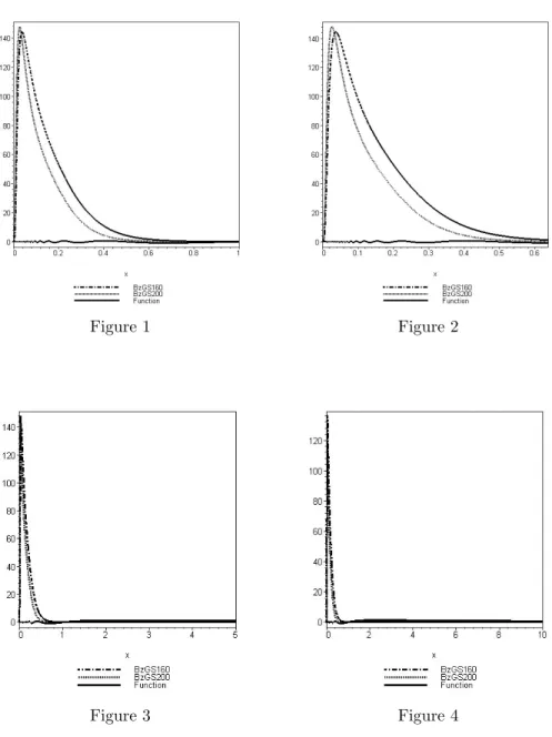
Next, we illustrate the comparison of the rate of convergence of the operators (1.2) and (1.3) to a certain function by some graphics using Maple algorithms.

Let us consider the function

f(x) =

(

0, x= 0

x1/3_{sin(π/x), x6= 0.} (3.22)

Then,f is of bounded variation on [0,1].

is given in Figures 1, 2, 3 and 4.

Figure 1 Figure 2

Figure 3 Figure 4

x∈[0,2/π] andx∈[0,10] is shown in Figures 5 and 6 respectively.

Figure 5 Figure 6

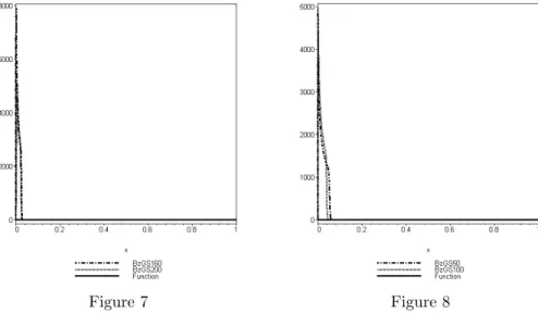
Example 3. In case c = 0, α= 10 forn = 160,n = 200 and n= 50, n = 100, the convergence of B´ezier–Gupta–Srivastava operators to the function f(x) given by (3.22) forx∈[0,1] is shown in Figures 7 and 8, respectively.

Figure 7 Figure 8

given by (3.22) is illustrated.

Figure 9

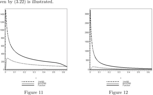
Now let us compare the convergence of the operatorsGn,cgiven by (1.2) andGα n,c given by (1.3)

In casec= 0, forn= 50 andα= 10, the comparison of the convergence of the operators (1.2) (named as Ydv in Figures) and the operators (1.3) to the function (3.22) is shown in Figure 10.

Figure 10

given by (3.22) is illustrated.

Figure 11 Figure 12

From the above comparisons, it turns out that the operator given by (1.3) yields a better rate of convergence than the operator given by (1.2) in certain cases.

References

[1] T. Acar, L. N. Mishra and V. N. Mishra, Simultaneous approximation for generalized Srivastava–Gupta operators, J. Funct. Spaces 2015, Article ID 936308, 11 pp. MR 3337423. [2] P. N. Agrawal, V. Gupta, A. Sathish Kumar and A. Kajla, Generalized Baskakov–Sz´asz type

operators, Appl. Math. Comput. 236 (2014), 311–324. MR 3197729.

[3] P. N. Agrawal, N. Ispir and A. Kajla, Approximation properties of Lupas-Kantorovich op-erators based on Polya distribution, Rend. Circ. Mat. Palermo (2) 65 (2016), 185–208. MR 3535450.

[4] R. Bojani´c and F. H. Chˆeng, Rate of convergence of Bernstein polynomials for functions with derivatives of bounded variation, J. Math. Anal. Appl. 141 (1989), 136–151. MR 1004589. [5] G. Chang, Generalized Bernstein-B´ezier polynomials, J. Comput. Math. 1 (1983), 322–327. [6] N. Deo, Faster rate of convergence on Srivastava–Gupta operators, Appl. Math. Comput. 218

(2012), 10486–10491. MR 2927065.

[7] Z. Ditzian and V. Totik, Moduli of smoothness, Springer-Verlag, New York, 1987. MR 0914149.

[8] S. S. Guo, G. F. Liu and Z. J. Song, Approximation by Bernstein–Durrmeyer–B´ezier operators inLpspaces, Acta Math. Sci. Ser. A Chin. Ed. 30 (2010), 1424–1434. MR 2789202. [9] N. Ispir, Rate of convergence of generalized rational type Baskakov operators, Math. Comput.

Modelling 46 (2007), 625–631. MR 2333526.

[10] N. Ispir, P. N. Agrawal and A. Kajla, Rate of convergence of Lupas Kantorovich operators based on Polya distribution, Appl. Math. Comput. 261 (2015), 323–329. MR 3345281. [11] N. Ispir and I. Yuksel, On the B´ezier variant of Srivastava–Gupta operators, Appl. Math.

E-Notes 5 (2005), 129–137. MR 2120140.

[12] H. Karsli, Rate of convergence of new Gamma type operators for functions with derivatives of bounded variation, Math. Comput. Modelling 45 (2007), 617–624. MR 2287309.

[14] H. M. Srivastava and V. Gupta, A certain family of summation-integral type operators, Math. Comput. Modelling 37 (2003), 1307–1315. MR 1996039.

[15] D. K. Verma and P. N. Agrawal, Convergence in simultaneous approximation for Srivastava– Gupta operators, Math. Sci. (Springer) 6 (2012), Art. 22, 8 pp. MR 3023672.

[16] R. Yadav, Approximation by modified Srivastava–Gupta operators, Appl. Math. Comput. 226 (2014), 61–66. MR 3144291.

[17] X.-M. Zeng, On the rate of convergence of two Bernstein–B´ezier type operators for bounded variation functions, II, J. Approx. Theory 104 (2000), 330–344. MR 1761905.

[18] X. Zeng and A. Piriou, On the rate of convergence of two Bernstein–B´ezier type operators for bounded variation functions. J. Approx. Theory 95 (1998), 369–387. MR 1657687.

T. NeerB

Department of Mathematics, Indian Institute of Technology Roorkee, Roorkee-247667, India triptineeriitr@gmail.com

N. Ispir

Department of Mathematics, Faculty of Sciences, Gazi University, 06500 Ankara, Turkey nispir@gazi.edu.tr

P. N. Agrawal

Department of Mathematics, Indian Institute of Technology Roorkee, Roorkee-247667, India pna iitr@yahoo.co.in