Maestría en Economía
Facultad de Ciencias Económicas
Universidad Nacional de La Plata
TESIS DE MAESTRIA
ALUMNO
Andrés Orlandi
TITULO
Dynamic Gains of Including Emerging Markets Assets in an International
Diversified Portfolios
DIRECTOR
Ricardo Bebczuk
FECHA DE DEFENSA
Dynamic Gains of Including Emerging Equity Market in an
International Diversified Portfolio
*Andres Orlandi
(December 2002)
Abstract
Using a utility based measure and under a conditional mean-variance framework this paper analyzes the economic value of diversifying into emerging market. Depending on risk tolerance characteristics, the value of diversifying into emerging equity markets is estimated to be between 100 and 300 annual basis points, even after imposing realistic constrains that investors face in these markets. Importantly, the methodology used in this paper allows studying how changes in the national and international environment affects this measure. The analysis indicate that while emerging market crises seem to reduce these economic gains, when US economy is in a recession, investing in emerging equity markets still help improving the portfolio performance. At the same time, although in the early nineties a capital market liberalization process took place, the gains of investing in emerging equities remain economically significant, with a growing trend from 2001 on.
*
1
Introduction
It is widely known in the asset allocation literature that when investors diversify
interna-tionally, significant performance gains can be obtained. Although this literature has been
concentrated in developed markets (De Santis and Gerard (1997)), from last decay
emerg-ing equity markets has gotten a lot of attention between academia and practitioners. Most
papers study whether adding emerging markets to benchmark portfolios statistically shifts
the mean variance frontier, using both conditional and unconditional information (DeSantis
(1994), Harvey (1994, 1995), Bekaert and Urias (1996), De Roon et al (2001), Li et al (2003)).
Once we know that emerging markets statistically improve the investment opportunity set,
a natural question that investors seek to answer is whether this new opportunity has any
economic value. In other words, it is interesting to get some idea about the value of
includ-ing equities from emerginclud-ing markets in an international diversified portfolio. In this paper I
address this issue, estimating the out-of-sample maximum fee that an investor is willing to
pay to switch from the ex-ante optimal portfolio of equities from developed economies, to the
ex-ante optimal portfolio including assets from both developed and developing countries1.
Importantly, I calculate the “ex-ante” certainty equivalent rate of return for the last two
decades in order to analyze the effect of the time-varying economic environment over this
measure of value across time.
Several authors analyze the roll of emerging equity markets in portfolio diversification
problems. Given the relatively low correlation between these equity markets and developed
ones, portfolio theory suggests that including holdings from these countries may improve the
portfolio performance. Taking this fact into account, DeSantis (1994) and Harvey (1995)
argue that US investors can benefit from including emerging markets asset in their portfolios
because emerging markets returns are not spanned by the developed ones. Similarfindings
can be found in Bekaert and Urias (1996). They argue that using emerging equity market
indices, previous studies do not consider the high transaction costs, low liquidity and
invest-ment constraints associated with investinvest-ment in emerging markets. Using closed-end country
funds, that is, funds that are available to international investors, they alsofind a diversifi
ca-tion benefit when including emerging equity markets in an international diversified portfolio.
On the other hand, De Roon et al (2001) suggest that when short-selling constraints are
included in the analysis (characteristic of emerging equity markets), the evidence in favor of
including developing markets equity holding tends to disappear. Nevertheless, their
statisti-cal analysis implies that when emerging markets are considered individually, for some Latin
American or Asian indices, the mean-variance frontier is statistically shifted. Finally, using
a Bayesian inference approach, Li et al (2003) show that the diversification benefit remains
substantial after imposing short-sale constrains in these markets. In short, all thesefindings
suggest that emerging equity markets statistically improve the investment opportunity for
an investor that wants to invest abroad, but they leave unanswered the question of whether
this phenomenon has any quantitatively relevant economic value.
Little research has been done to study the value of adding emerging equities in an
in-ternational portfolio. Harvey (1994) and Bekaert and Urias (1996) analyze the economic
significance of their finding, but their economic measure is the Sharpe Ratio. The Sharpe
Ratio is the most common measure of portfolio performance infinance but it implications has
been questioned by Bernardo and Ledoit (2000) and Goetzmann et al (2002). Moreover, the
Market Sharpe Ratio does not depend on the risk aversion of the investor; a proper economic
measure should depend on investor’s risk tolerance. As will be shown in this work, the risk
aversion coefficient plays an important role in the analysis of the question addressed by this
paper. Although Li et al (2003) do not use the Sharpe Ratio, their economic measure does
not depend on the risk aversion coefficient. Moreover, they use unconditional information in
their analysis. In other words, not only do they omit the importance of investor’s tolerance
to risk in their paper, but also they neglect the time varying nature and predictability of
the mean, covariance matrix and higher order moments in the asset returns. To address this
issue, I use conditional information in my analysis. Finally, Li (2003) use a utility based
economic measure, but his study is unconditional, which produces misleading results, as it
is shown in this work.
In this paper, I examine not only the economic value of diversifying into emerging equity
markets using a utility based economic measure, which links the investor’s tolerance to risk
with his diversification decision, but also I use conditional information to forecast the relevant
moment of the asset distributions. At the same time, I estimate the diversification benefit
over time, which allows me to analyze how the “ex ante” value of international diversification
has changed over the last two decades.
The framework in this paper is very simple. The investor solves a sequence of myopic
single-period portfolio choice problems, that is, he is a mean-variance utility maximizer and
chooses the portfolio strategy for the upcomming month, given the available information set.
In other words, this ‘quadratic criterium’ investor will rebalance his portfolio each month
given the contemporaneous information set. The investor is able to invest in sixteen emerging
equity markets, four developed countries and in a risk free bond, given (the empirically
relevant) short-sale constraint and 20 % cap on emerging equity market holdings (see Harvey
1994). In order to estimate the dynamic trading strategy for the investor, I need to forecast
both the expected return of each equity market and the conditional covariance matrix. They
are estimated in the following way, to the Flexible Multivariate GARCH model proposed
by Ledoit et al (2003) I incorporate a mean equation for each country where the set of
instruments used to estimate the expected return are a combination of that generally used
in international asset pricing literature (see Harvey (1994), DeSantis (1994), Bekaert and
Harvey (1995), DeSantis and Gerard (1997)). With the estimation of the dynamic trading
strategy, I calculate the “ex-ante” certainty equivalent rate of return (at each point in time) as
the risk free rate that makes the investor indifferent between holding the optimal diversified
portfolio (that is, including both emerging and developed equity markets) and a portfolio of
only developed equity markets. The resultant time series allows me to examine the effects of
the US recession, emerging market crises and economic liberalization process on the estimated
economic value.
While Merton (1969) has shown that if the opportunity set changes over time, optimal
portfolio choice for multiple-period investors can be very different from the static problem,
there are numerous reasons that justify the use of this framework. One is tractability. Given
problem at each point in time is much simpler than solving an intertemporal dynamic
pro-gramming asset allocation problem for a non-logarithmic utility function. Another reason is
that the literature related to this paper works under this assuption. In order to compare my
results with the previous literature, a mean-variance framework seems appropriate. Finally,
as Brandt (2004, pag. 15) claims: “The myopic portfolio choice is an important special case
for practitioners and academic alike. There are, to my knowledge, few financial institutions
that implement multiperiod investment strategies involving hedging demands. . . A common
justification from practitioners is that the expected utility loss from errors that could creep
into the solution of a complicated dynamic optimization problem outweighs the expected
utility gain from investing optimally as opposed to myopically. . . ”, or as Lee (2000, pag 21)
states: “in the investment industry Tactical Asset Allocation is essentially a single-period
or myopic strategy; it assumes that the decision maker has a (mean-variance) criterion
de-fined over the one-period rate of return on the portfolio”. In other words, the use of a
mean-variance framework is,arguably, relevant from a positive prospective.
The estimation performed in the paper indicates that, depending on risk tolerance
char-acteristics, the value of diversifying into emerging equity markets is estimated to be between
100 and 300 annual basis points, even under a twenty percent cap in emerging markets.
Importantly, the methodology used in this paper allows insight into how changes in
na-tional and internana-tional environment affects this measure. The analysis indicates that the
economic value of diversification is reduced by emerging markets crises. Moreover, when
the US economy is in a recession, investing in emerging equity markets still helps to
im-prove the portfolio performance. At the same time, although in the early nineties a capital
market liberalization process took place, the gains of investing in emerging equities remain
economically significant, with a growing trend from 2001 on.
The rest of the paper is organized as follows. Section 2 develops the methodology use in
this paper for measuring the economic value of including emerging equity markets holdings in
an international diversified portfolio. Section 3 describes the data use in the empirical
analy-sis. The estimated results are reported in Section 4. Finally, conclusions and implication for
further research are given in Section 5.
2
Methodology
2.1
Economic Model
The analysis in this paper is conducted from the US perspective, where the investor is able to
hold domestic equities, domestic bonds, and equities indices from different countries (three
additional developed economies equity indices and sixteen emerging equity markets, that
will be explained in detail in the following section).
The economic framework use in this paper is an investor who solves a sequence of
my-opic single-period portfolio choice problems. In general, the quadratic utility can be seen
as a second order approximation to the investor utility function, consequently, under this
approximation, the investor’s expected utility at period t is given by:
Et[U(Wt+1)] =Wt Et[Rp,t+1]− αWt2
2 Et[R 2
p,t+1] (1)
where Rp,t+1 represent the portfolio return. Following Fleming et al (2001), to facilitate comparisons across portfolios, I assume that αWt is constant across time, that is, I assume
that investor relative risk aversion coefficient,γ = αWt
(1−αWt), remainfixed. In other words, the
investor expected utility is given by:
Et[U(Wt+1)] = Wt
½
Et[Rp,t+1]− γ
2(1 +γ) Et[R 2
p,t+1] ¾
(2)
The investor solves the following optimization problem at each point in time:
max
ω (2) s.t. 0≤ω ≤1 and ω
01 = 1 (3)
were ω denote the vector of portfolio weights on the risky assets. Note that I am
impos-ing short sale constrains in the problem given the empirical relevance for the purpose of this
paper. In other words, at each point in time this myopic investor faces a different efficient
mean-variance frontier, which implies a different tangency portfolio. Then given his
toler-ance to risk, the investor will optimally decide the fraction invested in the risky (tangency)
To estimate the economic value of diversifying into emerging equity markets, I solve
problem (3) for three different investment opportunity sets. First, I allow the investor to
choose only among developed countries equity indices and a risk free bond and I calculate the
expected utility at each point in time,Et[U(RDev,t+1)|Dev]; then I solve problem (3) assuming that the investor not only is able to invest in developed markets and a risk free asset, but also
in emerging equity market. Finally in order to be more realistic, following Harvey (1994),
given institutional and legal restrictions face by institutional investors, problem (3) is solved
allowing the investor to invest in developed indices, risk free bond and emerging market
equities, but imposing a 20 % cap in the total holding of developing economies, then, calling
the expected utility at each point in time for this last case,Et[(REM,t+1)|EM], the economic measure is given byλt which is the solution of the following equation:
Et[U(REM,t+1−λt)|EM] = Et[U(RDev,t+1)|Dev]
Et[REM,t+1−λt]−
γ
2(1 +γ) Et[(REM,t+1−λt) 2] =E
t[RDev,t+1]− γ
2(1 +γ) Et[R 2
Dev,t+1] (4)
λt is the “ex-ante” utility based economic measure, which represents the risk free rate
that makes the investor indifferent between holding the optimal diversified portfolio (that is,
including both emerging —with 20% cap— and developed equity markets) versus a portfolio
containing only developed equity markets and a risk free bond. Note that this measure
depends on the relative risk aversion coefficient. I report λt for γ = 3 andγ = 10. Finally,
standard errors are calculated using bootstrap method explain later in this articule.
2.2
Econometric Methodology
To be able to calculate the economic gain measure proposed in this paper, I need to
esti-mate the following inputs for the investor problem: the expected return and the conditional
variance-covariance matrix.
The mean equation used in this paper, is a combination of the ones typically used in the
international asset pricing literature (Harvey (1994), DeSantis (1994), Bekaert and Harvey
(1995), DeSantis and Gerard (1997)). In particular, the excess return, ri,t, of the national
equity index of country i in US dollars is given by the following form:
ri,t =Zti−1βi+Zt−1δi+εi,t (5)
whereZi
t−1 andZt−1 represent local and global variables respectively, in the information set of the investor. The matrix Zt−1 contains a constant, the lagged world return, the lagged default spread (defined as the yield difference between Moody’s BAA and AAA rate bonds),
the month to month change in the U.S. term premium (measure by the yield on the ten-year
U.S. Treasury note in excess of the one-month T-Bill rate), the lagged MSCI world dividend
yield and the lagged Eurodollar rate. On the other hand, the matrixZi
t−1includes the lagged local return, lagged country dividend yield and the change in the exchange rate between the
local currency and the US dollar.
The second input to be estimated is the conditional variance-covariance matrix. Presently,
it is known that GARCH models give reasonable result to estimate this matrix; of course,
the GARCH specification does not arise directly out of any economic theory, but as in the
traditional autoregressive moving average time series analogue, it provides a close and
par-simonious approximation to the form that heteroscedasticity is typically found in financial
time-series data.
I estimate the conditional variance-covariance matrix using the Flexible Multivariate
GARCH model proposed by Ledoit et al (2003). The reason for doing so is because this
methodology avoids imposing additional restrictions on the variance covariance matrix (e.g.
zero correlation, constant correlation or some other factor structure, see Bollerslev (1990),
Kroner and Sultan (1993), Ding and Engle (1994) and Engle (2002)), which has been the
common way to estimate this types of models. Moreover, when the investor increases the
number of asset in the estimation (for example to 20 as in this paper), it is much more
efficient (and possible) to implement than any other way to estimate multivariate GARCH
GARCH model is better than usual ways to parameterize the covariance matrix2.
Given the residual of the proposed mean equation (5), the conditional variance/covariance
of each country equity return is given by:
Et−1[εi,t] = 0
Covt−1[εi,t, εj,t]≡hi,j,t=ci,j+ai,jεi,t−1εj,t−1+bi,jhi,j,t−1 (6)
were subscriptt−1denotes the conditional information set available at timet−1andεi,t is
the residual comming from equation (5) for countryi(i= 1, ..., N)at timet. The parameter
values satisfyai,j,bi,j >0 for all i, j= 1, ..., N; ci,j >0 for all i= 1, ..., N.
The coefficients of this diagonal-vech model are estimated in a two step methodology
pro-posed by Ledoit et al. (2003). In the first step,ci,j, ai,j and bi,j are separately estimated for
every(i, j),using one and two dimensional GARCH(1,1) model, that is estimated by
quasi-maximum likelihood estimation. Unfortunately, nothing guarantees that when bringing
to-gether the output of these separate estimations, a positive semi-definite variance-covariance
matrix will emerge. So, in the second step, using the numerical algorithm due to
Shara-pov (1997, Section 3.2), I transform the estimated C, A and B matrixes ( ˆC,Aˆ and Bˆ) to
positive semi-definite matrices forcing the diagonal parameters obtained in the univariate
GARCH(1,1) estimation to remain unchanged, (see appendix A for more detail).
Unfortunately, the simplicity and the efficiency of this methodology to estimate the
condi-tional variance-covariance matrix comes with the disadvantage that their methodology does
not gives straightforward standard errors of the parameters estimates. So, in this paper, I
follow the bootstrap method that they propose in order to calculate the corresponding
stan-dard error of the estimated coefficient (for details in the bootstrap method, see appendix
B).
2That is, using different criteria like forecast accuracy, persistence of standardized residuals, precision of
VaR and optimal portfolio selection, they found that Flex Multivariate GARCH performance better, than
other multivariate GARCH models.
3
Data and preliminary empirical analysis
The data used in this paper is time series data for the monthly dollar-dominated returns on
stock indices for United States, United Kingdom, Japan, Germany, Argentina, Brazil, Chile,
Colombia, India, Jordan, Korea, Malaysia, Mexico, Nigeria, Pakistan, Philippines, Taiwan,
Thailand, Venezuela and Zimbabwe.
The developed country data are from the Morgan Stanley Capital International (MSCI),
while the emerging market indices are from the International Finance Corporation of the
World Bank3. The risk-free rate used in the paper is the U.S. T-Bill closset 30 days to
maturity, as reported in the CRSP risky-free files. The sample period is from December
1984 to April 2003.
Table 1 presents the summary statistics for the U.S. dollar-dominates annualized returns
on the stock indices for the twenty countries used in this paper. Panel A in the table contains
the mean, standard deviation, the coefficient of autocorrelation of order one and the
Ljung-Box statistic of order 12. Panel B shows the unconditional correlation among the twenty
equity indices.
On average, the mean US dollar annual return for emerging equity markets is higher than
for the developed one. While all the developed annual returns are bellow 14%, 12 out of 16
historical annual returns for emerging economies are above 15%, achieving 38% in one case
(Argentina). Only India, Jordan, Malaysia and Thailand present annual returns similar to
those found in the MSCI data.
As is expected, higher historical returns in emerging market are present with higher
historical volatilities. The annual volatility ranges from 15% (Jordan) to 81% (Argentina).
With the exception of Jordan, all the emerging equity indices volatility exceeds the 25%. In
contrast, the volatilities for UK, Japan, Germany and US are bellow 25%.
Regarding the autocorrelation, panel A illustrates that four emerging markets (Chile,
Colombia, Mexico and Philippines) have considerable autocorrelation of order one (they
3Both the MSCI and the IFC data has been widely used in previous studies (Harvey (1994), DeSantis
11
Arg Bra Chi Col Ind Jor Kor Mal Mex Nig Pak Phi Tai Tha Ven Zim UK Jap Ger US Mean 0.38 0.27 0.26 0.20 0.11 0.08 0.16 0.09 0.28 0.19 0.15 0.19 0.19 0.14 0.17 0.28 0.13 0.07 0.14 0.13
StDev.0.81 0.60 0.27 0.30 0.32 0.15 0.41 0.34 0.41 0.45 0.34 0.38 0.45 0.41 0.47 0.46 0.19 0.25 0.24 0.16
ρ1 0.01 0.02 0.22*** 0.40*** 0.11 0.00 0.03 0.09 0.25*** 0.00 0.03 0.30*** 0.06 0.10 0.03 0.07 -0.05 0.09 -0.05 -0.01
Q12 11.29 8.24 25.31*** 45.42*** 14.45 10.78 8.85 37.00*** 27.90*** 14.53 10.07 33.08*** 16.85 34.62*** 10.54 16.14 8.16 19.72* 12.26 11.41
*,** and *** denotes significance at 10%, 5% and 1% respectively.
Arg Bra Chi Col Ind Jor Kor Mal Mex Nig Pak Phi Tai Tha Ven Zim UK Jap Ger US Arg 1.00
Bra 0.07 1.00
Chi 0.13 0.30 1.00
Col 0.03 0.16 0.23 1.00
Ind 0.16 0.15 0.24 0.05 1.00
Jor -0.03 0.02 0.06 0.07 0.11 1.00
Kor 0.01 0.13 0.25 0.10 0.11 0.00 1.00
Mal 0.06 0.14 0.32 0.11 0.14 0.02 0.24 1.00
Mex 0.26 0.20 0.41 0.12 0.14 0.01 0.23 0.32 1.00
Nig 0.03 0.08 0.08 0.14 0.02 0.02 0.04 -0.05 -0.01 1.00
Pak 0.04 0.16 0.18 0.33 0.21 0.13 0.09 0.20 0.16 0.04 1.00
Phi 0.07 0.19 0.38 0.20 0.07 0.02 0.29 0.49 0.24 0.01 0.11 1.00
Tai 0.09 0.16 0.36 0.16 0.06 0.05 0.20 0.35 0.37 -0.07 0.11 0.28 1.00
Tha 0.12 0.15 0.37 0.14 0.15 0.09 0.45 0.62 0.34 -0.03 0.20 0.56 0.42 1.00
Ven 0.12 0.02 0.05 0.19 0.11 0.02 0.02 0.16 0.09 0.07 0.07 0.07 -0.03 0.04 1.00
Zim -0.03 0.01 0.11 0.07 0.12 -0.01 0.18 0.13 0.05 0.06 0.02 0.11 0.08 0.13 0.11 1.00
UK 0.03 0.22 0.25 0.12 0.05 0.18 0.25 0.30 0.27 0.03 0.12 0.24 0.17 0.26 0.11 0.01 1.00
Jap -0.02 0.18 0.15 0.05 -0.03 0.04 0.41 0.17 0.19 0.12 -0.02 0.27 0.21 0.25 0.01 0.11 0.43 1.00
Ger 0.10 0.26 0.27 0.10 0.10 0.14 0.16 0.26 0.26 0.06 0.10 0.26 0.24 0.27 -0.05 0.02 0.58 0.30 1.00
US 0.12 0.27 0.39 0.14 0.06 0.05 0.32 0.39 0.45 0.06 0.07 0.33 0.25 0.38 0.07 0.00 0.64 0.31 0.53 1.00
[image:12.612.78.711.213.531.2]Summary Statistics Stocks Indices Annual Returns Table 1
Panel A: Summary Statistics
Panel B: Unconditional Correlations
range from 0.22 to 0.40). Moreover, three more countries in the IFC sample have
auto-correlations around 10 % (India, Malaysia and Thailand). Contrary, only Japan has
autocor-relation of order one of 9% and the remaining developed countries show smaller coefficients
than 0.05 in absolute value. Similarresults are found using the Ljung-Box statistic of order
12.
Panel B of Table 1 presents the unconditional correlation between the twenty countries
analyzed in this paper. Overall, the sample has low average cross-correlation (0.16) which
varies from -7% (correlation between Nigeria and Taiwan) to 64% between the US and UK.
Interestingly, the average correlation between US and emerging markets is less than half the
average between this economy and the developed ones (21% versus 49%). Finally, for the 11
negative unconditional correlations found in the sample, none of them are between developed
market indices.
On the whole, even though emerging markets equity indices present historical higher
volatility than the developed ones, the low correlations imply that including emerging
mar-kets equity holdings may improve the portfolio performance. Of course, this analysis is
unconditional and at most should be taken as argumentative, but gives some flavor about
thefinding that this paper will show in subsequent sections.
Finally, before discussing the results of this paper, let me comment that the information
set use in this paper are the commonly used in the asset pricing literature (Harvey (1994),
DeSantis (1994), Bekaert and Harvey (1995), DeSantis and Gerard (1997)). Consequently I
omit any statistical description of these variables.
4
Results
In this section, I present the main results of the paper. At the beginning I spend some time
talking about the estimation of the main inputs for the investor problem, e.g.: expected
return and conditional variance. Then, I analyze the main aim of this paper: value of
4.1
Predictability of the returns
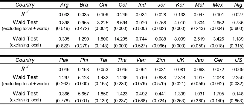
Following Harvey (1994), Table 2 present the results of estimating equation (5) by OLS for
each of the countries using the entire sample. The table depicts the R2 and two Wald tests
that help to understand whether local or both world and local variables are statistically
significant to explain the expected return of each country. That is, as long as equity markets
are affected for local (country) specific factors, correlations among country indices will be
low, then international portfolio diversification will, a priori, improve portfolio performance.
As can be seen from the table, for ten countries the linear model (equation (5)) exhibits
significance predictability. Notably, for all the developed countries, the model is significant.
On the other hand, for only five countries (Colombia, Korea, Malaysia, Mexico and
Philip-pines —all emerging economies-) local variables are statistically important to explain the
expected return.
Country Arg Bra Chi Col Ind Jor Kor Mal Mex Nig
R2 0.033 0.035 0.109 0.249 0.034 0.028 0.133 0.047 0.101 0.027
Wald Test 0.898 0.955 3.225 8.694 0.920 0.768 4.010 1.304 2.962 0.736
(excluding local + world) (0.519) (0.472) (0.002) (0.000) (0.500) (0.632) (0.000) (0.243) (0.004) (0.660)
Wald Test 0.305 1.290 1.800 14.295 0.744 0.088 8.039 2.519 3.426 1.189
(exclusing local) (0.822) (0.279) (0.148) (0.000) (0.527) (0.966) (0.000) (0.059) (0.018) (0.315)
Country Pak Phi Tai Tha Ven Zim UK Jap Ger US
R2 0.046 0.163 0.053 0.045 0.064 0.031 0.081 0.068 0.072 0.069
Wald Test 1.267 5.123 1.482 1.236 1.799 0.838 2.314 1.917 2.048 2.250
(excluding local + world) (0.262) (0.000) (0.165) (0.280) (0.079) (0.570) (0.021) (0.059) (0.042) (0.032)
Wald Test 0.366 5.657 1.850 1.423 0.492 0.441 1.339 1.031 1.795 0.148
[image:14.612.103.511.495.670.2](exclusing local) (0.778) (0.001) (0.139) (0.237) (0.688) (0.724) (0.263) (0.380) (0.149) (0.863) p-values are reported between brackets
Table 2
Mean equation estimations
OLS regression of the excess return of each country onto local and global information set of the investor. The global variables are a constant, the lagged world return, the lagged default spread (defined as the yield difference between Moody's BAA and AAA rate bonds), the month to mouth change in the U.S. term premium (measure by the yield on the ten-year U.S. Treasury note in excess of the one-month T-Bill rate), the lagged MSCI world dividend yield and the lagged Eurodollar rate. On the other hand, local ones includes the lagged local return, lagged dividend country dividend yield and the change in the exchange rate between the local currency and the US dollar.
Regarding the percentage of the sample variability explained by the model, for five
tries (Chile, Colombia, Korea, Mexico and Philippines), the R2 is higher than 10%. Note
that these five countries are emerging economies. For the rest of the sample the coefficient
of determination range from 3% to 8%.
It is important to mention, that even though Harvey (1994) used a different sample period
(and more countries), my results are similar. As in his paper, the main message of these
estimations is that emerging equity markets seems to be more predictable than developed
ones; consequently, exploiting these characteristics in the portfolio diversification problem
may lead to significant improvement in portfolio performance.
Finally, it is important to note, that the analysis of this section was performed using the
entire sample. In contrast, when estimating the “ex ante” expected gain of international
diversification, I run out-of-sample regressions to predict the expected return and omit the
"looking ahead bias" in my estimations. Unfortunately, this implies that for the former
out-of-sample estimations I am using less information than for the later ones.
4.2
Conditional Variance-Covariance Matrix
Given the methodology described in the previous section the only parameters that I need
to estimate are the elements of the matrices C, A and B, since the conditional
variance-covariance matrix has the following form: Ht = C +A ∗(εt−1εt−1) +B ∗ Ht−1,(where * denotes the Hadamard product of two matrices). The estimation of these parameters and
their respectively bootstrapped standard errors using the whole sample, are reported in Table
3.
Most of the coefficients of A and B are significant, at the standard levels. Moreover,
all diagonal coefficients in these two matrixes are highly significant with the exception of
Korea and Nigeria for matrix A and Venezuela for matrix B. At the same time, some well
known, nevertheless interesting, results arise from this table. The estimations suggest that,
consistent with the GARCH literature, aii+bii are close to one for most of the cases. That
is, the conditional variance for the index return for each country is a very persistent process.
15
Matrix A
Arg Bra Chi Col Ind Jor Kor Mal Mex Nig Pak Phi Tai Tha Ven Zim UK Jap Ger US
Arg 0.3007 (0.0422)
Bra 0.1014 0.1264 (0.0345) (0.0636)
Chi 0.0622 0.0487 0.0445 (0.0101)
(0.0245) (0.0191) Col 0.0168 0.0329 0.0409 0.1209
(0.0085)
(0.0166) (0.0206) (0.0608) Ind 0.0028 0.0477 0.0549 0.0994 0.1445
(0.0014)
(0.0240) (0.0276) (0.0500) (0.0727) Jor 0.0135 0.0049 0.0262 -0.0048 0.0331 0.1209
(0.0068)
(0.0524) (0.0068) (0.0024) (0.0038) (0.0260)
Kor 0.0390 0.0229 0.0342 -0.0049 0.0479 0.0047 0.1624 (0.0196)
(0.0115) (0.0172) (0.0025) (0.0241) (0.0001) (0.1817)
Mal 0.0511 0.0116 0.0840 0.0057 0.0089 0.0237 0.0524 0.1851 (0.0257)
(0.0058) (0.0221) (0.0028) (0.0045) (0.0119) (0.0264) (0.0025)
Mex 0.0401 0.0798 0.0542 0.0149 0.0743 0.0500 0.0224 0.0771 0.1557 (0.0011)
(0.0401) (0.0273) (0.0003) (0.0112) (0.0252) (0.0113) (0.0388) (0.0517)
Nig 0.0484 0.0116 0.0244 -0.0094 0.0211 0.0143 0.0118 0.0222 0.0614 0.1599 (0.1342)
(0.0058) (0.0123) (0.0047) (0.0061) (0.0072) (0.0060) (0.0112) (0.0309) (0.1004)
Pak -0.0068 0.0335 0.0531 0.0824 0.0817 0.0043 0.0082 0.0575 0.0617 0.0425 0.1532 (0.0034)
(0.0169) (0.0267) (0.0282) (0.0411) (0.0022) (0.0041) (0.0018) (0.0310) (0.0214) (0.0771)
Phi 0.0567 0.0204 0.0237 0.0142 -0.0033 0.0037 0.0208 0.0835 0.0233 0.0237 0.0049 0.0822 (0.0285)
(0.1102) (0.0119) (0.0071) (0.0017) (0.0019) (0.0105) (0.0420) (0.0117) (0.0119) (0.0025) (0.0414)
Tai 0.0105 0.0239 0.0344 0.0108 0.0305 0.0089 0.0514 0.0469 0.0448 0.1026 0.0707 0.0391 0.1129 (0.0053)
(0.0120) (0.0173) (0.0054) (0.0085) (0.0045) (0.0258) (0.0236) (0.0225) (0.0516) (0.0356) (0.0197) (0.0568)
Tha 0.0937 0.0528 0.0521 0.0068 0.0342 0.0024 0.0993 0.1012 0.0731 0.0990 0.0414 0.0797 0.1061 0.1592 (0.0374)
(0.0266) (0.0249) (0.0034) (0.0172) (0.0012) (0.0500) (0.0509) (0.0368) (0.0498) (0.0208) (0.0401) (0.0534) (0.0471)
Ven 0.1016 0.0253 0.0377 -0.0047 0.0269 0.0687 0.0100 0.0745 0.0856 0.0626 0.0085 0.0341 0.0189 0.0577 0.1090 (0.0374)
(0.0127) (0.0115) (0.0024) (0.0136) (0.0346) (0.0050) (0.0375) (0.0511) (0.0365) (0.0043) (0.0172) (0.0095) (0.0101) (0.0548)
Zim 0.0546 0.0260 0.0580 0.1059 0.0858 0.0015 0.0104 0.0608 0.0385 0.0045 0.1150 0.0304 0.0359 0.0414 0.0170 0.1863 (0.0275)
(0.0131) (0.0292) (0.0534) (0.0432) (0.0007) (0.0052) (0.0306) (0.0194) (0.0023) (0.0364) (0.0153) (0.0180) (0.0208) (0.0086) (0.0212)
UK 0.0608 0.0522 0.0364 0.0297 0.0530 0.0125 0.0567 0.0444 0.0513 0.0110 0.0190 0.0243 0.0169 0.0551 0.0360 0.0188 0.0520 (0.0020)
(0.0263) (0.0183) (0.0149) (0.0267) (0.0063) (0.0285) (0.0223) (0.0208) (0.0026) (0.0096) (0.0122) (0.0085) (0.0169) (0.0140) (0.0095) (0.0219)
Jap 0.0608 0.0125 0.0262 0.0356 0.0612 0.0079 0.0406 0.0152 0.0439 0.0212 -0.0011 0.0205 -0.0001 0.0417 0.0458 0.0424 0.0344 0.0846 (0.0306)
(0.0063) (0.0132) (0.0179) (0.0308) (0.0040) (0.0103) (0.0076) (0.0221) (0.0106) (0.0006) (0.0103) (0.0001) (0.0069) (0.0231) (0.0213) (0.0088) (0.0422)
Ger 0.0034 0.0574 0.0399 0.0141 0.0571 0.0139 0.0795 0.0385 0.0650 0.0348 0.0662 0.0041 0.0646 0.0687 0.0096 0.0143 0.0421 0.0011 0.0914 (0.0017)
(0.0281) (0.0201) (0.0071) (0.0287) (0.0070) (0.0400) (0.0194) (0.0327) (0.0175) (0.0333) (0.0020) (0.0325) (0.0325) (0.0048) (0.0072) (0.0110) (0.0005) (0.0143)
US 0.0431 0.0538 0.0540 0.0225 0.0710 0.0552 0.0813 0.0890 0.0932 0.0270 0.0446 0.0404 0.0484 0.0863 0.0615 0.0404 0.0590 0.0374 0.0689 0.1019 (0.0217)
[image:16.612.74.719.124.523.2](0.0271) (0.0272) (0.0233) (0.0657) (0.0124) (0.0411) (0.0448) (0.0469) (0.0136) (0.0225) (0.0203) (0.0112) (0.0299) (0.0310) (0.0204) (0.0297) (0.0153) (0.0003) (0.0389) Bootstrap standard error are between brackets
Table 3
16
Matrix B
Arg Bra Chi Col Ind Jor Kor Mal Mex Nig Pak Phi Tai Tha Ven Zim UK Jap Ger US
Arg 0.6993 (0.0424)
Bra 0.7399 0.8603 (0.1441) (0.0895) Chi 0.6209 0.7188 0.7887
(0.2822)
(0.3267) (0.3585)
Col 0.5412 0.5980 0.5328 0.6790 (0.1446)
(0.2278) (0.2422) (0.1785) Ind 0.3960 0.3477 0.2258 0.3169 0.3520
(0.2118)
(0.0614) (0.1026) (0.0211) (0.1007) Jor 0.6667 0.7517 0.5039 0.5660 0.3854 0.7871
(0.3030)
(0.2504) (0.2290) (0.2479) (0.1575) (0.3577) Kor 0.4998 0.6716 0.5746 0.4971 0.1571 0.6110 0.7303
(0.0498)
(0.0733) (0.2612) (0.0936) (0.0032) (0.2140) (0.0003) Mal 0.6970 0.8000 0.7028 0.5940 0.3271 0.7027 0.6518 0.7661
(0.1317)
(0.0633) (0.3195) (0.0042) (0.0345) (0.3194) (0.1233) (0.0675) Mex 0.5504 0.6790 0.5532 0.5386 0.2327 0.6408 0.6363 0.6554 0.6366
(0.2130)
(0.1047) (0.4515) (0.1132) (0.1140) (0.2913) (0.1598) (0.2066) (0.2719) Nig 0.5753 0.7411 0.6408 0.5702 0.1820 0.5890 0.5942 0.6671 0.5967 0.8402
(0.1653)
(0.1428) (0.2912) (0.2113) (0.5551) (0.2570) (0.0992) (0.0392) (0.1465) (0.1349) Pak 0.6251 0.7094 0.4503 0.4336 0.3852 0.7174 0.5645 0.6316 0.5166 0.5196 0.8468
(0.1913)
(0.1070) (0.2047) (0.1971) (0.4350) (0.2984) (0.2194) (0.1953) (0.1348) (0.2362) (0.0941) Phi 0.6239 0.6812 0.5803 0.3835 0.3286 0.6068 0.5209 0.6483 0.5153 0.4365 0.6147 0.6683
(0.1472)
(0.0626) (0.2848) (0.1743) (0.0397) (0.1539) (0.1554) (0.1212) (0.0584) (0.1984) (0.3029) (0.3094) Tai 0.5259 0.6093 0.5917 0.4570 0.2077 0.5462 0.5830 0.6263 0.5731 0.4385 0.4033 0.5541 0.6464
(0.0043)
(0.0052) (0.9689) (0.0723) (0.0805) (0.1471) (0.0631) (0.2747) (0.1532) (0.0666) (0.1833) (0.1501) (0.0688) Tha 0.6670 0.7078 0.6166 0.5192 0.3849 0.6661 0.5771 0.6975 0.5630 0.4529 0.6538 0.6715 0.6037 0.7484
(0.0674)
(0.0134) (0.2690) (0.2011) (0.1172) (0.2483) (0.0137) (0.1430) (0.1701) (0.1943) (0.0041) (0.0060) (0.0984) (0.1761) Ven 0.1819 0.1764 0.1875 0.1647 0.1234 0.1358 0.1026 0.1737 0.1158 0.1268 0.1367 0.1544 0.1253 0.1805 0.0712
(0.0827)
(0.0802) (0.0852) (0.0749) (0.1561) (0.0617) (0.0466) (0.2789) (0.0526) (0.0569) (0.0621) (0.0702) (0.0557) (0.0821) (0.0824) Zim 0.7131 0.7429 0.6774 0.4667 0.3729 0.5900 0.4185 0.6830 0.4772 0.6033 0.5889 0.6329 0.4767 0.6320 0.1930 0.8137
(0.0806)
(0.1120) (0.3079) (0.0778) (0.0117) (0.2682) (0.0263) (0.3104) (0.2169) (0.1336) (0.1821) (1.2158) (0.0371) (0.0700) (0.0877) (0.0122) UK 0.7335 0.8802 0.7355 0.5759 0.3025 0.7719 0.7418 0.8216 0.7110 0.7617 0.7416 0.7045 0.6496 0.7284 0.1585 0.7301 0.9308
(0.0024)
(0.0213) (0.3343) (0.1485) (0.0285) (0.3793) (0.0376) (0.0888) (0.2288) (0.1609) (0.1242) (0.1723) (0.0519) (0.0674) (0.0714) (0.0053) (0.0157) Jap 0.6232 0.7747 0.6705 0.4430 0.2027 0.6461 0.6733 0.7189 0.6177 0.6849 0.6397 0.6284 0.5803 0.6232 0.1232 0.6454 0.8407 0.7886
(0.0220)
(0.1064) (0.3048) (0.0101) (0.0098) (0.2937) (0.0579) (0.1224) (0.2108) (0.0174) (0.0195) (0.0006) (0.1515) (0.0559) (0.0560) (0.1148) (0.0966) (0.1485) Ger 0.7064 0.8301 0.7466 0.5086 0.2844 0.7097 0.7085 0.7971 0.6799 0.6436 0.6544 0.7345 0.7041 0.7453 0.1611 0.7095 0.8809 0.8051 0.8980
(0.0453)
(0.2523) (0.3393) (0.0937) (0.0888) (0.3226) (0.0839) (0.5565) (0.2539) (0.0212) (0.1066) (0.0392) (0.1738) (0.1287) (0.0478) (0.0665) (0.1044) (0.1322) (0.0974) US 0.7119 0.8497 0.7725 0.5799 0.2837 0.7106 0.7306 0.8083 0.6857 0.7283 0.6833 0.6909 0.6608 0.7289 0.1717 0.7157 0.8971 0.8131 0.8686 0.8898
(0.1014)
(0.0343) (0.3511) (0.1123) (0.0681) (0.2919) (0.0050) (0.1856) (0.1806) (0.1749) (0.1633) (0.0939) (0.1194) (0.0001) (0.0780) (0.0281) (0.0135) (0.0744) (0.0903) (0.0269) Bootstrap standard error are between brackets
Table 3 (continued)
[image:17.612.68.730.131.534.2]17
Matrix C
Arg Bra Chi Col Ind Jor Kor Mal Mex Nig Pak Phi Tai Tha Ven Zim UK Jap Ger US
Arg 0.3263 (0.3181)
Bra 0.1670 0.0829 (0.3207) (0.2390)
Chi 0.1666 0.1229 0.1286 (0.2889)
(0.3158) (0.3519)
Col 0.0875 0.0871 0.0636 0.1565 (0.0405)
(0.0266) (0.0631) (0.0658)
Ind 0.2493 0.2287 0.1608 0.0309 0.5712 (0.2464)
(0.3484) (0.0420) (0.0042) (0.2798)
Jor 0.0132 0.0057 0.0188 0.0211 0.0372 0.0254 (0.0784)
(0.0018) (0.0031) (0.0013) (0.0166) (0.1529)
Kor 0.1206 0.1204 0.1026 0.0393 0.1308 0.0045 0.1880 (0.1424)
(0.2021) (0.1341) (0.0044) (0.0157) (0.0140) (0.1816)
Mal 0.0891 0.0584 0.0571 0.0263 0.0934 0.0123 0.0607 0.0755 (0.1341)
(0.1115) (0.0884) (0.0006) (0.0553) (0.0165) (0.0537) (0.1261)
Mex 0.4004 0.1798 0.1739 0.0659 0.1648 0.0121 0.1257 0.1215 0.3466 (0.4091)
(0.3735) (0.1200) (0.0069) (0.0177) (0.0123) (0.1197) (0.1970) (0.3082)
Nig 0.0850 0.0512 0.0144 0.0513 0.0507 -0.0007 0.0202 0.0038 0.0352 0.0670 (0.0330)
(0.0491) (0.0363) (0.0173) (0.0485) (0.0270) (0.0279) (0.0279) (0.0114) (0.0245)
Pak 0.0629 0.0356 0.0273 0.0548 0.0911 0.0089 0.0454 0.0217 0.0720 0.0174 0.0189 (0.0224)
(0.0588) (0.0235) (0.0331) (0.0437) (0.0234) (0.0356) (0.0820) (0.1327) (0.0123) (0.0433)
Phi 0.1062 0.1252 0.1279 0.0590 0.0537 0.0079 0.1449 0.1420 0.1488 -0.0162 0.0140 0.3557 (0.0781)
(0.0962) (0.0421) (0.0295) (0.0023) (0.0113) (0.0150) (0.0715) (0.0225) (0.0140) (0.0103) (0.2207)
Tai 0.3555 0.2169 0.1587 0.1444 0.1353 0.0063 0.1334 0.1650 0.2320 0.0521 0.0496 0.2237 0.5480 (0.2595)
(0.3001) (0.1825) (0.0599) (0.1128) (0.0007) (0.1221) (0.2212) (0.1444) (0.0034) (0.0852) (0.0511) (0.2745)
Tha 0.0977 0.0834 0.0847 0.0455 0.1095 0.0305 0.0926 0.1059 0.1704 0.0196 0.0428 0.1624 0.1569 0.1808 (0.1566)
(0.1103) (0.1161) (0.0005) (0.1068) (0.0065) (0.1477) (0.1726) (0.0947) (0.0788) (0.0771) (0.0961) (0.1508) (0.4227)
Ven 0.3366 0.1939 0.0560 0.1393 0.1817 0.0256 0.0213 0.0431 0.1738 0.0908 0.0345 0.1098 0.0669 0.0115 2.0106 (0.5406)
(0.0256) (0.0924) (0.0327) (0.0163) (0.0688) (0.0167) (0.0062) (0.2193) (0.0119) (0.0987) (0.0002) (0.1237) (0.0851) (0.9197)
Zim 0.0145 0.0351 0.0214 0.0834 0.0652 0.0094 0.0250 0.0401 0.0237 0.0396 0.0185 0.0400 0.0487 0.0373 0.1540 0.0598 (0.0218)
(0.0138) (0.0582) (0.0022) (0.0254) (0.0240) (0.0260) (0.0561) (0.0573) (0.0125) (0.0219) (0.0025) (0.0059) (0.0117) (0.1743) (0.0320)
UK 0.0480 0.0212 0.0291 0.0260 0.0419 0.0086 0.0316 0.0200 0.0524 0.0078 0.0086 0.0473 0.0590 0.0292 0.0775 0.0061 0.0056 (0.0337)
(0.0403) (0.0327) (0.0098) (0.0125) (0.0173) (0.0173) (0.0257) (0.0299) (0.0060) (0.0043) (0.0160) (0.0194) (0.0285) (0.0332) (0.0057) (0.0017)
Jap 0.0456 0.0584 0.0273 0.0039 -0.0107 -0.0029 0.0866 0.0432 0.0648 0.0342 -0.0061 0.0833 0.0901 0.0395 0.0400 0.0179 0.0212 0.0867 (0.1248)
(0.1687) (0.1037) (0.0061) (0.0271) (0.0145) (0.1255) (0.0722) (0.1217) (0.0132) (0.0167) (0.0088) (0.0366) (0.0691) (0.0042) (0.0278) (0.0243) (0.1690)
Ger 0.0622 0.0336 0.0300 0.0288 0.0593 0.0119 0.0176 0.0336 0.0685 0.0224 0.0132 0.0603 0.0654 0.0507 -0.0397 0.0101 0.0102 0.0257 0.0134 (0.0635)
(0.0603) (0.0811) (0.0009) (0.0166) (0.0349) (0.0189) (0.0247) (0.0998) (0.0032) (0.0131) (0.0010) (0.0284) (0.0425) (0.0165) (0.0033) (0.0023) (0.0118) (0.0736)
US 0.0462 0.0214 0.0256 0.0265 0.0249 0.0044 0.0228 0.0146 0.0500 0.0083 0.0043 0.0393 0.0453 0.0235 0.0252 0.0047 0.0056 0.0161 0.0081 0.0053 (0.0652)
(0.0037) (0.0489) (0.0185) (0.0014) (0.0180) (0.0339) (0.0181) (0.1116) (0.0149) (0.0298) (0.0233) (0.0913) (0.0155) (0.1787) (0.0072) (0.0082) (0.0465) (0.0278) (0.0191)
Bootstrap standard error are between brackets
Table 3 (continued)
[image:18.612.60.725.99.499.2]economies the results are similar (Brazil 0.98, Philippians 0.92). Nonetheless, in some
cases like India, the conditional variance is not as persistent as (aii+bii= 0.49).
With this estimation in hand, get the conditional covariance matrix is trivial: Hˆt =
ˆ
C+ ˆA∗(et−1et−1) + ˆB∗Hˆt−1. As in the previous section, these estimations were performed using the complete sample. When estimating the “ex-ante” economic gain of including
emerging equity market holding in an international diversified portfolio, rather than used
this estimates, I perform out-of-sample estimation of the conditional covariance matrix. The
same caveats for the estimation of the expected return apply here.
4.2.1 Specification Test
The econometric theory behind the estimation procedure suggested by Ledoit et al (2003)
and the one used in this paper relays in the assumption that the standardized residuals
t = Ht−1/2εt, where Ht in the true conditional covariance matrix at time t, should have
constant covariance matrix equal to the identity matrix and the cross-product t 0t should be
uncorrelated over time. For this reason, if the empirical model used in this paper to analyze
the economics value of diversifying into emerging markets is correctly specified, I should
expect that the standardized residualsˆ = ˆHt−1/2et, are uncorrelated over time, whereHˆt is
the estimated conditional covariance matrix.
The natural way to test this hypothesis is to use the Ljung-Box test. While this test
is suitable for univariate analysis, the Ljung-Box statistic has the following problem for
performing the specification test required in this paper, as Ledoit et al (2003) highlight.
First, this test is designed to analyze univariate series, not matrix time series. Even more
important, under the null hypothesis, the asymptotic distribution is χ2
k, only if the data is
i.i.d.. Especially if the data is dependent theχ2
kapproximation may imply misleading results
(Romano and Thombs (1996)). To overcome this problem I use the statistic proposed by
Ledoit et al that only requires, under the null hypothesis, that the cross-products of the
LBcomb(k) =
X
1≤i≤j≤N
LBij(k) (7)
where LBij(k) is the univariate Ljung-Box for the series {ˆi,tˆj,t}. As they propose, the
p-value for this statistic is computed by the following sub-sampling method. Let denote
LBcomb,t,b(k) be the statistic based on the following data: {ˆt, ...,ˆt+b−1} for t = 1, . . . , T − b−1. So, calculating all the possibleLBcomb,t,b(k) for the sample, the sub-sample p-value is
given by4:
P VSub =
#{LBcomb,t,b(k)≥LBcomb(k)}
T −b+ 1 (8)
For this paper, the statistic and the p-value fork = 12and b= 50is: LBcomb(k) = 364.79
with p-value= 0.2201. That is, we do not reject the null hypothesis of no autocorrelation
(similar results were found using different k and b).
In short, this implies that the time series parsimonious model used to capture the dynamic
of the conditional variance-covariance model is correctly specified.
4.2.2 Conditional out-of-sample covariance
This subsection analyses the dynamic of the conditional correlation based on the estimation
of the Flexible Multivariate GARCH model. Special attention is placed on the conditional
covariance between the US and the rest of the countries in the sample.
Before commenting on the main characteristics of these conditional correlatione, let me
explain the observation used for the out-of-sample analysis. The out-of-sample exercise
begins on January 1990, so the first econometric estimation used only 59 observations. Of
course, when performing the subsequent estimations, the information that was used increased
with the periods.
4For details about sub-sampling test please see Ledoit et al (2003) and Politis, Romano and Wolf (1999,
chapter 3).
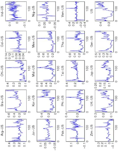
Figure 1 provides the conditional out-of-sample correlation between US returns and the
nineteen countries returns in the sample and the conditional US equity variance. Thisfigure
illustrates that the conditional covariance between two countries (in this case US with the
remain of the sample) are clearly time varying. In this sense, using unconditional analysis as
some of the existing literature has used (Li et al (2003) and Li (2003)) would lead to incorrect
results. Moreover, this time-varying correlation among securities justifies the choice of the
Flex Multivariate GARCH rather than alternatives multivariate GARCH model that impose
ad-hoc restrictions in the correlation coefficients (as in Bollerslev (1990) or Ding and Engle
(1994) to mention only a few) .
The dynamics of the conditional out-of-sample correlation is very diverse. For example,
for the Germany-US case, the figure depicts an upward sloping. That is, while around
January 1990 the conditional covariance was approximate 0.10, at the end of the sample
period, it was close to 0.40. On the other hand, there are some cases where the conditional
correlation is close to zero during the entier sample period. For Venezuela, ignoring the
two peaks, the plot shows that the equity index of this country was basically conditonal
uncorrelated with the US index.
In any case, the schemes clearly show that the correlations are time-varying and therefore
considering these movements in the optimization problem would be essential.
4.3
E
ffi
cient frontier
As was explained in section 2.1, I consider three types or portfolio selection problems. First,
I allow the investor to choose only among developed countries equity indices and the risk
free bond. Then, I solve the same problem assuming that the investor not only is able to
invest in developed equity markets and a risk free bond, but also in emerging market indices.
Finally in order to be more realistic, the opportunity investment set is given by: the four
developed indices, risk free bond and the sixteen emerging market equities, but imposing a
20 % cap in the total holding of developing economies.
The efficient frontiers calculated at each point in time, using the out-of-sample
estima-tions, are reported in Figure 2.
As can be seen from the figures, the efficient frontier has dramatically moved over time.
So, performing unconditional analysis when estimating the economics or statistical benefit
Comparing panels A and B, it can be seen that the efficient frontiers move northeast when
emerging markets assets are included in the investment opportunity set. By inspection, we
can say that these movements are significant, since most of the portfolios depicted in the
efficient frontier for developed market case have expected annual return less than 20% while,
if the investor incorporates emerging equity markets, more than half of the portfolios have
annual expected return that exceed 40%. At the same time, the standard deviation for each
of the portfolios is generally lower in panel B, compared to panel A.
This evidence persists when a 20% cap is introduced in the problem (panel C). That is, the
efficient frontiers move northeast, relative to panel A, but the movement is less dramatic than
in panel B. Contrasting panels B and C, the estimation implies that the realistic upper bound
constraint in investing in developing equity markets shifts the efficient frontier considerably.
In short, the efficient frontier in panel C are, as expected, between those in panel A and B.
As I mention in section 2.1, the economic measure used in this paper is based on the
comparison of the efficient frontier between panel A and C. But contrary to previous
litera-ture, this paper goes one step further. Instead of comparing Sharpe Ratios or other measures
that are independent of the risk tolerance, I use a utility based certainty equivalent rate of
return; so, even though each investor (with different risk aversion coefficient) will choose
the same risky portfolio at each point in time (given the efficient frontier that he faces at
period t), thefinal weights between risky and risk free assets will depend on the preference.
Consequently, the out-of-sample maximum fee that an investor is wiling to pay to switch
from the ex-ante optimal portfolio when he is only able to invest in equities from developed
economies, to the ex-ante optimal portfolio including, also developing economies securities,
depends on the risk aversion coefficient. As it is show in this paper in subsequent sections,
including the risk tolerance in the analysis is not irrelevant.
The main message of the analysis of the dynamic of the efficient frontier is that given the
theoretical framework used in most of the literature that analyzes the benefit of diversifying
into emerging equity market and the one used in this paper; ignoring the time-varying
investment opportunity set, that is, ignoring the fact the mean-variance frontier varies over
time, would be crucial.
4.4
Economic gains
This section reports the main contribution of this paper. Here, I analyze not only the
economic value of diversifying into emerging equity markets using a utility-based measure,
but also I investigate its dynamics by studying the effect of the time-varying economic
environment in the proposed measure.
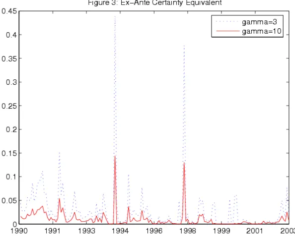
Figure 3 contain plots of the “ex-ante” certainty equivalent rate of return (at each point
in time) for a quadratic utility investor for two different relative risk aversion coefficients
(γ = 3,10). That is, this figure shows the λt that solves equation (4) for different risk
tolerance coefficients. As I mention earlier, the proper way to interpret this measure is as
the risk free annual rate that makes the investor indifferent between holding the optimal
diversified portfolio (that is, including both emerging and developed equity markets) versus
a portfolio of only developed equity markets.
The estimated series reveals interesting results. First, independent of the preference
(risk aversion), the diversification benefits change across time. That is, the utility-based
economic measure moves considerably as time evolves. Consequently unconditional analysis
utility function plays an important role in the estimation. Intuitively, it primarily affects
the level of the estimated certainty equivalent rate rather than its dynamics. Consistent
with Li (2003), the expected utility benefits of expanding the investment opportunity set
with emerging equity markets is bigger for the less risk averse investor. Along all
out-of-sample periods, the investor with relative risk aversion equal to 3 is at least as willing to
pay than the least risk tolerant one at each point in time. The intuition is because the more
conservative investor invests a larger fraction of his wealth in risk free asset, and therefore
faces less variation across models.
5% 3% 1% 0.5%
3 3.00% 5.08% 43.97% 0.00% 16.00% 30.63% 52.50% 67.50% 0.83%
10 1.00% 1.70% 14.45% 0.00% 2.00% 6.88% 28.75% 49.38% 0.22% Unconditional
[image:26.612.157.454.286.531.2]Case
Table 4
Summary Statistics: Ex-ante Certainty Equivalent (Jan 1990 - Apr 2003)
Percentage above Risk Aversion Coefficient Mean Std Dev Max Min
Table 4 summarizes the above estimations. On average, the riskiest investor is willing to
pay up to 300 basis points annually, in order to increase his investment opportunities. At
the same time, the economic measure for this investor ranges from 0% to 43%. The results
are less volatile for the less risk-tolerant agent. His certainty equivalent rate goes from 0%
to 14%, with standard deviation of 1.7%. Even for this investor, on average, 100 basis points
annually is the ex-ante maximum fee that he is willing to pay to diversify into emerging
equity markets. Furthermore, ignoring the two spikes the average certainty equivalent rate
are 2.53% and 0.81 % for γ = 3 and γ =10, respectively. Note that as Table 4 reveals, in
more of the 16 percentage of the out-of-sample months the γ = 3 investor was willing to
pay more than 5 % and more than half of the time 100 basis points, always on an annual
basis. On the other hand, half of the times the conservative agent was willing to pay up to
50 basis points. Finally, note that the certainty equivalent rate using unconditional mean
and covariance matrix (last column of Table 4) produces totally misleading results.
To sum up, from this first inspection of the economic gains, it is important to highlight
that the certainty equivalent rate varies across time and that the investor’s risk tolerance
affects this measure. Thus, any analysis of the value of including emerging equity market in
an international diversify portfolio should contemplate these two issues.
4.4.1 Statistical Significance of the Certainty Equivalent
Due to the subsequence non-linear transformation in the estimation procedure, given that
I need to preserve the predictability of the returns and using the fact that ultimately, all
the estimations performed in this paper depend on the errors of equation (5), the natural
way to have a description of the sampling properties of my estimations, is performing the
following bootstrapping exercise. First I randomly draw (with replacement) 219 observations
(as the original sample size) from the errors calculated in the mean equation for each country.
Second, using the proper expected returns (that is, those consistent with the draws of the
previous step) I calculate the time series of the out-of-sample certainty equivalent rate using
equation (4) as I did with the actual data. Third, I repeat this procedure 10,000 times.
Finally, the sample standard deviation from this bootstrap experiment, at each point in
time, is the standard deviation of the utility based economic measure use in this paper.
Figures 4 and 5 display the certainty equivalent rate for relative risk aversion coefficients
just explained.
It is worth mentioning that the certainty equivalent rate is bounded below by zero since,
when choosing the optimal investment decision, the agent cannot be worse offwith a better
investment opportunity set. Therefore, the negative value consequence of subtracting 2
standard deviations, should not be consider as evidence that the agent needs to be paid
for improving his opportunity set, on the contrary, should be taken as in those period the
economics gain measure may not be relevant, that is, as if the certainty equivalent rate was
zero for those months.
Even though in the previous section I found significant economic gains, figures 4 and 5
reveal that for some month of the analized sample, the maximum fee that the investor is
willing to pay to enhance his choice set, may be just consequence of simple sample error.
Nevertheless, the pictures show that for more than half of the periods the economic gain is
still greater than zero after subtraction 2 standard deviations.
To be more concrete, for 53 % of the months analyzed in this paper, even after subtracting
2 standard deviations, the certainty equivalent rate was greater than zero. At the same time,
the mean of the lower bound plotted infigure 4 and 5 are 0.99 % and 0.39 %, respectively.
On the other hand, the mean of the upper bound are 4.54 % and 1.56%; in words, this imply
that from January 1990 to April 2003, the conservative investor was willing to pay annually,
on average, between 39 and 156 basis point, while the riskier one, between 99 and 454 basis
points.
I would like to comment that the principal aim of these estimations is simple to get an
approximate measure of potential economics benefit of diversifying into emerging markets,
not to quantify these gains to many decimal places. In this sense, the results showed so
far would imply that investor may found economically valuable including emerging equity
markets in an international diversified portfolio, even after consider short sale constrains and
not allowing the investor to allocate more than 20% of his wealth in emerging markets.
4.4.2 Economic gain and economic environment
The time series estimations of the expected gains from better diversification, allows me to
particular, the effect of emerging market crises, the US recession and the market liberalization
[image:30.612.151.462.218.463.2]process are studied.
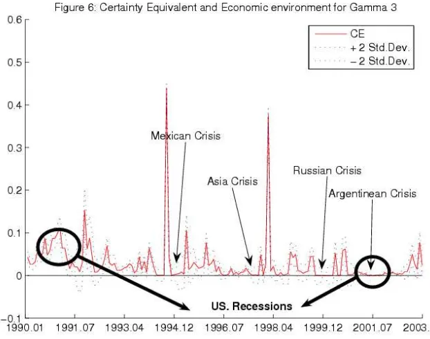
Figure 6 highlight the emerging market economic crises and the US recession periods (for
the horizon analyzed in this paper) in the estimated time series when investor’s relative risk
aversion coefficient is 35.
Let’s first focus on the emerging market crises. From the inspection of this picture, it
seems that whenever emerging countries had experienced an economic crises (Mexican Crisis
Dec-1994, Asian Crisis Jul-1997, Russian Crisis Nov-1999 and Argentinean Crisis Aug-2001),
the expected gain of including equity from this group of countries dropped virtually to zero.
The optimal weights for this quadratic utility investor in this group of countries almost
disappear. More precisely, while on average, he should invest 7% in emerging equity market
for the whole out-of-sample period, 0.81% is the “ex-ante” optimal weights during crises
times. That is, not only this mean-variance investor reduces, ex-ante, his position in the
country that is experiencing economic slow-down, but also he decides, basically, to disinvest
in all the emerging economies. It is important to note that for the Mexican crisis, the ex-ante
5The plot forγ=10 is qualitative identical, so it is omitted.
proportion of the wealth invested in emerging market dropped to 3% not virtually zero as
in the other cases. These results may be consequence of some of the implication, about
contagion, found in Bekaert et al (2004). Their analysis suggests that there was contagion
during the Asia crisis but it might not be during the Mexican one. In this sense, it might
be argue that the dynamic of the economic value estimated in this paper indicates that
the existence of contagion modifies the extent to which diversification of risk is possible for
investors (Goldstein and Pauzner (2004)).
Regarding to the US economics recession period, interesting results are illustrated in
Figure 6. During the out-of-sample horizon, the US economy had experience two recessions:
from July 1990 to March 1991 and from March 2001 to November 20016. Clearly, for thefirst
one, the "ex-ante" economics gain due to diversifying into emerging market was economically
different from zero. Actually, during this period, the average maximum annual fee that an
investor withγ = 3 was willing to pay to improve his investment set was 3.68 % (1.33 % for
γ = 10). For the March 2001- November 2001 recession, the results seems opposite to those
descried before, but as the reader may be thinking, it is not clear whether the irrelevance of
diversifying into emerging markets is due to US business cycle or emerging market crises. In
other words, it is difficult to perform a controlled analysis from the simple inspection of the
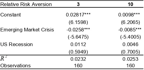
graph, therefore, in Table 5 I pretend to overcome this problem.
OLS regression with Newey-West consistent standard errors. The dependent variable is the certainty equivalent and the independent are dummy variables for emerging market crises and for US recessions.
Relative Risk Aversion 3 10
Constant 0.02817*** 0.0098***
(6.1598) (6.2065)
Emerging Market Crisis -0.0258*** -0.0085***
(-5.6475) (-5.4005)
US Recession 0.0112 0.0046
(0.5949) (0.7005)
R2 0.0232 0.0253
Observations 160 160
*,** and *** denotes significance at 10%, 5% and 1% respectively.
[image:31.612.182.420.561.678.2]Significance of emerging market crises and US recessions Table 5
This table presents the regression results of regressing the certainty equivalent rate onto
a constant, a dummy variables that takes one for any emerging market crises period and
a dummy variable equal to one when the US economy was in recession. The purpose of
this simple exercise is to have additional evidence about the potential effect of national
and international environment over the economic gain measure. The results are clear and
(qualitatively) do not depend on the risk tolerance coefficient. Crises in developing economies
statistically decrease, on average, the economic gain measure by 2.5% and 0.85% for γ = 3
and γ = 10 respectively; on the other hand, neither for the conservative, nor the riskier
investor seems to change the willingness to pay to enhance the opportunity set the US
economic recession. That is, this suggest that when US investors needed them the most, at
least during the sample period studied in this paper, emerging market economically improve
the investment opportunity set of these investors. At the same time, this result are not
sufficient to conclude that given the existence of the emerging markets crises, invest in
equity from these countries would not improve the portfolio performance. As long as crisis
in this part of the world are not predictable, investing in these equities is still optimal, since
on average the investor is getting, ex-ante, more utility.
Finally, following DeSantis and Gerard (1997), Figure 6 provides the low frequency
com-ponent of the estimated economic value (for both cases) to be able to study the effect of
market liberalization on the results discussed until now7. The reason of doing so is because
the liberalization process needs time to take place (Bekaert and Harvey (2000)), so
concen-trating in the trend component rather than on the row series might capture the main effect
of this phenomenon.
The filtered series despite in this figure suggest that the trend of the expected gain was
decreasing during the nineties. This might implicate that given that financial liberalization
should, a priory, increase the cross-country equity correlation, benefits of including emerging
markets into the opportunity set tend decrease as a consequence of this process. But from
2001 on, the expected gain measure shows an opposite trend (upward). Moreover, the nineties
was characterized for subsequence emerging market crises that, as it was shown, seems to
7The trend of the certainty equivalent was calculated using the commonly use HPfilter.
decrease the certainty equivalent rate. So I would like to argue that, time-clustered crises in
the developing countries are the main reason of this downward trend, rather the pour effect
of the market liberalization process. In any case, not only the low frequency component
presents an upward slope in end of the sample, but also, on average the economic magnitude
of the proposed measure is important (specially for the less risk averse investor), thus, the
empirical exercise developed in this paper suggest that economics value of diversifying into
emerging markets remains relevant even after the liberalization process.
5
Conclusions
In this paper I analyzed the “ex-ante” economics value of diversifying into emerging equity
markets from the US investor prospective, using a mean-variance framework. The novel
parts of my analysis are two. First, the value of diversifying into emerging equity markets
is estimated with an “ex-ante” utility based measure (which links the investor’s tolerance
to risk with her/his diversification decision) and using conditional information; and
and international economic environment affect the economic gain of better diversifying the
portfolio.
Interestingly, depending on risk tolerance characteristics, the value of diversifying into
emerging equity markets is estimated to be between 100 and 300 annual basis points, even
under a twenty percent cap in emerging market. Furthermore, the analysis indicates that
while emerging market crises seem to reduce these economic gains, when US economy is
in a recession, investing in emerging equity markets still helps to improve the portfolio
performance. At the same time, although in the early nineties a capital market liberalization
process took place, the gains of investing in emerging equities remain economically significant,
with a growing trend from 2001 on.
Although the main contribution of this paper is simple to get an approximate measure of
potential economics benefit of diversifying into emerging markets, not to quantify these gains
to many decimal places, the analysis omits important characteristics of emerging markets
equity returns. Ignore higher order moment in this analysis, like skewness and kurtosis,
when dealing with emerging market may be inappropriate, so introducing these dimensions
in the portfolio optimization problem would be interesting. More importantly, as most of
the literature related with this work, this paper, leaves the following fundamental question
unanswered: Which are the economics forces that are driving these results? this question
should be the focus of future research in this area of internationalfinance.
References
[1] Bekaert, G. and Urias, M.S. (1996). Diversification, Integration and Emerging Markets
Closed-End Funds. Journal of Finance. 51, 835-869.
[2] Bekaert, G., Harvey, C. R. and Ng A. (2004). Market Integration and Contagion. Journal
of Business, forthcoming.
[3] Bekaert, G. and Harvey, C. R. (2000). Foreign speculators and emerging equity market.
Journal of Finance. 55. 565-614.