“Essays on Trade and Technology”
Harald Fadinger
Universitat Pompeu Fabra
Department of Economics and Business
Director: Prof. Jaume Ventura
Author:
Harald Fadinger
11Address: Stenggstrasse 22, A-8043 Graz, Austria. E-mail: [email protected]; Phone: 635786917
i
Table of Contents ii
Acknowledgements iv
Introduction v
1 Productivity Differences in an Interdependent World 1
1.1 Introduction . . . 1
1.2 The Helpman-Krugman-Heckscher-Ohlin Model . . . 6
1.2.1 Assumptions and Setup . . . 6
1.2.2 Demand . . . 8
1.2.3 Behavior of Firms and Technology . . . 9
1.2.4 Equilibrium . . . 11
1.3 A Method for Productivity Calibration . . . 19
1.3.1 Using Trade Data to Evaluate the Model . . . 21
1.4 Results . . . 26
1.4.1 Development Accounting . . . 40
1.5 Conclusion . . . 43
2 Trade and Sectoral Productivity 45 2.1 Introduction . . . 45
2.2 Related Literature . . . 47
2.3 A Simple Model . . . 49
2.3.1 Demand . . . 50
2.3.2 Supply . . . 51
2.4 Towards Estimating Sectoral Productivities . . . 52
2.5 Results . . . 58
2.6 Robustness . . . 72
2.6.1 Hausman Taylor . . . 73
2.6.2 Heterogeneous Firms and Zeros in Bilateral Trade . . . 78
2.6.3 Eaton and Kortum’s (2002) Model . . . 81
2.6.4 Pricing to the Market and Endogenous Mark-ups . . . 83
2.6.5 Trade in Intermediates . . . 85
2.6.6 Comparing Estimates with Solow Residuals . . . 86
2.7 Productivity Differences and Theories of Development . . . 88
2.8 Conclusion . . . 95
Appendix Chapter 1 97 .1 Data . . . 97
.2 The Productivity Calibration Problem (PCP) . . . 99
.2.1 Uniqueness of Solution to PCP . . . 101
Appendix Chapter 2 103 .3 Data Description . . . 103
.4 Derivation of the Productivity Estimates with Heterogeneous Firms . 108 .5 Mismeasurement of Sectoral Factor Income Shares . . . 111
.6 A Two Country General Equilibrium Model . . . 113
.6.1 Romalis’ Model . . . 115
.6.2 A Ricardian Model . . . 116
The first big thanks goes to Jaume Ventura, whose fascinating lectures got me hooked
on the field of International Economics in the first place. Later on, when he became
my supervisor, his guidance was of course also of great value for the process of writing
this thesis. His critical comments and his sense for the essential helped me to master
some of the difficulties I faced, above all in the earlier phases of my research. I am
also indebted to Antonio Ciccone and especially to Gino Gancia for the numerous
discussions that substantially improved the quality of my research and their
encour-agement. I would also like to thank my coauthor Pablo Fleiss, who worked with me
on the second chapter of this thesis.
Moreover, I owe a thanks to my colleagues and friends Alessia Campolmi, Chiara
Forlati, Stefano Gnocchi, Antoni Rubi and Katharina Wick for many discussions,
support and their friendship. I am also indebted to the people at ECARES, Universite
Libre de Bruxelles, where I spent the last year of my doctoral studies and especially
to Paola Conconi. Not to be forgotten are of course the three Martas, who formed the
crew at the GPEFM office during most of my studies, and helped me to overcome all
the administrative hurdles I faced during my PhD - Marta Araguay, Marta Araque
and Gemma Burballa. Finally, I would like to acknowledge financial support from the
Austrian Academy of Science under a DOC-Scholarship during some of the period of
my doctoral studies at Universitat Pompeu Fabra.
Why are some countries so rich while others are so poor? Standard wisdom attributes
about half of the variation in cross country differences in income per worker to
differ-ences in productivity while the remaining half is seen to be due to differdiffer-ences in factor
endowments, such as human- and physical capital. The main topic of this thesis is
to combine insights from trade theory with those from the growth and development
literature to study cross country differences in productivity. In particular, I develop
tools that allow me to use the richness of information contained in trade data to
es-timate productivities both at the aggregate - factor specific - and at the sector level,
which enables me to obtain a number of new results on the reasons and the effects of
cross country variation in the efficiency of production.
In chapter one I build a quantitative world equilibrium model of trade, that
com-bines the Helpman and Krugman (1985) Heckscher-Ohlin cum intra-industry trade
model with factor specific cross country productivity differences. Since this model has
predictions both on income differences and the factor content of trade, I
simultane-ously fit data on income, factor prices and trade to estimate productivity differences
and the aggregate elasticity of substitution between human capital and physical
cap-ital. The results of my estimations show that human and physical capital are
com-plements at the aggregate level, thus rejecting a Cobb-Douglas production function.
I find that the productivity of human capital is much higher in rich countries than in
poor ones, while there is no clear relation between the productivity of physical capital
and income per worker.
In chapter two2 I design and apply a method to estimate cross country differences
in productivity at the sector level from bilateral trade data. I take and integrated
2This chapter is joint work with Pablo Fleiss.
Heckscher-Ohlin-Krugman-Ricardo approach, and estimate differences in sectoral
pro-ductivity as observed trade that cannot be explained by differences in factor
intensiti-ties and factor prices nor by differences in trade costs. The advantage of this endeavor
is that it helps to overcome data problems that render the application of standard
methods for computing sectoral productivities, which require comparable information
on inputs and outputs at the sector level, inadequate for most countries. I estimate
total factor productivity for 24 manufacturing sectors in more than 60 countries at
all stages of development. I find that productivity differences between rich and poor
countries are substantial and systematically more pronounced in sectors that are
in-tensive in human capital and research and development. Subsequently, I use these
estimates to test theories from the growth and development literature that have
im-plications for the the patterns of productivity differences across sectors, such as the
Productivity Differences in an
Interdependent World
1.1
Introduction
Finding answers to the question why some countries are so much richer than others
is one of the fundamental challenges in economics. While according to the consensus
view cross country differences in factor endowments and differences in productivity
are more or less equally important causes for the cross country variation in income
per worker (Caselli (2005)), there is little evidence whether individual economies
are actually well described by an aggregate Cobb-Douglas production function and
whether differences in productivity across countries are really factor neutral as usually
assumed in the quantitative growth literature.
Moreover, even though trade is empirically very important 1 and may also
poten-tially affect the shape of countries’ aggregate production possibility frontiers (Ventura
(2005)) most research in growth and development still uses closed economy models
when estimating cross country differences in productivity. This may not only be too
1In the early 1990ies trade already amounted to 38 per cent of world income and by the turn of the millennium it had reached 52 per cent of world output (Trade is measured as exports+imports, data are from the Penn World Tables 6.1.).
restrictive for theoretical reasons but - since these models have by their very nature
nothing to say about trade - it also leaves one of the best sources of cross country
information - bilateral trade data - completely unexploited.
A second, independent line of investigation in international trade deals with the
prediction of the Heckscher-Ohlin-Vanek (HOV) Theorem, that states that capital
abundant countries should export capital (through trade in goods), while labor
abun-dant countries should export labor. This research, which uses trade data to evaluate
the validity of this theory, finds that cross country differences in productivity greatly
help to explain factor flows embodied in trade.
The goal of this paper is to merge these two approaches by using a world
equi-librium model - the Helpman-Krugman-Heckscher-Ohlin (1985) model - to estimate
factor augmenting productivities, thereby providing a unified framework and
exploit-ing the information contained both in income and in trade data. This model has
been the workhorse of trade economists for more than two decades.2 It combines
inter-industry Heckscher-Ohlin trade with intra-industry trade due to increasing
re-turns and love for variety. I augment the model for differences in the efficiencies with
which factors are used across countries to introduce a potential role for productivity
in generating cross country variation in income per worker.
The model encompasses two very popular views of the world as particular cases.
The first one is the neoclassical one sector model with factor deepening that is the
standard framework in the quantitative growth literature, while the second one is
the Heckscher-Ohlin model with conditional factor price equalization, the canonical
model for estimating productivities in the trade literature (Trefler (1993), Trefler
(1995)). Cases of intermediate integration are described by a world that separates
into multiple cones of diversification, with different sets of countries specializing in
the production of different sets of goods.
I simultaneously fit data on income, endowments, factor prices and the factor
content of trade. This provides me with over-identifying restrictions that enable me
to calibrate productivities and at the same time allow me to evaluate the fit of the
model and to estimate the values of underlying parameters. More specifically, I test
the factor deepening case against cases with multiple cones of diversification and
ones where conditional factor price equalization occurs and I estimate the elasticity
of substitution between human and physical capital.
My main findings are that the factor deepening model with factor specific
pro-ductivities and weak complementarity between human and physical capital vastly
outperforms the other versions of the model considered in this paper. In particular,
the elasticity of substitution between human and physical capital is estimated to be
significantly lower than one, so that the Cobb-Douglas model is clearly rejected. Rich
countries have far higher productivities of human capital than poor ones, while there
is no clear relation between physical capital productivity and income per worker.
Moreover, my results imply that the model best supported by the HOV Theorem has
no Heckscher-Ohlin motiv for the exchange of goods and all trade is due to increasing
returns and love for variety.
In terms of intellectual ancestors, this paper integrates two lines of investigation.
The first one is the literature on development accounting, which uses income and
endowment data to measure productivity differences. Some of the classical
contri-butions are due to King and Levine (1994), Klenow and Rodriguez-Clare (1999),
Prescott (1998) and Hall and Jones (1999). See Caselli (2005) for a survey. A stable
result of these studies is that total factor productivity is strongly positively correlated
of this variable. Caselli (2005) adds factor specific technology differences to this
ap-proach and discovers that rich countries have higher productivities of human capital
than poor ones, whereas poor countries have higher productivities of physical capital
than rich nations.
The second strand of research, that uses trade data to measure productivity
differ-ences, is the literature that tests the prediction of the Heckscher-Ohlin-Vanek (HOV)
equations. They state that countries’ trade structure is such that they are net
ex-porters of the services of those factors, in which they are more abundant than the
world average. A seminal contribution by Trefler (1993) shows how the HOV
equa-tions can be used to solve for the unknown factor specific productivities of each
country that equalize measured and predicted factor flows under the assumption that
differences in factor prices across countries are caused exclusively by variation in
fac-tor productivities. He finds that rich countries have both higher productivities of
labor and physical capital than poor countries.
In another important paper Davis and Weinstein (2001) relax the assumption that
differences in factor prices are caused only by differences in productivities. They show
that both Hicks-neutral differences in total factor productivity, which they estimate
using input-output data, and local factor abundance must be taken into account in
order to improve the fit of the HOV equations. However, their sample is limited
to ten large OECD countries, so that they have nothing to say about productivity
differences between rich and poor countries.
This paper goes beyond the previous contributions because I allow both for factor
productivities and local factor abundance to matter for income differences and I
match data on income, factor prices and trade at the same time. Also, since I put
more structure on the underlying model, I am able to estimate the value of underlying
Turning to the evidence on the aggregate elasticity of substitution between capital
and labor, a long line of studies, summarized by Hamermesh (1986), have attempted
to estimate this parameter at various levels of aggregation and using both cross section
and time series data. Despite of this, the evidence on its value remains inconclusive,
which may potentially reflect mis-specification because this body of research
consid-ers exclusively Hicks neutral technological change. Recently, Antras (2004) discusses
the bias that arises from this restriction and estimates the elasticity of substitution
between capital and labor for the US economy allowing for factor augmenting
produc-tivity differences using time series data. In line with my results, most of his estimates
are significantly lower than one.
Finally, Waugh (2007) performs a development accounting exercise in an open
economy framework that extends Eaton and Kortum (2002). However, he restricts his
analysis to Cobb-Douglas production technology and his main interest is to investigate
the role of trade in accounting for cross country income differences.
Summing up, the main contributions of this paper are threefold: Firstly, it
inte-grates development accounting with trade theory and methods. Secondly, the paper
proposes to introduce formal over-identification using data from outside the model to
evaluate the fit of the productivity calibrations. Thirdly, this buys me a very precise
estimate of the elasticity of substitution between human and physical capital, a clear
rejection of the aggregate production function being Cobb-Douglas and the possibility
to test which model performs best in terms of fitting the HOV equations.
The outline of the paper is as follows: In the next section I develop a theoretical
model of the world economy with trade due to factor proportions and love for
va-riety that includes factor specific cross country productivity differentials. In section
three I show how factor productivities can be recovered from the model when data
equations can be used in this framework to evaluate the plausibility of the calibrated
productivities and to estimate the values of underlying parameters. In section four I
present the results of calibrating productivities in the
Helpman-Krugman-Heckscher-Ohlin framework and use the calibrated productivities to perform a development
accounting exercise. The last section concludes.
1.2
The Helpman-Krugman-Heckscher-Ohlin Model
1.2.1
Assumptions and Setup
The model presented in this section is a standard model of international trade. There
are two reasons for trade in this environment. The first one is due to increasing
returns. Consumers value variety and each variety is produced by a monopolist
because increasing returns are internal to the firm and new varieties can be invented
without cost. Since consumers want to consume all varieties each producer serves
the world market for her particular variety, which leads to trade within sectors. The
second motive for trade is factor proportions. There exist many sectors each of
which uses factor inputs with distinct intensities and countries differ in the ratios of
their endowments. This gives rise to Heckscher-Ohlin trade and countries produce
on average more varieties in those sectors that use its relatively abundant factor
intensively. I also introduce cross country differences in the productivities with which
factors are used in production, so that a given amount of human or physical capital
leads to a different amount of production, depending on the country where production
is performed.
The Heckscher-Ohlin part of the model adds two main effects to the standard
model used in the development accounting literature. The first one is structural
factor endowments. Countries which are abundant in physical capital will concentrate
their production in sectors that are intensive in this factor. This tends to increase the
role of variation in factor endowments in explaining cross country income differences
because countries can employ their factors more efficiently. The other one is terms
of trade. These work exactly in the opposite direction because they depress the
income of those countries that produce goods which are intensive in the globally
abundant factor, thereby reducing the importance of factor endowments in accounting
for income differentials. The monopolistic competition part is introduced mainly to
explain trade in the absence of differences in factor proportions, as is the case in
the standard model for development accounting, but it has no important impact on
countries’ aggregate production possibility frontiers.
The flexible benchmark model of the world economy relies on the following main
assumptions.
A.1: Countries are open to trade in goods and possess perfectly competitive factor
markets.
A.2: Goods markets are monopolistically competitive.
A.3: Factors are immobile between countries and perfectly mobile within countries.3
A.4: Each country is endowed with human capital Hc and physical capital Kc.4
A.5: Productivity is specific to a factor located in a country.
3The immobility of labor is probably not a very controversial assumption. Even though some mobility of people can be observed, there exist very large barriers to migration from poor to rich countries. Starting at least with Lucas (1990) a large literature in International Economics has been dealing with the question why capital does not flow from rich to poor countries. Caselli and Feyrer (2006) make the interesting point that capital may actually be distributed quite efficiently across countries, so that there is no reason to observe large capital flows from rich to poor nations.
A.6: Each country has access to technologies to produce in I sectors, that vary in their capital intensities.
A.7: Consumers in all countries have identical, homothetic preferences with fixed
expenditure shares. 5
The model is then easily described by Assumptions A.1-A.7 and the specification
of demand and supply.
1.2.2
Demand
Consider a world economy with countries indexed by c ∈ C and sectors indexed by
i ∈ I.6 Assuming that trade is balanced, aggregate expenditure of country c equals
its aggregate income.
Ec=PcYc = I
X
i=1
Eic = I
X
i=1
βiEc, (1.1)
wherePcYcis GDP of country c in dollars, andYcis GDP in purchasing power parities
and is measured in aggregate consumption units. Aggregate spending is split across
I sectors with fixed expenditure shares βi.7
The ideal aggregate price index is Cobb-Douglas. It measures the minimum
ex-penditure to buy one unit of the aggregate bundle of goods.
Pc = I
Y
i=1
Pi
βi
βi
, (1.2)
where Pi are the sectoral price indices.
5This together withA.1implies that the optimal price index of Gross Domestic Product has the same form in all countries.
6I slightly abuse notation by denoting with C and I both the sets of countries and goods and their cardinalities.
Sectoral price indices are constant elasticity of substitution composites of the
prices of sector specific varieties.
Pi =
Z Ni
0
pi(n)1−σdn
1 1−σ
, (1.3)
where σ > 1 is the elasticity of substitution between any two varieties and Ni =
PC
c=1Nic is the total number of varieties produced in sector i.
The form of the sectoral price indices implies that there is love for variety and
aggregate consumption is increasing in the number of varieties available in each sector.
The demand function of country cfor variety n produced in countryc0 in sector i
implied by the price indices can be found from the sectoral price index by using Roy’s
law.
xicc0(n) =
pi(n)−σ
Pi1−σ βiEc (1.4)
1.2.3
Behavior of Firms and Technology
Final goods are freely traded and are produced by monopolistically competitive firms.
In each sector firms choose a variety and an optimal pricing decision taking as given
the decisions of the other firms in the industry.8 The output of an industry consists of
a number of varieties that are imperfect substitutes for each other. Production of each
variety is monopolistic because of economies of scale. In the model the invention of
a new variety is costless, so firms always prefer to invent a new differentiated variety
instead of entering in price competition with an existing firm.
In each country firms are homogeneous within a sector. Firms’ technologies differ
across sectors by the capital intensity of production for given wages, wc, and rental
rates, rc. Varieties of final goods are produced using both human capital Hic(n) and
technology, represented by the homothetic total cost function T C (1.5), is CES in each sector9 and varies across countries because of differences in factor
productivi-ties. Productivities are specific to factors located in country c, so that a country’s productivity is described by the duple {AKc, AHc}, which are the productivity of
physical capital and human capital in country c.
T C(qic) =
"
αi
rc
AKc
1−
+ (1−αi)
wc
AHc
1−#
1 1−
(f+qic), (1.5)
where αi ∈ [0,1] is the physical capital intensity of sector i and ∈ [0,∞) is the
elasticity of substitution between human capital and capital.
Monopolistic producers in sector i of country c maximize profits subject to the
demand function
xic0 =
p−i σ Pi1−σβi
C
X
c=1
Ec. (1.6)
Optimality implies that marginal revenue equals marginal cost. Note that given this
constant elasticity demand function the solution to the firms’ profit maximization
problem implies that the price charged by a firm in sectori in countrycis a constant markup over its marginal cost as long as firms are active in that sector in country c.
pi =
σ σ−1
"
αi
rc
AKc
1−
+ (1−αi)
wc
AHc
1−#
1 1−
(1.7)
If a sector is located in a country, free entry of firms drives profits to zero, so that
firms price at their average cost. This determines the number of firms in each sector
endogenously.
[αirˆc1−+ (1−αi)wˆ1c−]
1 1−
f qic
+ 1
≥pi (1.8)
The combination of the pricing rule, the free entry condition and the form of the
fixed cost imply that firms’ optimal output is the same in all sectors and countries
9The assumption that elasticities of substitution are the same across sectors rules out factor intensity reversals - the possibility that a sectoriis more intensive in physical capital than sectori0
(as long as it is positive).
q∗ = (σ−1)f (1.9)
1.2.4
Equilibrium
It turns out to be useful to rewrite the model in terms of variables in efficiency units.
Following Trefler (1993), let me define ˆHc ≡ AHcHc, ˆKc ≡ AKcKc, ˆwc ≡ AwHcc and
ˆ
rc≡ ArKcc .
These are factor endowments in efficiency units and efficiency adjusted factor
prices. So, for example, one unit of efficient physical capital is equivalent to AKc
units of plain physical capital, and one unit of efficient physical capital, which is
measured in common units across countries, costs A1
K,c as much as one unit of plain
physical capital, that may differ in efficiency across countries. Hence, capital prices
in country cmay be higher than in country c0 because buying one unit of capital in
country c provides ownership of more efficient units of capital or because capital is scarcer in countryc.
With this redefinition of variables I am able to describe the world economy as
an ordinary Helpman-Krugman-Heckscher-Ohlin (1985) model without productivity
differences in which factor endowments in each country are measured in efficiency
units, while leaving the structure of the model formally equivalent to the one described
by the production possibilities and demand structure listed above. The advantage of
this formulation is that the extensive theory available on the factor proportions theory
and its monopolistic competition hybrid, as discussed in Helpman and Krugman
(1985), can be directly applied to this model.
In general, it may not be profitable to produce varieties in all sectors in every
country because production in sectors that use the locally scarce factors intensively
diversification. A cone of diversification is a set of countries that produce at least in
two common sectors. Those countries have common efficient factor prices, and when
the number sectors active in the cone is larger than the number of factors, individual
countries’ production of varieties is undetermined and only the aggregate number of
varieties produced in each sector in the cone is unique. Consequently, let d be a
set of countries with common efficient factor prices. Given this, one can define an
equilibrium of the Helpman-Krugman-Heckscher-Ohlin model.
Definition 1: An Equilibrium is a collection of goods prices {pi}, efficiency
ad-justed wages {wˆd}, efficiency adjusted rental rates {ˆrd}, and numbers of sectoral
varieties {Nid} such that firms maximize profits, expenditure is minimized, factors
are fully employed and goods markets clear in every set of countries d.
Since the general model is rather complex, let us instead take a look at some
representative examples to learn something about the forces that determine countries’
relative incomes in this world. The intuition gained in these specific cases will carry
over to the general model.
Example 1: Factor Deepening
A.8 All sectors have identical factor intensities (αi =α for all i∈I).
This assumption eliminates both the role of structural change and terms of trade
effects. From the pricing conditions (2.6) we have that goods in all sectors have the
implicit in this model10
Yc =p
σ σ−1
[α(AKcKc)
−1
+ (1−α)(A
HcHc)
−1
]
−1, (1.10)
where
p= (
I
Y
i=1 (Ni
βi
)βi)σ1−1. (1.11)
It can be seen from (1.10) that countries’ aggregate production function is CES
with an elasticity of substitution between physical and human capital equal to .
This is the world with factor specific productivities described by Caselli (2005) in the
Handbook of Economic Growth. The main features of this world are that countries
experience decreasing returns to factor accumulation and that terms of trade do not
matter for aggregate income because all relative goods prices are one. There is an
aggregate scale effect due to love for variety, but it is irrelevant for relative incomes
because all varieties are available in all countries.
In this world all trade is due to love for variety, as producers export their variety to
all other countries. Imports by countryc0of varietynproduced in sectoriin countryc
are a fraction of production that is proportional to the size of the importing country.11
xcc0i(n) =
p−i σ
Pi1−σσiEc= Yc
PC
c=1Yc
qci(n) (1.12)
Even though differences in factor endowments across countries do not constitute a
reason for trade in this world, goods trade embodies factors, since countries that are
abundant in efficient physical capital produce varieties much more capital intensively
than efficient human capital abundant ones and therefore are net exporters of this
factor.
10To get this note that all prices are the same, and divide the factor market clearing conditions, which - by Shephard’s Lemma - can be obtained by partially differentiating (1.5) with respect to factor prices, to solve for the wage/rental, wˆc
ˆ
rc = (
1−α α )(
AKcKc
AHcHc) 1
. Use this together with the pricing
condition (2.6) to solve for factor prices and substitute in the definition of aggregate income. 11This follows from the definition of the sectoral price index and the fact that PC
c=1piNicqic= βiPC
An additional assumption leads us back to the Cobb-Douglas world, that has been
the focus of the analysis in most of the development accounting literature.12
A.9: = 1
Then the aggregate production function is Cobb-Douglas.
Yc=p
σ σ−1
AKcα A1Hc−αKcαHc1−α =p
σ σ−1
AcKcαH
1−α
c , (1.13)
where I have defined Ac ≡ AαKcA1
−α
Hc . This view point of the world economy is
similar to Caselli’s, just that with a unit elasticity of substitution, only total factor
productivity is identified. Countries experience decreasing returns and terms of trade
effects are absent.
Example 2: Conditional Factor Price Equalization (CFPE)
A completely different picture of the world arises if we drop assumptions A.8and
A.9, and instead maximize the role of structural change. We do this by assuming
that trade integration is so strong, that trade in goods is able to make up for the
immobility of efficient factors.
A.10: Conditional on measuring endowments in efficiency units factor prices are
equalized in the world economy.
In this extreme case the equilibrium of the world economy is akin to the one of
a hypothetical world, in which all impediments to movements of factors measured
in efficiency units have been abolished. Call this equilibrium the integrated
equilib-rium. The Factor Price Equalization Set is the set of distributions of efficient factor
endowments across countries, such that the world economy is able to replicate the
integrated equilibrium.13 This implies that the world economy has the allocations
12See for example N. Gregory Mankiw and Weil (1991), Klenow and Rodriguez-Clare (1999) and Hall and Jones (1999).
of the integrated equilibrium if every country can fully employ its resources when
using the same capital to human capital ratios in each sector as in the integrated
equilibrium given its endowments of efficient human and physical capital. The size of
this set is larger if different sectors use very different capital to human capital ratios
for given factor prices (αi varies a lot across sectors) because even countries with
ex-tremely unbalanced factor endowments will be able to find production patterns such
that they can employ their factors using the integrated equilibrium techniques. Still,
in this world, marginal products of physical units of capital and human capital are
not equalized across countries because of differences in factor productivities.
Conse-quently, disparities in factor prices stem only from differences in factor productivities
and not from variation in the abundance of human capital and physical capital across
countries.
Assume that sectoral input ratios are sufficiently extreme and expenditure on
sectors with extreme factor proportions is large enough in order for conditional factor
price equalization to hold for the world economy, i.e. ˆwc= ˆwc0 = ˆw and ˆrc= ˆrc0 = ˆr for all c ∈C. Then - as discussed - it is sufficient to analyze the equilibrium of the
integrated economy. For analytical tractability let →1 so that sectoral production
functions are Cobb-Douglas. In this case one can show that the aggregate production
function of the world economy is also Cobb-Douglas.14
Qw =BKˆ
P i∈Iαiβi
w Hˆ
(1−P i∈Iαiβi)
w , (1.14)
where
B ≡(
I
Y
i=1
Ni
βi
)βi
σσ−1 I Y
i=1 "
(1−αi)βi
PI
i=1(1−αi)βi
#(1−αiβi)"
αiβi
PI
i=1αiβi #αiβi
and
ˆ
Hw = C
X
c=1 ˆ
Hc, Kˆw = C
X
c=1 ˆ
Kc.
There are decreasing returns to factor accumulation in efficiency units at the world
level. World factor prices are given by
ˆ
w= (1−X
i∈I
αiβi)B
ˆ
Kw
ˆ
Hw
!Pi∈Iαiβi
and
ˆ
r= (X
i∈I
αiβi)B
ˆ
Hw
ˆ
Kw
!(1−Pi∈Iαiβi)
.
Consequently, factor prices are determined at the world level and not at the country
level. Income of country c is given by
Yc =AHcHcwˆ+AKcKcˆr. (1.15)
To the extent that factor prices are given for individual countries, countries’
ag-gregate production functions are linear and countries experience constant returns to
factor accumulation. The infinite elasticity of substitution between factors reflects
structural change. Countries absorb additional units of factor endowments by
chang-ing their production structure while holdchang-ing constant sectoral production techniques,
instead of using factor deepening like in Example 1 or in the closed economy.
In this world there is both intra-industry trade (because of love for variety and
monopolistic competition) and inter-industry trade (because of differences in factor
endowments across countries). Countries that are more abundant in an efficient factor
all countries produce in all sectors, it is not necessarily true that countries produce
more in those sectors that use their abundant factor intensively because individual
countries’ production patterns are undetermined, when the number of sectors is larger
than the number of factors,.
We have now seen two very diverse views of how countries’ aggregate production
possibilities may look like. In general, however, the world is likely to be somewhere
between the two extremes of the Factor Deepening world and Conditional Factor
Price Equalization and will combine features of both. If differences in efficient factor
endowments are too large, efficient factor prices cannot be equalized in the whole
world. Instead, there will be multiple cones of diversification. Between those cones,
there will generically exist countries that specialize in the production of varieties in
a single sector.
Example 3: Multiple Cones
Assume there are only two sectors,i∈ {H, K}withαK > αH. Since it is not
possi-ble to solve this model analytically, let us take goods prices as parameters. With only
two sectors, sectoral production patterns are determined in each country. Countries
with extremely high efficient physical to human capital ratios specialize in producing
varieties in the K-sector. Countries with intermediate factor endowment ratios have
diversified production structures and produce varieties in both sectors, while countries
with very low efficient physical to human capital ratios specialize in the H-sector.
It is easy to show that for countries outside the cone of diversification the aggregate
production function has the form of the sectoral production function of the sector in
which they specialize. 15
Yc =pi
σ
σ−1[αi(AKcKc)
−1
+ (1−αi)(AHcHc) −1
]
−1 (1.16)
In this case countries experience decreasing returns and the elasticity of
substitu-tion is because additional units of factors are absorbed by factor deepening. Terms
of trade effects push up the income of countries that specialize in the sector which
has a high relative price. Countries that lie in the cone of diversification, on the
other hand, have linear production technologies, reflecting again the fact that they
are capable of absorbing additional units of factors through structural transformation.
Yc= ˆwdAHcHc+ ˆrdAKcKc (1.17)
where
ˆ
wd=
σ σ−1
α Hp
1−
K −αKp
1− H
α
H(1−αK)−αK (1−αH)
1−1
(1.18)
ˆ
rd=
σ σ−1
(1−αH)p1K−−(1−αK)p1H−
α
K(1−αH)−αH(1−αK)
1−1
(1.19)
Factor prices are functions of goods prices only and consequently depend on the
endowments of the world economy.16 From the formulas (1.18) and (1.19) one can see
that an increase in the price of a sector’s output leads to a more than proportionate
rise in the price of the factor that is used intensively in that sector. This is the
Stolper-Samuelson effect. The intuition is that an increase in an industry’s price
shifts production towards that sector and thereby increases relative demand for the
intensively used factor. Whether an increase in a sectoral price decreases or increases
aggregate income depends on how much a country is producing in each sector (which
in turn depends on its endowments).
This example provides all the mechanism present in the general model. The world
sorts into cones of diversification between which lie countries that specialize in specific
sectors. As a consequence the mapping between endowments, factor prices, income
and productivity changes its shape depending on whether a country is located in a
cone or specialized. Having discussed the properties of the model, let us now turn to
calibrating productivities in this world.
1.3
A Method for Productivity Calibration
Given measures of factor productivities for every country I could test if the models
described in the previous section are a reasonable representation of the real world.
Unfortunately, I lack exactly these measures of productivities. Instead, in a first step
I will follow the convention of the development accounting approach to assume that
the model is specified correctly, and back out productivities from the model given
some additional information about other endogenous variables. Subsequently, I will
test the model fit using trade data.
The procedure is to use information on endowments {Hc}, {Kc}, wages, {wc},
and rental rates, {rc}, in order to back out the 2C unknowns {AKc}, {AHc} from the
equilibrium conditions of the model. This allows me to fit perfectly the cross section
of income {Yc} and labor and capital income shares, {sHc} and {sKc}, respectively,
taken as given a combination of sectoral factor intensities {αi}, expenditure shares
{βi} and an elasticity of substitution.
This method for calibrating productivities is analogous to the usual calibration
exercise performed in the development accounting literature. The main
complica-tion is that productivities have to be determined simultaneously with the unknown
specialization patterns, equilibrium prices and production levels in each country,
endowments and the demand structure of the whole world economy. More formally,
a Productivity Calibration Problemis defined as follows.
Definition 2: A Productivity Calibration Problem (PCP) is a collection of
goods prices {pi}, efficiency adjusted wages {wˆd}, efficiency adjusted rental rates
{rˆd}, numbers of sectoral varieties {Nid} and factor productivities {AHc}, {AKc}
such that given a cross section of human capital endowments {Hc}, physical capital
endowments {Kc}, wages {wc}, rentals {rc} and parameters {αi}, {βi}, , σ and
f, firms maximize profits, expenditure is minimized, factors are fully employed and
goods markets clear for alld17.
One can show that a solution toPCPis also anEquilibriumgiven efficient factor
endowments, and that for given efficient factor endowments an Equilibrium also
solves the PCP and measured productivity differences are zero, which is obviously
necessary for the concept of PCP to make sense.
Solving the PCP requires the use of numerical methods. There are three main
challenges. First, the large number of countries in the sample (96), which I use to have
a representative picture of the world economy. Second, the fact that one cannot apply
standard methods for computing equilibria because parameters and variables have
been exchanged (since {AHc},{AKc} are unknown). Third, that I allow countries to
specialize into multiple cones, which makes computation much more complex because
corner solutions might occur.
I compute a solution to the PCP by imposing a specialization pattern, solving
the resulting nonlinear system of equations and checking if the solution satisfies the
non-negativity restrictions imposed on the variables. If it does, I accept the solution,
otherwise I guess another specialization pattern until a solution is found. For reasons
of computational tractability I restrict my attention to models with two sectors.18
As a next step I would like to find reasonable parameter values for production and
demand {αi},{βi} , for which to solve the model because results will be sensitive to
the choice of these parameters19. In addition, I would like to test if certain restrictions
imposed on the parameters by standard models, like αi =α or = 1 or AHC =AKC
are realistic.
1.3.1
Using Trade Data to Evaluate the Model
To estimate these parameters I use the model’s prediction on trade. The testable
hypothesis of the Heckscher-Ohlin-Vanek (HOV) equations is that a country should
export (through trade in goods) the services of those (efficient) factors with which it
is abundantly endowed relative to the world average and import its relatively scarce
factors. The predictions on factor trade provide over-identifying restrictions that
enable me to find the combination of parameter values that best match moments of
the data and at the same time allow me to test, if certain constraints on parameters
are valid.
The HOV-equations hold for a class of trade models that satisfy a consumption
similarity condition (see Trefler and Zhu (2005)) and perfect competition in factor
markets. In particular, they apply to the Helpman-Krugman-Heckscher-Ohlin model,
and all its versions considered in this paper.20
Because the HOV-equations are a statement about factor flows embodied in trade
and not directly about trade in goods, one needs to define the factor content of trade.
18As discussed in the appendix, the solution toPCPis unique under some restrictions. 19In the simulations I setσf = 1 and define ˜pi ≡ σ−1
σ pi for convenience, since the productivities
generated by thePCPdo not depend on the values of these parameters.
Let f ∈ {H, K} denote factors, Vf c denote endowments of factor f in country c,
i= 1, ..., I denote goods and let Dc be theF ×I factor use matrix in countryc, with
elements bf ic denoting the use of factor f in the production of one unit of good i in
country c and rows Df c, that state the use of factor f per unit of output in each
sector. Let Bc be country c’s input-output matrix and denote factor prices by πc
= (wc, rc). Then, for example, the direct use of human capital measured in efficiency
units in the production of one unit of good i in country cin the above models is
dHic=
σ σ−1p
iw
−
c (1−αi)AHc. (1.20)
In addition, the fth row of the direct factor use matrix of the United States in
efficiency units is
Df U S =πU S−A
f U SDf, (1.21)
whereDf is common to all countries because of free and costless trade and the absence
of industry specific (Ricardian) technology differences across countries. The factor use
matrix measured in efficiency units of every country ccan be expressed as a function of the one of the US,
Df c=πc−DfAf c =
πU S
πc
Af c
Af U S
Df U S. (1.22)
Following Trefler and Zhu (2005), in the presence of trade in intermediate goods,
the measured factor content of trade in efficient factorf by country cis defined as
Ff c∗ =Ef cXc−
X
c06=c
Ef c0Mcc0, (1.23)
where Ef c is an 1×I vector that converts trade in goods into trade in factors
measured in efficiency units,Xcis anI×1 vector of countryc’s exports and Mcc0 are
factorf embodied in countryc’s exports,Ef cXc, minus the quantity of efficient factor
f that country cimports from other countries, P
c06=cEf c0Mcc0. Here, Ef c is the c’th column of Ef = ˜Df(I−B)−1, which is a complicated function of the efficient factor
use matrices Df c, and the input-output matrices Bc of all countries in the world. 21
The reason why one needs to consider the input-output relations of the whole
world to compute the factor content of a single country’s trade is trade in intermediate
goods. For example, if the US imports cars from Germany that have been produced
using Chinese steel, the factors embodied in the Chinese steel must be evaluated using
the Chinese factor use matrix, and not the German one.
To obtain the HOV equations in efficiency units, one needs to make the assumption
that each countrycconsumes a fraction of the world’s total consumption of all goods produced in a country c0 which is proportional to the importing country’s size. A.11: Ccc0 =scP
c0∈CCc0
This condition is met by the class of models considered in this paper, since
-because of love for variety and monopolistic competition - each country imports a
fraction of every good produced in each country and the entire production of every
good is consumed.
As Trefler and Zhu (2005) show A.11 is sufficient (and in general also necessary)
for the HOV-equations to hold in efficiency units. Hence, we have that
Ff c∗ =Af cVf c−sc
X
c∈C
Af cVf c = ˆVf c−scVˆf w. (1.24)
Equation (1.24) states that Ff c∗, the measured efficient factor content of trade, equals the difference between a country’s endowments of factor f in efficiency units,
ˆ
country c’s share in world GDP. The right hand side of (1.24) is usually called the predicted factor content of trade.
Consequently, a country exports an efficient factor f in net terms (i.e. Ff c∗ >0) whenever ˆVf c > scVˆf w because it consumes a fraction of the world efficient
endow-ments that is proportional to its size.
Let us now turn back to the question how to determine the parameter values of
the PCP. As we noted, the HOV-equations provide restrictions on the factor
pro-ductivities computed from the model for given parameter values θ = ({αi},{βi}, ).
Let Ff c∗ (θ) be the factor content of trade constructed using the factor use matrices that have been generated by the model, Df c(θ). Dividing (1.24) by the equation for
the US and normalizing Af U S to one, we obtain the following relation.
Af c(θ) =
Yc
YU S
Vf U S
Vf c
+ F
∗
f c(θ)
Vf c
− Yc
YU S
Ff U S∗ (θ)
Vf U S
+uf c, (1.25)
where I have augmented the equation for an i.i.d error term,uf c. Hence, a country
has a high factor productivity relative to the US if its relative factor-output-ratio is
low and if it exports more of a factor relative to its endowments compared to the US
controlling for its relative size. If{Af c(θ)}are good estimates of factor productivities,
equation (1.25) should hold roughly with equality.
This test requires - in addition to calibrated values of Af c(θ) - information on
countries’ input-output matrices, on bilateral trade at the sector level and on the
factor use matrix of the US (or any other reference country).
To make this more formal, I use a GMM estimation procedure to choose the vector
of parameters θ.
I use the following L=4 orthogonality conditions to estimate θ: E(uf c) = 0 and
E(uf cYYU Sc ) = 0 for f ∈ {H, K}. These conditions exactly identify θ in the two sector
Let Z = [1, Y
YU S] be the matrix of instruments, let gc(θ) =Z 0
cuc(θ) and let g(θ) =
1/CPC
c=1gc(θ) be the L vector stacking the orthogonality conditions. Then I choose
θ to minimize the quadratic form
min
θ J = minθ g(θ)
0
Wig(θ), (1.26)
where θ = ({αi},{βi}, ) is the vector of parameters to be estimated andWi is a
weighting matrix.
The procedure is to
1) choose W0 =I,
2) solvePCP for a given θn,
3) evaluate (1.26) atθn and update using an optimization routine to get θn+1 and 4) repeat steps 2) and 3) until||θn+1−θn||is small enough and obtain the preliminary
estimate θi
5) updateWi =C[
PC
c=1gc(θ(i))gc(θ(i))0]−1
6) iterate on 2) - 5) until ||Wi+1−Wi|| is small.
The GMM estimator ˆθ has an asymptotic normal distribution withE(ˆθ) =θ and
variance covariance matrix Σ = 1/C[(1/CPC
c=1∇gc(θ)) 0W−1
i (1/C
PC
c=1∇gc(θ))] −1.
The data set used for implementing this approach consists of a cross section of
endowments, income and factor prices in PPPs for 96 countries in 2001. Data on
human capital, {Hc}, measured as efficient labor, are constructed following Caselli
(2005) using data from Barro and Lee (2001) and the Penn World Table (PWT)
version 6.2. Data on income in PPPs are also taken from the PWT and capital stocks
are constructed from PWT investment data using the perpetual inventory method.
Finally, factor prices in PPPs, {wc} and {rc}, are computed using the previous data
and my own calculations, by making use of the fact that wc = sHcYc/Hc and rc =
(1−sHc)Yc/Kc. The required data on factor use matrices, input-output matrices and
bilateral trade at the sector level for 53 countries are from the Global Trade Analysis
Project (GTAP) Version 6.22
1.4
Results
In this section I provide the results of calibrating productivities and estimating
pa-rameters within the Helpman-Krugman-Heckscher-Ohlin model. I start by discussing
the examples considered in section two and then compare the fit of the different
models in terms of the HOV equations.
Example 1: Factor Deepening
As a starting point assume that all sectors have identical factor intensities (A.8).
In this case it is straightforward to derive analytical solutions for the PCP, because
the possibility of structural change has been eliminated and terms of trade effects are
absent. Hence, a country’s aggregate income is independent of foreign variables. 23
Af c =
σ σ−1
1
p
1
1−α
πcVf c
Yc
−1
Yc
Vf c
(1.27)
Consequently, relative factor productivities are given by the following expression,
Af c
Af U S
=
sf c
sf U S
−1
Yc
Vf c
YU S
Vf U S
. (1.28)
22Even though I compute productivities for 96 countries, because of data availability on input-output matrices only a subset of 53 countries can be used in evaluating the model fit. For a detailed description of the data and their construction see the data appendix.
This is Caselli (2005)’s formula for calibrating productivities with factor
aug-menting productivity differences. If factors are substitutes ( > 1), relative factor productivities are increasing in relative factor shares. The intuition is that when
in-puts are good substitutes, factor demand shifts towards the productive factor, raising
its income share. When factors are complements ( < 1) the opposite is true. Since the unproductive factor is required in production, a high income share is a sign of
inefficiency.
Moreover, relative factor productivities are linearly decreasing in relative
factor-output ratios. Holding constant factor income shares, and the technology parameter,
α, a high output per unit of factor implies that the factor must be productive. To estimate , the only parameter of interest in this specification, combine (1.28) with the HOV-equations. The efficient factor use relative to the US can then be
written asDf c=
s
f c
sf U S
−11
Df U S, while the HOV-equations relative to the US become
sf c
sf U S0
−1 Y
c
YU S
Vf U S
Vf c
= Yc
YU S
Vf U S
Vf c
+F
∗
f c()
Vf c
− Yc
YU S
Ff U S∗ ()
Vf U S
+uf c. (1.29)
The first rows of table 1.1 present the estimation results for the factor deepening
case. The first specification uses all four orthogonality conditions. The estimate of
the elasticity of substitution between factors, ˆ, is 0.836 and extremely precise. The J-statistic implies that the imposed orthogonality conditions are valid. In addition, the
null that= 1 is rejected at the one percent level. To check whether these estimates are robust, I re-estimate using first only the first two orthogonality conditions (zero mean of the error term). This alternative estimate is 0.833, again estimated very
precisely, and extremely close to the first estimate. Subsequently, I redo the estimation
using only one factor content of trade at a time. Again, the estimates remain very
stable and precise and are surprisingly similar independently whether the human or
Table 1.1: Model fit 1 - Parameters. GMM estimates of the elasticity of substitution between human and physical capital () (the capital income share (α) in the Cobb-Douglas case) using different sets of moment conditions from the HOV equations (1.25). The last column is the P-value for the validity of the overidentifying restrictions.
Case Moment Cond. Std() t-statistic J-statistic P-value
Factor all 0.8363 0.009 -18.29 0.234 0.972
Deepening E(u) = 0 0.8342 0.012 -13.23 0.179 0.672
FH 0.8158 0.046 -3.99 0.006 0.9392
FK 0.8373 0.009 -17.75 0.028 0.868
Cobb- all 0.5407 0.035 6.08 16.123 0.001
Douglas (α) E(u) = 0 0.6868 0.04 8.79 2.617 0.106
FH 0.2311 0.064 -1.53 0.098 0.755
FK 1 0 - 356.067 0
Multi Cone all 0.5 - - -
-Consequently, if the factor deepening case is assumed to be the true model, the
HOV-equations imply that physical and human capital are weak complements, with
point estimates of the elasticity of substitution lying in the interval [0.816,0.837].
The upper left panel of figure 1.1 plots the productivity of human capital against
income per worker for = 0.836. There is a strong positive correlation between
the productivity of human capital and income per worker, which is easily explained
by the fact that empirically there is no clear correlation between the income share
of labor and income per worker and a positive relation between output per unit of
human capital and income per worker. On the other hand, there is no obvious relation
between the productivity of physical capital and income per worker (see right panel
of figure 1.1).
If in addition to assuming that factor intensities are identical across sectors we
presuppose that productivities are not factor augmenting but Hicks neutral and that
the elasticity of substitution is one24, we obtain the standard model for development
Figure 1.1: Factor deepening case. The upper panels plot factor augmenting productivities against income per worker for the factor deepening case (= 0.836). The lower panel plots TFP against income per worker in the Cobb-Douglas case (= 1).
0 2 4 6 8
0 1 2 3 4 5 6 7 SGP CHE ITA AUT BEL JPN FRADEU
NLD NOR
ESP FIN
PRT ISLISRDNKAUS USA HKG CAN IRL GBR SWE KOR GRC NZLTWN IRN TTO CYP CHL MYS HUN ARG MUS BRA VEN MEX URY THA TUN DZA PAN BWA POL ECU TUR JAMPERCOL
ROM DOM CRI PRY JORZAF MAR IDNFJI CHNNIC BRB
LSOHNDZWE SLV
PAKPHLLKA GTM COG
PNG BOLEGY NPLBGDIND CAFSYR ZMBKENBENSENCMR TGOMLI GMB NERGHA ZARMWISLEETHRWAMOZUGA
Income per worker
AH
0 2 4 6 8
0 0.5 1 1.5 2 SGP CHE ITA AUT BEL JPN FRA DEUNLD NOR ESP FIN PRT DNK ISR ISL AUS USA HKG CAN IRL GBR SWE KORNZL TWN IRN TTO CYP CHL MYS HUN ARG MUS BRA
VENMEXURY THATUNDZA PAN BWA POL ECU TUR JAMPER COL ROM DOM CRI PRY JORZAF MAR IDN FJI CHN NIC BRB LSO ZWE HNDSLV PAK PHL GTM COG PNG BOL NPL IND BGD CAF SYR ZMBCMR KEN BENSEN TGO MLI GMB NERGHA ZARMWI SLE MOZ RWA ETH UGA
Income per worker
AK
0 2 4 6 8
0 0.2 0.4 0.6 0.8 1 1.2 1.4 SGP
Income per worker
A
CHE ITAAUTBEL
JPN FRA DEUNLDNOR ESP FIN PRT DNK ISR ISLAUS USA HKG CAN IRL GBR SWE KOR GRCNZL TWN IRN TTO CYP CHL MYS HUNARG MUS
BRAVENMEXURY
accounting that has been used by Klenow and Rodriguez-Clare (1999), Hall and Jones
(1999) and many others.
Ac =
Yc
p σσ−1Kα cHc1−α
(1.30)
Ac
AU S
=
Yc
YU S
KU S
Kc
α
HU S
Hc
1−α
(1.31)
In this case one data point per country is sufficient to determineAc, so I follow the
tradition to take aggregate income,Yc, as given. Hall and Jones (and others using this
approach) find that cross country differences in Ac are large and strongly positively
correlated with income per worker. This can be seen clearly from the lower panel of
figure 1.1, which plots countries’ calibrated productivities against their incomes per
worker for α= 0.33, the average capital income share in my sample.25
Since the Cobb-Douglas case is not directly a limiting case of the general factor
deepening model26, I estimateαusing the HOV-equations to check if a plausible value for this parameter can be obtained.
With a Cobb-Douglas production function the efficient factor use relative to the
US is
Df c = Vf c
Vf U S
KU S
Kc
α
HU S
Hc
1−α
Df U S and substituting the expression for
produc-tivities, the HOV-equations relative to the US become
Yc
YU S
KU S
Kc
α
HU S
Hc
1−α
= Yc
YU S
Vf U S
Vf c
+F
∗
f c(α)
Vf c
− Yc
YU S
Ff U S∗ (α)
Vf U S
+uf c. (1.32)
per worker.
25This calibration is Caselli (2005)’s and is an accounting view point of explaining income dif-ferences, because some part of differences in capital stocks may actually be due to differences in productivity, since in any neoclassical growth model an increase inAinduces capital accumulation. Hall and Jones (1999) control for this by writing output as a function of the capital output ratio which is invariant to total factor productivity in the steady state. Results are not very sensitive to the particular approach taken.
Using all 4 orthogonality conditions, ˆα = 0.54, which is implausibly large (the
null that α=0.33 is rejected at the 1 percent level). However, the J-statistic lets
me reject the validity of the orthogonality conditions at the one percent level. As a
consequence, I reestimate the model using only the first two orthogonality conditions.
Now ˆα = 0.69 (again the null that α=0.33 is rejected at the 1 percent level), which is even more implausible and once more the orthogonality conditions are unlikely to
be satisfied. Next, I estimate α using only the moment conditions for the human
capital content of trade. Now ˆα = 0.23, which is somewhat more realistic but still the null thatα= 0.33 is rejected, while the orthogonality conditions seem to be valid now. Furthermore, using only the moment conditions for the physical capital content
of trade, ˆα = 1, which does not make much sense. Summing up, the Cobb-Douglas
model with factor deepening performs poorly in terms of fitting the HOV-equations,
especially in the case of physical capital.
Example 2: Conditional Factor Price Equalization (CFPE) & Trefler’s
Productivities
If one assumes instead that conditional on measuring endowments in efficiency
units, factor prices are equalized across countries, relative factor productivities can
be directly read off from relative factor prices,
ˆ
πc= ˆπU S = ˆπ =
πc
Af c
= πU S
Af U S
. (1.33)
Since wc = sHcHcYc and rc = sKcKcYc, I obtain a relationship between factor
produc-tivities, factor shares and factor-income ratios that is similar to Example 1.
Af c
Af U S
= sf c
sf U S
Yc
Vf c
YU S
Vf U S
Relative factor productivities are depicted in the upper panels of figure 1.2. Hence,
if conditional factor price equalization is assumed to hold, rich countries are again
more productive in the use of human capital, while poor countries make more efficient
use of physical capital.
The efficient factor use relative to the US is nowDf c =
s
f c
sf U S
Df U S and the
HOV-equations relative to the US are sf c
sf U S0
Yc
YU S
Vf U S
Vf c =
Yc
YU S
Vf U S
Vf c +
Ff c∗ Vf c −
Yc
YU S
Ff U S∗
Vf U S +uf c,
so that they are independent of θ.27 Note also that as → ∞ the HOV equations
relative to the US for the factor deepening case (1.29) converge to CFPE. Hence,
the hypothesis of the aggregate elasticity of substitution being infinite is strongly
rejected by the previous estimates. More evidence against CFPE can be obtained
by checking directly the factor use matrices in efficiency units, which by hypothesis
should be equal across countries, i.e. Df U S = Af c
Af U SDf c. In fact, for both factors there
is a significant negative correlation between the average factor use in efficiency units
and income per worker, so that poor countries use more efficient factors per unit of
output than rich ones.28
At this point it seems adequate to relate my procedure to Trefler (1993)’s paper.
His approach is to find a set of factor productivities that makes the HOV-equations
hold exactly under the assumption of CFPE and then to compare productivity
esti-mates with factor prices. To be more specific, he assumes that there are no Ricardian
technology differences and that conditional factor price equalization holds at the world
level (A.10), so that the factor use matrices of all countries are a simple
transfor-mation of the one of the US, Df c = A−f c1Df U S and that all countries have identical 27This reflects the fact that the values ofθsuch that CFPE holds at the world level is not unique. The implicit aggregate elasticity is∞.
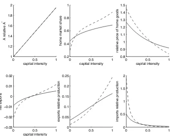
Figure 1.2: Heckscher-Ohlin case. The upper panels plot factor augmenting productivities against income per worker for the case of conditional factor price equalization. The lower panels show the case of multiple cones (= 0.5).
0 2 4 6 8
0 0.2 0.4 0.6 0.8 1 1.2 1.4 SGP CHE ITA AUTBEL JPN FRA DEUNLD NOR ESP FIN PRT DNK ISR ISL AUS USA HKGCAN IRL GBR SWE KOR GRC NZL TWN IRN TTO CYP CHL MYS HUNARG MUS
BRAVENMEXURY THA TUN DZAPAN BWA POL ECU TUR JAMPER COL ROM DOM CRI PRY JOR ZAF MAR IDNFJI CHNNIC BRB
LSOHNDZWE SLV PAK PHL LKAGTM COG PNG BOL EGY
NPLBGDIND CAFSYR ZMB
CMR KENBENSEN TGOMLI GMB NERGHA ZARMWISLERWAETHUGAMOZ
Income per worker
AH
0 2 4 6 8
0 2 4 6 8 10 12 SGP CHE ITA AUTBEL JPN FRAESPFINDEUNLDNOR PRT ISLAUSSWEHKGISRCAN IRLGBRDNK USA KORGRCNZL
TWN IRN TTO CYP CHL MYS HUNARG MUS
BRAVENMEXURY THA TUN DZA PAN BWA POL ECU TUR JAMPERCOL
ROM DOM CRI PRY JOR ZAF MAR IDNFJI CHN NIC BRB
LSOHNDZWE SLV PAKPHL LKA GTM COG PNG BOL EGY NPL IND BGD CAF SYR ZMB CMR KEN BEN SEN TGO MLI GMB NER GHA ZAR MWI SLE MOZ RWA ETH UGA
Income per worker
AK
0 2 4 6 8
0 0.2 0.4 0.6 0.8 1 1.2 1.4 SGP CHE ITA AUTBEL JPN FRA DEUNLD NOR ESP FIN PRT DNK ISR ISL AUS USA HKGCAN IRL GBR SWE KOR GRC NZL TWN IRN TTO CYP CHL MYS HUNARG MUS BRA VENMEXURY THA TUN DZAPAN BWA POL ECU TUR JAMPER COL ROM DOM CRI PRY JOR ZAF MAR IDNFJI CHN NIC BRB LSO ZWE HND SLV PAKPHL LKA GTM COG PNG BOL EGY
NPLBGDIND CAF
SYR
ZMB CMR
KENBENSEN TGOMLI GMB NERGHA ZARMWISLE
MOZ RWA ETHUGA
Income per worker
AH
0 2 4 6 8
0 1 2 3 4 SGP CHE ITA AUTBEL JPN FRADEU
NLDNOR ESP
FIN
PRT ISLISRDNKAUS USA HKG CAN IRL GBR SWE KOR GRC NZL TWN IRN TTO CYP CHL MYS HUN ARG MUS BRA VEN MEXURY THA TUN DZA PAN BWA POL ECU TUR JAMPER COL ROM DOM CRI PRY JOR ZAF MAR IDNFJI CHNNIC BRB LSO ZWE HND SLV PAK PHL LKAGTM COG PNG BOL EGY NPL IND BGD CAF SYR ZMB CMR KEN BENSEN TGO MLI GMB NERGHA ZAR MWI SLE MOZ RWA ETH UGA
Income per worker
input-output matrices, Bc =BU S. Then one can write the factor content of trade in
efficiency units as
Ff c∗ =DU S(I −BU S)−1(Xc−
X
c06=c
Mcc0).
Normalizing Af U S = 1 and dropping the equation for the US, the HOV equations
in efficiency units (1.24) form a system ofC−1 independent linear equations inAf c,
which can be solved for the unknown factor productivities.
From (1.25) we see that ifFf c∗ is small, relative productivities equal relative average products. In fact this is the case in the data if the factor content of trade is computed
with the US factor use matrix and as a consequence productivities computed with
Trefler’s method are similar to the ones obtained from (1.34), which also explains why
Trefler finds that relative productivities are similar to relative factor prices.29 Rich
countries are measured to have much higher human capital productivities than poor
nations, while poor countries tend to have higher productivities of physical capital.30
Example 3: Multiple Cones
If there are multiple cones of diversification, the picture is quite different because
the mapping between endowments, factor prices and factor productivities changes its
shape, depending on whether a country specializes or lies in a cone. Again, let us
take goods prices as parameters for now.
For countries that specialize in sector i∈ {H, K}the mapping from endowments,
factor prices and income to factor productivities looks similar to Caselli’s.
29Productivities are not reported, but very similar to figure 1.2. These results are robust to using the technology matrix of other countries as reference and to using the true input-output tables of each country in computing the factor content of trade.