CONTRASTING MAIN SELECTION METHODS IN GENETIC ALGORITHMS Alfonso H., Cesan P., Fernandez N., Minetti G., Salto C., Velazco L.
Proyecto UNLPAM-09/F0091
Departamento de Informática - Facultad de Ingeniería Universidad Nacional de La Pampa
Calle 110 esq. 9 – Local 14
(6360) General Pico – La Pampa – Rep. Argentina
e-mail: {alfonsoh,cesanp,fernaty,minettig,saltoc,velazcol}@ing.unlpam.edu.ar; Phone: (0302)22780/22372, Ext. 6412
Gallard R., Proyecto UNSL-3384032 Departamento de Informática Universidad Nacional de San Luis Ejército de los Andes 950 - Local 106
5700 - San Luis Argentina
E-mail: [email protected]
Phone: +54 652 20823 Fax : +54 652 30224
ABSTRACT
In genetic algorithms selection mechanisms aim to favour reproduction of better individuals imposing a direction on the search process. It does not create new individuals; instead it selects comparatively good individuals from a population and typically does it according to their fitness. The idea is that interacting with other individuals (competition), those with higher fitness have a higher probability to be selected for mating. In that manner, because the fitness of an individual gives a measure of its “goodness”, selection introduces the influence of the fitness function to the evolutionary process. Moreover, selection is the only operator of genetic algorithm where the fitness of an individual affects the evolution process. In such a process two important, strongly related, issues exist: selective pressure and population diversity. They are the sides of the same coin: exploitation of information gathered so far versus exploration of the searching space. Selection plays an important role here because strong selective pressure can lead to premature convergence and weak selective pressure can make the search ineffective [14]. Focussing on this equilibrium problem significant research has been done.
In this work we introduce the main properties of selection, the usual selection mechanisms and finally show the effect of applying proportional, ranking and tournament selection to a set of well known multimodal testing functions on simple genetic algorithms. These are the most widely used selection mechanisms and each of them has their own features.
A description of each method, experiment and statistical analyses of results under different parameter settings are reported.
KEYWORDS: Genetic algorithms, selection mechanisms, genetic diversity, premature convergence.
1 The Research Group is supported by the Universidad Nacional de La Pampa. 2
CONTRASTING MAIN SELECTION METHODS IN GENETIC ALGORITHMS 1. MAIN PROPERTIES OF SELECTION
By simulating evolution, a Genetic Algorithm (GA) maintain a population of multiple individuals (chromosomes) which evolve throughout generations by reproduction of the fittest individuals. After initialisation, to create the original population of individuals, a GA consists of a selection- recombination-mutation cycle until a termination criterion holds.
Selection, crossover and mutation are the main operators repeatedly applied throughout the GA execution used to modify individual features. So, it is expected that evolved generations provide better and better individuals (searchers in the problem space).
For the following discussion it is convenient to adopt the notation used by Bäck [6]. Let us call I the space of individuals a ∈ I and f : I →5 a real-valued fitness function. Let be µ the population size and P(t) = (a1t ..., aµ t) ∈Iµ a population at generation t.
A well known property of a selection operator is selective pressure which can be defined as the probability of the best individual being selected relative to the average probability of selection of all individuals.
It also can be seen as a parameter associated to the takeover time. The concept of takeover time is defined, in the work of Goldberg and Deb [12], as the number of generations necessary for a (unique) best individual found in the initial population to occupy the complete population by repeatedly applying a given selection mechanism alone [4]. If the takeover time is large or small then the selective pressure of a selection operator is, accordingly, weak (explorative search) or strong (exploitative search).
During the selection step of an EA copies of better ones replace worst individuals. Consequently, part of the genetic material contained in these worst individuals disappears forever. This loss of diversity is defined as the proportion of the population that is not selected for the next generation [7].
When the selection mechanism imposes a strong selective pressure then the loss of diversity can be high and, to prevent a premature convergence to a local optimum then, either a larger population size or adequate crossover and mutation operators are needed. On the other side of the coin a small selective pressure can excessively slow the convergence rate.
The population diversity was introduced by Bäck and Hoffmeister [3], in terms of the bias measure defined by Grefenstette [13] as follows;
− ⋅ =
∑
∑
∑
= = = = = µ µµ
1 1 , 0 1 , 1 , , ), 1 ( 1 )) ( ( t j i t j i a i t j i a i t j i l j a a max l t P bwhere l is the chromosome length and ati,j denotes the allele value. The bias b (0.5≤ b ≤ 1.0) indicates the average percentage of the most outstanding value in each position of the individuals. Smaller values of b indicate higher genotypic diversity and vice versa. The bias b can be used to formulate an adequate termination criterion.
The selection probability Psel is an important parameter of a selection mechanism and normally determines the number of expected copies of an individual after selection given by:
)
(
)
(
a
it= µ
⋅
P
sela
itξ
These expected values not always agree with the algorithmic sampling frequencies. Different algorithms provide large or minor differences between them. Baker [2] introduced the concept of
bias as an individual’s actual sampling probability and its expected value. Also he defined spread
as the range of possible values for the number of copies an individual receives by a selection mechanism.
Two related properties are selection intensity and growth rate.
σ
/
)
(
f
beforef
afterI
=
−
where σ is the mean variance of the population before selection.
For quasi normal distributed values of individual’s fitness in the population, I gives a measure of the average fitness of the selected individuals and that of the whole population [15], [5].
The growth rate is defined as the ratio of the number of the best solutions in two consecutive generations. Early and late growth rates are calculated respectively, when the proportion of best solution is not significant, at the beginning, and large (about 50%) in the final stage of the evolution process. Both can be used as measures of convergence for fast near-optimizers or precise-optimizer algorithms.
From the above discussion we can conclude that a selection mechanism should be the driving force to conduct the search towards better individuals but also it is concerned of maintaining a high genotypic diversity, to avoid stagnation. Can we ask only to selection to fulfil this compromise? As stated by Deb ([12]):
“... for a successful EC simulation, the required selection pressure of a selection operator depends on the recombination and mutation operators used. A selection scheme with a large selection pressure can be used, but only with a highly disruptive recombination and mutation operators.” Conversely, when a recombination scheme forces the exploitation in the searching space, then alternative selection mechanisms should be used [10 ].
2. COMMONLY USED SAMPLING MECHANISMS
Most of the topics of this section can be found in more detail in chapter 5 the Bäck book [6]. For the following discussion we concentrate on GAs applied to search (optimization) problems. Within this framework we refer to the fitness function f, as a mapping which maps the value of the objective function to an interval in ℜ+. In that way maximization and minimization are equivalent.
Proportional Selection
In proportional selection, an individual ai is chosen at random for mating from a population of size
µ according to the following probability:
∑
= = µ
1
) (
) ( )
(
j j i i
sel
a f
a f a
P
This is the simplest selection scheme also known as roulette-wheel selection or stochastic sampling with replacement.
Here, individuals are mapped to contiguous segments in the real interval [0,1] in such a way that a segment corresponding to an individual has a size equal to the individual fitness. Then a random number in such interval is generated and the individual whose segment encompasses the random number is selected.
One pernicious consequence of this assignment of probabilities resides in the different behaviour showed by the EA for functions that are equivalent from the optimization point of view such as
f(x) = ax2 and g(x) = ax2 + b. For example, if for certain values of x, it results b >>ax2 then the selection probabilities of many individuals would be extremely similar and the selective pressure would result too weak. Consequently optimization of g(x) becomes a random search process. This frequently happens when the population converges to a narrow range of values during the evolution process.
To avoid this undesirable behaviour the fitness function can be scaled to the worst individual and instead of absolute individual’s fitness, we manage with an individual’s fitness relative to the worst individual.
But on the other hand, when scaling to the worst individual, the inverse effect (excessive selective pressure) can emerge inasmuch as a super-performer appears in the population. Copies of this super-individual will rapidly invade the whole population.
function being optimized. Different categories of scaling were defined. Goldberg introduced;
linear, sigma truncation and power law scaling [11] and Michalewicz extended the later to another method knew as non-uniform scaling [14].
Goldberg and Deb [12] determined the takeover time τ for f1(x) = xc and f2(x) = exp(cx):
c c f f / ) ln ( / ) 1 ln ( 2 1 µ µ τ µ µ τ ≈ − ≈ ∗ ∗
This results tell us that the takeover time for proportional selection is of the order of Ο(µ ln µ), regardless of a polynomial or exponential objective function in x.
As asserted in [14], considerable effort has been done in the search for a trade-off between population diversity and selective pressure. In that direction, one of the originally most recognized works was due to De Jong [9] who introduced several variations of proportional selection. The first one, the elitist model, preserves indefinitely the best-found individual. The second modification, the
expected value model, attenuates the stochastic errors by introducing a count, associated to each individual, which is decreased each time it is selected for reproduction. The third variation, the
elitist expected value model, combines the first two variations. In the fourth variation, the crowding value model, a newly created individual replaces an old one, which is selected from those resembling the new one.
Brindle [8] and Baker [2] considered further modifications, remainder stochastic sampling and
stochastic universal sampling, that were confirmed as improvements over the simple selection mechanism.
Rank-based selection
The need of scaling procedures under proportional selection might induce Baker to consider an alternative sampling mechanism, to control the EA behaviour [1]. The first approach was called
linear ranking.
By means of linear ranking the selective pressure can be controlled more directly than by scaling and consequently the search process can be accelerated remarkably. During many years this method was criticized due to the apparent inconsistency with the schema theorem, which affirms that low order, above average fitness schemata receive exponentially increasing trials in subsequent generations. Nevertheless, Whitley [16] pointed out that ranking acts as a function transformation assigning new fitness value to an individual based on its performance relative to other individuals. Why to insist that “exact fitness” should be used? He posed.
The Baker’s original linear ranking method assigns a selection probability that is proportional to the individual’s rank. Here, according to Bäck [6] the mapping rank: I→{1,...,µ} is given by:
{
}
{
1,..., 1}
: ( ) ( ) ) ( : ,..., 1 1 + ≤≥ − ∈ ∀ ⇔ = ∈ ∀ j j i a f a f j i a rank i µ µwhere ≤≥ denotes the ≤ relation or the ≥ relation for minimization or maximization problems res-pectively. Consequently the index i of an individual ai denotes its rank. Hence, individuals are sorted according to their fitness resulting a1 the best individual and aµ the worst one. Assuming that the expected value for the number of offspring to be allocated to the best individual is ηmax =µP(a1) and that to be allocated to the worst one is ηmin =µP(aµ) then
( )
−
−
⋅
−
−
=
1
1
)
(
1
µ
η
η
η
µ
i
a
P
sel i max max minAs the following constraints must hold
i a
∑
==
µ 11
)
(
i i sela
P
it is required that:
max min
max
η
η
η
≤ = −≤ 2 and 2
1
The selective pressure can be adjusted by varying ηmax. As remarked by Baker if ηmax = 2.0 then all individuals would be within 10% of the mean and the population is driven to convergence during every generation. To restrain selective pressure, Baker recommended a value of ηmax =1.1. This value for ηmax close to 1 leads to Psel (ai) ≅ 1/µ , almost the case of random selection.
Goldberg and Deb also determined the takeover time for two cases of linear ranking: ηmax = 2.0 and 1<ηmax < 2.
(
)
(
1)
ln 1 2 ln log log 2 , 1 2 2 2 − − ≈ + ≈ ∗ ∗ µ η τ µ µ τ max andA ranking mechanism can be devised also by means of non-linear mappings. For instance Michalewicz, to increase selective pressure, has used an exponential ranking approach where the probabilities for selection were defined as follows:
1 0 with , ) 1 ( )
( = − −1 < <<
c c
c a
Psel i i
where the constant c, assigns the probability of selection for the best individual.
As pointed by Michalewicz [14], even though ranking methods have shown, in some cases, to effectively improve genetic algorithms behaviour some apparent drawbacks remain. They can be summarized as follows: the responsibility to decide when to use these mechanism is put on the user’s hands, the information about relative evaluation of chromosomes is ignored, all cases are treated uniformly regardless of the magnitude of the problem and, finally, the schema theorem is violated.
Tournament Selection
In tournament selection q individuals are randomly chosen from the population and then the best fitted individual, designated as the winner, is selected for the next generation. The process is repeated µ times, until the new population is completed.
The parameter q is known as the tournament size and usually it is fixed to q = 2 (binary tournament). If q = 1 then there is no selection at all: each individual has the same probability to be selected. As long as q increases the selective pressure is augmented.
As Brickle [7] affirms, tournament selection can be implemented efficiently having the time complexity O(µ) because no sorting of the population is necessary but, as a counterpart, this also leads to high variance in the expected number of offspring resultant from µ independent trials. As scaling techniques needed for proportional selection are unnecessary, the application of the selection method is as well simplified. Furthermore, global calculations to compute the reproduction rates of individuals are needless under this method.
As showed by Bäck [6], the selection probability for individual ai , (i ∈ {1,...,µ} ) for q-tournament
selection is given by
(
) (
)
(
q q)
q i
sel
a
i
i
P
=
µ
−
+
−
µ
−
µ
1
1
)
(
(
ln ln(ln ))
ln 1µ
µ
τ
∗ ≈ + q q3. EXPERIMENTAL TESTS
Here we describe an approach to contrast results obtained from optimization of recommended multimodal testing functions when either proportional, ranking and tournament selection mechanisms are applied on a simple GA.
For our experiments, 20 runs with randomised initial population of size fixed to 80 individuals were performed on each function, using binary coded representation, elitism, one point crossover and bit flip mutation. . The number of generations was variable and probabilities for crossover and mutation were fixed to 0.65 and 0.001 for f1 and f2 and 0.50 and 0.005 for f3 and f4. In order to isolate the convergence effect of each selection method, the kind of genetic operators and parameter settings chosen were those commonly used in optimising with a simple GA.
For this report, we choose contrasting results on four well-known multimodal testing functions of varying difficulty:
f1: Michalewickz’s multimodal function
f2: Michalewickz’s highly multimodal function
850292 . 38 : 8 . 5 1 . 4 , 1 . 12 0 . 3 ; , 20 ) 4 ( 5 . 21 , 2 1 2 2 1 1 2
1
)
(
)
(
value maximum estimated forx
x
x
sin
x
x
sin
x
x
x
f
≤ ≤ ≤ ≤ − + + =⋅
π
⋅
⋅
π
⋅
f3: Branins's Rcos Function
(
)
(
)
f
x x
x
x
x
minimum4 1 2
2 2
2
1 1 1
1
5 1
4
5
6 10 1 1
8 10
5 10 0 15
0 397887
(
,)
. cos( ) ,: , : ;
: .
= x
x
x
= global value 2 2 − ⋅ ⋅ + ⋅ − + ⋅ − ⋅ + − =
⋅
π π πf4: Griewangk's Function F8
f
x
x
x
x
i i i i i im i n i m u m g l o b a l v a l u e
1
2
1 5
1
4 0 0 0
6 0 0 6 0 0 1 5
0 0
(
)
c o s ,: : ;
: .
+
, i
i = 1 5 = − = − =
∑
∏
=As an indication of the performance of the algorithms the following relevant variables were chosen:
Ebest = ((opt_val - best value)/opt_val)100
It is the percentile error of the best found individual when compared with the known, or estimated, optimum value opt_val. It gives us a measure of how far are we from that opt_val.
Epop = ((opt_val- pop mean fitness)/opt_val)100
It is the percentile error of the population mean fitness when compared with opt_val. It tell us how far the mean fitness is from that opt_val.
4. RESULTS
The main selection mechanisms were applied on each function. Proportional selection was applied in the conventional way, and it is denoted by SGA in the figuresand tables. In the case of raking selection settings for low, intermediate and high values of ηmax were used: 1.1, 1.5 and 2.0 respectively. In the case of tournament selection the size q of the set of competing individuals was set to 2, 3, 4, 5, 10 and 20.
In the analysis of each function we show those results of ranking and tournament corresponding to the setting of parameters for which the method behaves better.
In the following tables µperfvar,σ perfvar,σ/µ perfvar stands for the mean, standard deviation and
coefficient of deviation of the corresponding performance variable (perfvar)
Function f1
For the multimodal Michalewicz’s function using ranking the best mean Ebest values
where
found with
ηmax = 2.0. Poor results with values as high as 32% were obtained with remaining settings. In the case of tournamentthe best mean
Ebest
values where found with
q = 4, and remaining settings produced values in the range 0.9% to 5.5%.In many runs under any of the alternative selection mechanisms the genetic algorithm
reached the optimum.
Following figures and tables discuss on results for
f1
Ebest
0 5 10 15 20
1 4 7 10 13 16 19
[image:7.612.91.524.361.757.2]Propor Rank 2.0 Tourn (q=4)
Fig. 1: Ebest values throughout the experiments for Propor, Rank and Tourn on
f1
65 80 75
35
20 25
0 20 40 60 80 100
Ebest< 1% Ebest >= 1%
Propor
Rank 2.0 Tourn (q=4)
Fig 2. Percentile of Ebest values bellow and above 1% throughout
the experiments for Propor, Rank and Tourn on
f1
µµ
Ebestσσ
Ebestσσ
Ebest/
µµ
EbestPropor
2,17438421
4,1829588
1,9237441
Rank 2,0
0,81565754
2,3491819
2,88010812
Tour (q=4)
0,9395669
2,3493265
2,50043554
Figures 1 and 2, and table 1 show that best values are found with Rank (2.0) where 80% of the Ebest values are less than 1%. Also with Tourn (q=4) good results are obtained. In this case 75% of the Ebest values are less than 1%.
Both selection mechanism outperform proportional selection. Nevertheless, as can be observed in figure 1, under any selection mechanism the algorithm reach sometimes the optimum. Also it can be observed that statistical values are moderately dispersed around the mean.
Analysis of Epop follows.
Epop
0 5 10 15 20
1 4 7 10 13 16 19
[image:8.612.87.523.211.620.2]Propor Rank 2.0 Tourn (q=4)
Fig. 3: Epop values throughout the experiments for Propor, Rank and Tourn on
f1
60 70 65
40
30 35
0 20 40 60 80 100
Epop < 1% Epop >= 1%
Propor
Rank 2.0 Tourn (q=4)
Fig 4. Percentile of Epop values bellow and above 1% throughout
the experiments for Propor, Rank and Tourn on
f1
µµ
Epopσσ
Epopσσ
Epop/
µµ
EpopPropor
2,6557993
4,4210455
1,66467603
Rank 2.0
1,15964994
2,4066567
2,07533038
Tourn (q=4)
1,10501227
2,3066101
2,08740683
Table 2: Mean and standard deviation for Epop throughout
the experiments for Propor, Rank and Tourn on
f1
Function f2
Function f2 was definitively harder than f1 for the genetic algorithm. For the highly multimodal Michalewicz’s function using ranking the best mean Ebest values where found with ηmax = 2.0. Poor results with values as high as 30% were obtained with remaining settings.
In the case of tournament the best mean Ebest values where found with q = 3, and remaining settings produced values in the range 5.8% to 6.4%.
In few runs under any of the alternative selection mechanisms the genetic algorithm reached the optimum.
Ebest
0 5 10 15
1 4 7 10 13 16 19
[image:9.612.95.515.152.569.2]Propor Rank 2,0 Tourn (q=3)
Fig. 5: Ebest values throughout the experiments for Propor, Rank and Tourn on
f2
85
80 90
15 20 10
0 20 40 60 80 100
Ebest< 8% Ebest >= 8%
Propor
Rank 2,0
Tourn (q=3)
Fig. 6: Percentile of Ebest values bellow and above 8% throughout
the experiments for Propor, Rank and Tourn on
f2
µµ
Ebestσσ
Ebestσσ
Ebest/
µµ
EbestPropor
3,43027374
3,2560932
0,94922255
Rank 2,0
4,77518358
3,8557875
0,80746372
Tourn (q=3)
4,24364967
3,0211970
0,71193366
Table 3: Mean and standard deviation for Ebest throughout
the experiments for Propor, Rank y Tourn on
f2
Analisys of Epop follows.
Epop
0 5 10 15
1 4 7 10 13 16 19
[image:10.612.92.517.110.520.2]Propor Rank 2,0 Tourn (q=3)
Fig. 7: Epop values throughout the experiments for Propor, Rank and Tourn on
f2
65
55 60
35 45
40
0 20 40 60 80 100
Epop < 5% Epop >= 5%
Propor
Rank 2,0 Tourn (q=3)
Fig. 8: Percentile of Epop values bellow and above 5% throughout
the experiments for Propor, Rank and Tourn on
f2
µµ
Epopσσ
Epopσσ
Epop/
µµ
EpopPropor
4,69946624
3,0872195
0,65692983
Rank 2,0
5,01799048
3,7930008
0,75588043
Tourn (q=3)
4,44483845
3,0806361
0,69308169
Table 4: Mean and standard deviation for Epop throughout
the experiments for Propor, Rank and Tourn on
f2
Function f3
For the Branin’s function using ranking the best mean Ebest values where found with ηmax = 2.0. Good results with values of 0.88% and 0.23% were obtained with ηmax = 1.1 and ηmax = 1.5, respectively.
In the case of tournament the best mean Ebest values where found with q = 4, and remaining settings produced also good values in the range 0.02% to 0.03%.
In many runs under any of the alternative selection mechanisms the genetic algorithm reached the optimum.
Following figures and tables discuss on results for
f3
.
Ebest
0 0,5 1 1,5
1 4 7 10 13 16 19
[image:11.612.93.516.179.616.2]Propor Rank 2,0 Tourn (q=4)
Fig. 9: Ebest values throughout the experiments for Propor, Rank and Tourn on
f3
80 100 100
20
0 0
0 20 40 60 80 100
Ebest< 0,01% Ebest >= 0,01%
Propor Rank 2,0
Tourn (q=4)
Fig. 10: Percentile of Ebest values bellow and above 0,01% throughout
the experiments for Propor, Rank and Tourn on
f3
µµ
Ebestσσ
Ebestσσ
Ebest/
µµ
EbestPropor
0,06332596
0,2468112
3,89747293
Rank 2,0
0,00239591
0,0001668
0,06960991
Tourn (q=4)
0,00236471
0,0001263
0,05339067
Table 5: Mean and standard deviation for Ebest throughout
the experiments for Propor, Rank and Tourn on
f3
Analisys of Epop follows.
Epop
0 1 2 3 4 5
1 4 7 10 13 16 19
[image:12.612.92.523.76.515.2]Propor Rank 2,0 Tourn (q=4)
Fig. 11: Epop values throughout the experiments for Propor, Rank and Tourn on
f3
45 40
70
55 60
30
0 20 40 60 80 100
Epop < 0,01% Epop >= 0,01%
Propor Rank 2,0
Tourn (q=4)
Fig. 12: Percentile of Epop values bellow and above 0,01% throughout
the experiments for Propor, Rank and Tourn on
f3
µµ
Epopσσ
Epopσσ
Epop/
µµ
EpopPropor
0,19628763
0,5751949
2,93036747
Rank 2,0
0,75882468
1,0576247
1,3937669
Tourn (q=4)
0,30620344
0,7459909
2,43625917
Table 6: Mean and standard deviation for Epop throughout
the experiments for Propor, Rank and Tourn on
f3
Function f4
For the Griewangk's function using ranking the best mean Ebest values where found with ηmax = 2.0.
Poor results with values as high of 48% and 39% were obtained with ηmax = 1.1 and ηmax = 1.5, respectively.
In the case of tournament the best mean Ebest values where found with q = 20, and remaining settings produced values in the range 0.14% to 5.8%.
In few runs under any of the alternative selection mechanisms the genetic algorithm reached the optimum.
Following figures and tables discuss on results for f4.
Ebest
0 1 2 3 4 5
1 4 7 10 13 16 19
[image:13.612.90.513.194.609.2]Propor Rank 2,0 Tourn (q=20)
Fig. 13: Ebest values throughout the experiments for Propor, Rank and Tourn on f4.
5 70
35
95
30 65
0 20 40 60 80 100
Ebest< 0,1% Ebest >= 0,1%
Propor
Rank 2,0
Tourn (q=20)
Fig. 14: Percentile of Ebest values bellow and above 0,1% throughout
the experiments for Propor, Rank and Tourn on
f4
µµ
Ebestσσ
Ebestσσ
Ebest/
µµ
EbestPropor
1,4864597
1,2129254
0,81598273
Rank 2,0
0,08496272
0,0720580
0,84811291
Tourn (q=20)
0,14493713
0,0999323
0,68948752
Table 7: Mean and standard deviation for Ebest throughout
the experiments for Propor, Rank and Tourn on
f4
The above figures and table show a better performance of the algorithm under ranking selection. With tournament have an intermediate performance and the worst is achieved by means of the conventional proportional selection. This can be clearly seen in figure 13.
Epop
0 10 20 30 40 50
1 4 7 10 13 16 19
[image:14.612.97.512.36.444.2]Propor Rank 2,0 Tourn (q=20)
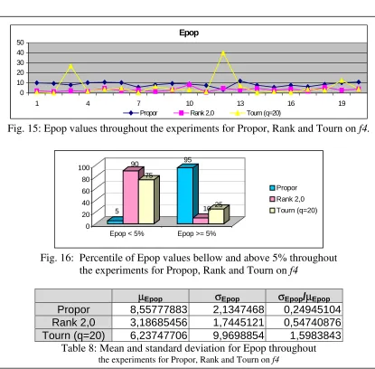
Fig. 15: Epop values throughout the experiments for Propor, Rank and Tourn on
f4.
5 90
75
95
10 25
0 20 40 60 80 100
Epop < 5% Epop >= 5%
Propor
Rank 2,0 Tourn (q=20)
Fig. 16: Percentile of Epop values bellow and above 5% throughout
the experiments for Propop, Rank and Tourn on
f4
µµ
Epopσσ
Epopσσ
Epop/
µµ
EpopPropor
8,55777883
2,1347468
0,24945104
Rank 2,0
3,18685456
1,7445121
0,54740876
[image:14.612.96.516.54.168.2]Tourn (q=20)
6,23747706
9,9698854
1,5983843
Table 8: Mean and standard deviation for Epop throughout
the experiments for Propor, Rank and Tourn on f4
The above figures and table shows again that the mean population fitness is nearer to
that of the optimum under ranking or tournament when contrasted with proportional
selection.
GBEST
A
NALYSISµµ
Gbestσσ
Gbestσσ
Gbest/
µµ
GbestPropor
207,15
90,6097909
0,43741149
f1
Rank 2.0
129,40
72,7174778
0,56195887
Tourn (q=4)
109,15
78,5522119
0,71967212
Propor
241,65
79,4091835
0,32861239
f2
Rank 2,0
82,75
32,7219144
0,39543099
Tourn (q=3)
81,10
30,8389706
0,38025858
Propor
565,90
269,4237320
0,47609778
f3
Rank 2,0
199,25
187,6805447
0,94193498
Tourn (q=4)
366,85
352,2036305
0,96007532
Propor
550,30
344,3280413
0,62570969
f4
Rank 2,0
635,85
273,6550412
0,43037673
[image:14.612.91.528.558.747.2]Table 9: Mean, Standard deviation and coefficient of deviation values for Gbest throughout the experiments on each function under each approach
Except for
f4,
table 9 clearly shows that the best individual, retained by elitism, is found
in a much earlier generation when we use either ranking or tournament selection.
5. CONCLUSIONS
This paper presented discussed the main properties of selection methods widely used in evolutionary computation. A set of experiments on a selected set of multimodal testing functions of varying difficulty was described.
At the light of the results we can conclude that even though proportional selection is the most diffused method of selection, similar or better quality of results can be obtained with ranking and tournament selection when the issue is to optimize multimodal functions.
Nevertheless this requires an extra effort: tunning of parameters. In our case, extensive experimental work was necessary to determine the best setting for each particular function. Those setting found a better balance between selective pressure and genetic diversity.
Today a new trend exists in evolutionary computation which attempt to modify parameters settings “on the fly”, while the algorithm is executing.
Future work will consider incorporation of some feedback from the evolution process itself to dynamically adjust parameter settings.
6. ACKNOWLEDGEMENTS
We acknowledge the cooperation of the project group for providing new ideas and constructive criticisms. Also to the Universidad Nacional de San Luis, the Universidad Nacional de La Pampa , the CONICET and the ANPCYT from which we receive continuous support.
7. REFERENCES
[1] Baker J. E.:Adaptive selection methods for genetic algorithms. . Proc. Of the 1st International Conf. On Genetic Algorithms and Their Applications, pp 101-111. Lawrence Erlbaum Associates, 1985.
[2] Baker J. E.: Reducing bias and inefficiency in the selection algorithm. Proc. Of the 2nd International Conf. On Genetic Algorithms, pp. 14-21. J.J Grefenstette Ed, 1987.
[3] Bäck T., Hoffmeister F.: Extended selection mechanisms in genetic algorithms. Proc. of the 4th Int. Conf. on Genetic Algorithms, pp 92-97, Morgan Kaufmann, 1991.
[4] Bäck T.: Selective pressure in evolutionary algorithms: a characterization of selection mechanisms. Proc. 1st IEEE Conf. On Evolutionary Computation (Orlando, FL, 1994) (Piscataway, NJ: IEEE) pp 57-62.
[5] Bäck T: Generalised convergence models for tournament and (µ,λ)-selection. Proc. Of the 6th International Conf. On Genetic Algorithms. Morgan Kaufmann 1995.
[6] Bäck T: Evolutionary algorithms in theory and practice. Oxford University Press, 1996. [7] Blickle T. and Thiele, L.: A comparison of selection schemes used in genetic algorithms.
Technical Report 11 TIK, Swiss Federal Institute of Technology, December 1995.
[8] Brindle A.: Genetic algorithms for function optimization. Doctoral Dissertation. University of Alberta, Edmonton, 1981.
[9] De Jong K. A.: An analisis of the behavior of a class of genetic adaptive systems. Doctoral dissertation, University of Michigan. Dissertation abstract International, 36(10), 5140B. (University Microfilms no 76-9381).
[11] Goldberg, D.E. Genetic Algorithms in Search, Optimization and Machine Learning. Addison-Wesley, Reading, MA. (1989).
[12] Goldberg D. E. And Deb K.: A comparison of selection schemes used in genetic algorithms. Foundations of Genetic Algorithms I . Morgan Kaufmann, pp 69-93.
[13] Grefenstette J.J.: A user’s guide to GENESIS. Navy Center for Applied Research in Artificial Intelligence, Washington D.C., 1987.
[14] Michalewicz, M.: Genetic Algorithms + Data Structures = Evolution Programs. Springer, third revised edition, 1996.
[15] Mühlenbein H., Schlierkamp-Voosen D.: The science of breeding and its application to the breeder genetic algorithm (BGA). Evolutionary Computation 1(4), pp 335-360.