ADAPTIVE SPACE-TIME FINITE ELEMENT METHODS FOR
ACOUSTICS SIMULATIONS IN UNBOUNDED DOMAINS
PACS REFERENCE: 43.20.Px Thompson, Lonny; He, Dantong
Clemson University, Department of Mechanical Engineering Clemson, South Carolina 29634-0921 USA
(864)656-5631
email: [email protected]
ABSTRACT
High-order accurate and unconditionally stable time-discontinuous methods are implemented with nonreflecting boundary conditions in an adaptive space-time finite element method for acoustic radiation and scattering problems in exterior domains. Anh-adaptive space-time procedure based on theZ2 error estimate and the superconvergent patch recovery (SPR) technique, together with a temporal error estimate arising from the discontinuous jump in solution between time steps is used to maintain accuracy within a prescribed tolerance and drive dynamic mesh distributions. Error estimates of the nonreflecting boundaries are also monitored in the solution process. A new superconvergent interpolation method is developed for projection between adaptive meshes. Numerical studies of time-dependent scattering from an ellipse demonstrate the efficiency and reliability gained from the adaptive solution.
Introduction
We describe recent advances in the development of high-order accurate and unconditionally stable space-time methods which employ finite element discretization of the time domain as well as the usual discretization of the spatial domain. In particular, we examine the implementation of a sequence of high-order accurate radiation boundary conditions [1, 2, 3, 4] in an adaptive space-time finite element method for acoustic radiation and scattering problems in exterior domains. In particular, a multi-field discontinuous Galerkin finite element method (DGFEM) is used with independent acoustic pressure and velocity variables, [5, 6]. A multi-level iterative scheme is used to solve the resulting fully-discrete system equations for the interior hyperbolic equations coupled with the first-order temporal equations associated with auxiliary functions in the nonreflecting boundary conditions. The iterative strategy requires only a few iterations per time step to resolve the solution to high accuracy. Anh-adaptive space-time strategy is employed based on the Zienkiewicz-Zhu [7] spatial error estimate using the superconvergent patch recovery (SPR) technique, together with a temporal error estimate arising from the discontinuous jump in velocity and pressure between time steps. As sound pulses propagate throughout the mesh, elements are refined near wave fronts, and unrefined where the solution is smooth or quiescent. Time-steps are also adjusted to maintain given error tolerances. Errors in the time integration of the auxiliary functions in the nonreflecting boundary conditions are also monitored and maintained within a tolerance. Numerical studies of transient scattering demonstrate the reliability and efficiency gained from the adaptive strategy.
Two-Dimensional Wave Equation on Unbounded Domains
We consider time-dependent waves in an infinite two-dimensional regionR ⊂R2, surrounding an object with surfaceS.
Within Ω, the solution u(x, t) : Ω×R+7→R, satisfies the scalar wave equation,
1
c∂tv = ∇
2u+ f(x, t), v=1
c∂tu, x∈Ω, t∈R
R
S D
Γ Ω
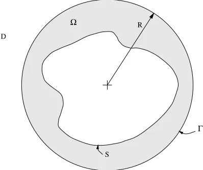
Figure 1: Illustration of two-dimensional un-bounded region R surrounding a scatterer S. The computational domain Ω⊂ Ris surrounded by a circular truncation boundary Γ of radiusR, with exterior region D=R −Ω.
with initial conditions, u(x,0) = u0(x), v(x,0) = v0(x). On the scatterer, we can specify a Neumann boundary condition,∂nu=g(x, t),x∈ S, t∈R+.
We denote the solution evaluated on the circular truncation boundary at r=Rby,
uΓ(θ, t) =u(R, θ, t), vΓ(θ, t) =1
c∂tuΓ, θ∈[0,2π), t∈R
+, (2)
Letw(θ, t) ={wj(θ, t)}pj=1, be defined as a time-dependent vector of real valued scalar auxiliary functions, i.e.,w= (w1, w2,· · ·, wp). We can expand the auxiliary functionsw(θ, t) and solution on the truncation boundaryuΓ(θ, t) by a Fourier series,
uΓ(θ, t) =
∞
X
m=−∞
um(t) eimθ, w(θ, t) =
M
X
m=−M
wm(t) eimθ (3)
with complex-valued Fourier modesum(t) :R+7→C, andwm(t) ={wmj }pj=1,wm,j(t) :R+ 7→C,
defined by the tangential Fourier transform:
um(t) = 1 2π
Z 2π
0
uΓ(θ, t) e−imθdθ, wm(t) = 1
2π
Z 2π
0 w
(θ, t) e−imθdθ. (4)
Hereum=u∗−m, andwm=w∗−m, with the asterisk denoting the complex conjugate, andi=√−1.
Using this expansion, we then approximate the exterior impedance on Γ, by the sequence of high-order accurate radiation boundary conditions derived in [4]:
∂ru|r=R+vΓ(θ, t) + 1
2RuΓ(θ, t) =
N
X
m=−N
wm1(t) eimθ (5)
wm0 (t) +Amwm(t) =bmum(t), wm(0) = 0 (6)
In the above, the prime indicates a derivative;wm(t) are time-dependent vector functions of order
p, and Am ={Aijm}pi,j=1, is a tri-diagonal matrix for each mode m, see [4]. The constant vector bm={bjm}pj=1 is defined bybm=8Rc2(1−4m2)e1.
Discontinuous Galerkin FEM
The development of the space-time method proceeds by considering a partitionMof the total time interval,t∈J = (0, T),0< T <∞, intoN time steps{In}nN=0given byIn={(tn, tn+1)}Nn=0. The length of the variable time step is given by ∆tn =tn+1−tn. Using this notation,Qn = Ω×In, are thenth space-time slabs. Within each space-time slab, the spatial domain is subdivided into
Dn elements. We define the jump operator across space-time slabs as,
[[u(tn)]] = u(x, t+n)− u(x, t−n), 0≤n≤N
[image:2.612.93.292.45.212.2]tn,1 t n tn tn+1 In,1 In t0 x2 x 1 ,0 0 Q e n Q e n,1 Qn n
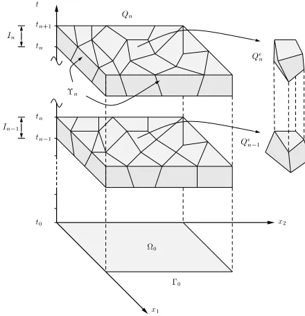
Figure 2: Illustration of two consecutive space-time slabs Qn−1 and Qn, each with different meshes. Within each space-time element, the trial solution and weighting function are approximated by a finite basis which depend on both spatial x, and tem-poral t, dimensions. The basis functions are assumed C0(Qn) continuous through-out each space-time slab, but are allowed to be discontinuous across the interfaces of the slabs. The space of finite element basis functions in our multi-field representation is stated in terms of independentvariables
u, andv.
The statement of the time-discontinuous Galerkin method may be stated as
Given: Load dataf , g, and initial conditions{u(x, t−n), v(x, t−n)},wm(t−n), from the previous time
step, then for each space-time slab, n= 0,1, . . . , N−1;Find: u={u(x, t), v(x, t)}, and wm(t),
x∈Ω∪∂Ω, t∈In = (tn, tn+1), such that for all admissible functions ¯u={u¯(x, t),v¯(x, t)}, and ¯
wm(t),m∈(−M, M), the following coupled integral equations are satisfied,
A( ¯u,u)n+BΓ( ¯u,u)n=FS(¯v)n+FΓ(¯v, w1m) (7)
Am( ¯wm,wm)n=Fm( ¯wm1, um), m∈(−M, M) (8)
with
A( ¯u,u)n := Z
In
(¯v , ∂tv) + (∇v ,¯ ∇u) + (∇u ,¯ 1
c∇∂tu− ∇v)
dt
+ (¯v(t+n),[[v(tn)]]) + (∇u¯(t+n),[[∇u(tn)]])
BΓ( ¯u,u)n := Z
In
2R(¯v , v)Γ+ (¯v , u)Γ+ (¯u , 1
c∂tu−v)Γ
dt+ (¯u(t+n),[[u(tn)]])Γ
Am( ¯wm,wm)n :=
Z
In
{w¯m(t)·wm0 (t) + ¯wm(t)·Amwm(t)} dt+ ¯wm(t+n)·[[wm(tn)]]
Fm( ¯wm1, um) := b1m
Z
In
¯
w1m(t)um(t) dt
FΓ(¯v, w1m) := 2R
M
X
m=−M
Z
In
(¯v ,eimθ)Γwm1(t) dt
On a typical current time slabIn = (tn, tn+1) = (t1, t2), with length ∆tn =t2−t1 >0, and temporal approximation orderr, the DGFEM is found by solving the coupled variational problem (7)-(8). The sourcef(x, t), Neumann datag(x, t), initial conditions from the previous time-step
{u(x, t−n), v(x, t−n)}, andwm(t−n), are the known data on the time slab. Coupling occurs through
driverswm(t) on the right-hand-side of Eq. (7), and boundary modesum(t), defined by (4) on the
right-hand-side of (8).
Space-Time Discretization of the Hyperbolic Wave Equation
In this paper, within a space-time slab,Qn = Ω×In, we assume an orthogonal space-time dis-cretization with linear temporal approximation,
u(x, t) = 2 X
i=1
uhi(x)φi(t) =Nn(x) 2 X
i=1
[image:3.612.94.314.46.274.2]where {φi}2i=1 are basis functions of P1(In). These basis functions may be high-order spec-tral, defined by continuous Lagrange interpolation, or p-version, defined by hierarchical Legendre polynomials. The FE approximations of {ui} are given as linear combinations of basis func-tions NA, and di = {uA(ti)}DA=1n . The solution at the bottom is denoted, t1 = t+n, and top,
t2 = t−n+1, the initial condition from the previous step is denoted t0 = t−n = t+n−1. Similarly,
v(x, t) =P2i=1vhi(x)φi(t) =Nn(x)P2i=1φi(t)ci.The time-dependent auxiliary functions
approx-imated by,
wm(t) =
2 X
i=1
wm,iφi(t) (10)
Substituting the space-time approximations into the space-time variational equations results in the fully discrete matrix problem,
ˆ
M M12ˆ ˆ
M21 Mˆ c1 c2
=
ˆ r1
ˆ r2
(11)
where ˆM =M +∆4tC. M12ˆ and ˆM21 depend on the the mass,damping,and stiffness matrices M,C,K. The rhs vectors are functions of: ˆri = ri(fi,c0,M,K,∆t), The displacements are
simply updated with,
d1=d0+∆t
6 (c1−c2), d2=d0+ ∆t
2 (c1+c2) (12)
d0 =d(t−n), and c0 =c(t−n) are initial conditions from the previous time-step. The load vectors do to the coupling from the auxiliary functionw1m(t) are given by,
fjΓ = 2R M
X
m=−M
w1m,jFm, Fm={FAm}, FAm:= (NA, eimθ)Γ
The time discretization for the first-order boundary equations takes the form,
I −(I+∆3tAm)
3(−I+∆3tAm) I
wm,1 wm,2
= ˆ
fm,1 ˆ fm,2
(13)
where the rhs vectors are driven bywm(t−n), and the modesum,j,
um(t) = 2 X
i=1
um,jφi(t), um,j = 1
πF ∗
m,n·dj (14)
A remarkable feature of this form is that for spectral interpolation in space, nodal quadrature may be used to diagonalize bothM andC, resulting a diagonal mass matrix and complete decoupling of the equations of the upper and lower sub-block diagonals. In this case, each time step requires only matrix-vector products with ˆM12 at each iteration in the solution for c1 and c2. Wiberg and Lee [8] derived a different form, with ˆM = M + ∆2tC + ∆6tK; this submatrix cannot be convieniently diagonalized because of the presence ofK.
The orderpused in the radiation boundary is typically less thanp <10, resulting in relatively small matricesAm. The number of modesm∈(−M, M) included depends on the complexity of the
solution as measured by the amplitude of spatial angular wavelengths on the boundary Γ; typically
M NΓ, whereNΓ is the number of nodes on the boundary. The primary cost in implementing the high-order radiation boundary conditions is not the solution of the equation system (13), but in the computation of the discrete Fourier transformum,j, which must re-evaluated at each adaptive remeshing. Nevertheless, this cost is always less that that required to solve the interior equations for (dj,cj); see [4]. A multi-level iterative method is used between (11) and (13); system (11)
is solved with a simple Gauss-Seidel iterative algorithm, while the relatively small system (13) is solved directly. Using the initial predictor from the previous time-step, only a few iterations are needed to solve the coupled equations.
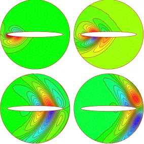
Figure 1: Scattered field solution at snapshots in time.
interpolation scheme. Prior to projecting, the solution on the top of previous time-slab, t−n, is interpolated with,
u(x, t−n) =
DXn−1
A=1
NA−(x)uhA(t−n) + ∆xA· ∇u∗A(xcA, t−n)
(15)
where, ∆xA = (x−xA) and the vector, ∇u∗A(xcA, t−n) is the recovered gradients obtained by
superconvergent patch recovery (SPR) at node A, [7] evaluated at the midpoint between node xA, and position x. A similar technique is used for v(x, t−n). This scheme may be viewed as a
correction to standard interpolation, and provides nearly an order-of-magnitude improvement in accuracy. The spatial and temporal error estimates and adaptive strategy we use is similar to that given in [8]; the main improvements are the use of our superconvergent interpolation (projection) technique together with an improved mesh distribution parameter [9].
Numerical Example
Consider scattering of a plane wave at 30o incidence, defined by a Ricker pulse, by a rigid elliptic cylinder. The high-orderp= 6, nonreflecting boundary conditions are applied on a surrounding circle. Figure 1 shows the adaptive solution on linear triangles with spatial, and temporal error tolerances 10% and 0.5% respectively. The corresponding spatial mesh tracking the scattered solution is shown in Figure 2.
Conclusions
Figure 2: Adaptive mesh tracking scattered solution.
Support for this work was provided by the National Science Foundation under Grant CMS-9702082 in conjunction with a Presidential Early Career Award for Scientists and Engineers (PECASE).
References
[1] Thompson, L.L., and Huan, R., “Computation of Far Field Solutions Based on Exact Nonreflect-ing Boundary Conditions for the Time-Dependent Wave Equation”,Computer Methods in Applied Mechanics and Engineering, 190, (2000), 1551-1577.
[2] Thompson, L.L., and Huan, R., “Computation of Transient Radiation in Semi-Infinite Regions Based on Exact Nonreflecting Boundary Conditions and Mixed Time Integration”,Journal of the Acoustical Society of America, 106 (6), pp. 3095-3108, December 1999.
[3] Huan, R., and Thompson, L.L., ‘Accurate Radiation Boundary Conditions for the Time-Dependent Wave Equation on Unbounded Domains’,International Journal for Numerical Methods in Engineer-ing, 47, pp. 1569 - 1603, 2000.
[4] Thompson, L.L., and Huan, R., D. He; “Accurate radiation boundary conditions for the two-dimensional wave equation on unbounded domains”,Computer Methods in Applied Mechanics and Engineering, 191 (2001) 311-351.
[5] Thompson, L.L., and Pinsky, P.M., “A Space-time finite element method for the exterior struc-tural acoustics problem: Time-dependent radiation boundary conditions in two spatial dimensions”, International Journal for Numerical Methods in Engineering,39, pp. 1635-1657, 1996.
[6] Thompson, L.L., “A multi-field space-time finite element method for structural acoustics”, Pro-ceedings of the 1995 Design Engineering Technical Conferences,Acoustics, Vibrations, and Rotating Machines, Vol. 3, Part B, ASME, pp. 49 - 64, Boston, Mass., Sept. 17-21, 1995.
[7] O. C. Zienkiewicz, J. Z. Zhu, ‘The superconvergent patch recovery and a posterior error estimates. Part 1: The Recovery technique‘, International Journal for Numerical Methods in Engineering, Vol.33, 1331-1364, 1992.
[8] Li, X., Wiberg, N.-E., ‘Implementation and adaptivity of a space-time finite element method for structural dynamics‘,Computational Methods in Applied Mechanics and Engineering,156, 211-229, 1998.
[9] P. Coorevits, P. Ladeveze, J.-P. Pelle, ‘An automatic procedure with a control of accuracy for finite element analysis in 2D elasticity‘, Computational Methods in Applied Mechanics and Engineering,