Energy Prices and Competitiveness in Latin
American Emerging Economies
Jorge Torres-Zorrilla1, Jorge B. Guill´en2
1
CENTRUM-Cat´olica, Lima, Peru 2
Universidad ESAN, Lima, Peru
Abstract This paper presents an evaluation of the impact of international oil
prices on the competitiveness of three emergent economies in Latin America. We
use the methodology of input-output tables for: Peru, Chile and Colombia.
Re-cent outstanding macroeconomic performance of these three emergent countries
caused an increase in their demand for energy, which deepened their trade deficit
of oil. The effects of high petroleum prices are divided into (a) the impact on
costs of new energy prices and (b) the impact on competitiveness. The main
conclusion is that energy inputs today constitute the most important cost for
industries in Peru, Chile, and Colombia. We recommend some policies for energy
efficiency that are consistent with the competitiveness of these three emerging
market economies.
Keywords Energy Management, Competitiveness, Efficiency.
JEL ClassificationH00, H20, H30, Q20, Q40.
1. Introduction and Objectives
Our paper follows the green environmentalist approach1 because we are looking
for an efficient energy system that, at the same time, promotes a competitive
industry for our sample of developing countries. However, we stress the necessity
of a reduction of taxes without reducing the optimal social level of pollution2
and, therefore, set up a competitive framework of industries in the emerging
economies.
Decision makers are confronted today with the sustainability issue.
Man-agement decisions will always have impacts on energy efficiency, emissions and
carbon footprints, impacts on ecosystems, and greenhouse gases. Increasingly,
ecological impacts will be the criteria by which decisions will be judged in the
future. This paper seeks to make a contribution to green management in
emerg-ing economies by focusemerg-ing on the need for clean energy efficiency in the comemerg-ing
years.
According to DeCanio and Watkins (1998), investment in energy efficiency
would encourage any project with positive net present value undertaken by a
firm. This idea is in line with Bernanke (1983), Kester (1984), and Dixit and
Pindick (1994).
Our study sheds light on a fair system of taxes by suggesting how oil taxes
cause domestic firms to lose competitiveness. The public finance school proposes
that optimal taxation must consider the inverse-elasticity rule which states that
tax rates should be inversely proportional to their elasticity of demand; goods
for which demand is inelastic (such as gas or oil) should have a high tax rate
since changing their prices does not create much distortion3 (Slemrod, 1990).
1 For a detailed explanation of this approach, see Frohwein and Hansj¨urgens (2005). 2 For instance, the excessive tax on oil in our sample of developing countries was not created for environmental purposes. The emission of gases within our sample countries is lower than that of industrialized economies which contrast with the tax system between these groups of countries.
3
Conversely, the government should set lower tax rates on price-elastic goods since
small price changes may create large distortions in the quantity demanded.
Many critics of the latter point of view argue that Ramsey´s optimal rule of
taxation brings efficiency instead of equity. According to opponents of Ramsey´s
rule, governments may end up imposing a heavy tax on necessities such as food.
In this way, a policymaker who relies on taxing oil will also sacrifice inequality
for efficiency in the management of government income.
Diamond (1975) tried to solve the puzzle of inequality with a modified version
of Ramsey’s rule. He concluded that equity can be introduced into the optimal
commodity tax system by having higher taxes on the goods consumed
predomi-nantly by the rich.
The latter model is very difficult to apply in practice and, specifically, for our
study because oil is used by the rich and the poor. We are not attempting to
study equity, but previous discussion in the literature reveals the impossibility of
following the optimal tax approach.
When the aim is to combat pollution, Pigouvian taxes are very popular.
Fullerton and Wolverton (2005) demonstrated the equivalence between the
Pigou-vian tax and the combination of a presumptive tax and an environmental subsidy
(two-part instrument). However, in the case of car emissions, Fullerton and West
(2000) proved that a Pigouvian tax does not improve welfare to the same
ex-tent as alternative instruments such as uniform taxes on gas, engine size, and
the age of a car. Agostiniet al. (1992) said that a uniform carbon tax was not
optimal, and they argued that environmental policy should be designed taking
into account the specific economic situation and technological choices of each
country4.
We may infer that there is no optimal instrument that can assure reduction of
tax on gas and improved welfare. In our study, we focus attention on the impact
4
of taxes on competitiveness. Authors such as Knoll (2006) have described two
models of competitiveness called the conduit or new money and the investor or
old money models. For Knoll, a neutral tax system does not change the relative
valuation of any investment. In a later analysis, Tannenwald (2004) emphasized
the need to set up a tax system that promotes competitiveness in Massachussets.
We follow the latter idea because oil and energy prices have increased
dra-matically in recent years (IMF, 2008)5. As a result, analysts have observed that
energy is becoming the most important and expensive input for all industries in
emerging economies. The latter situation may affect competitiveness.
The primary objective of the paper is to estimate the present magnitude of
energy inputs for industrial sectors of a group of economies in South America.
To achieve this goal, we use the methodology of input-output tables (Miller and
Blair, 1985) for three emerging economies in Latin America: Peru, Chile and
Colombia. The methodology can receive many critics but there is not a unique
estimation that may capture the effect of oil shock on industry cots or
competi-tiveness.
The increase in the price of oil also implies substantial increases in the price
of all energy sources, including electricity. Some issues limit our input-output
methodology to estimate impacts of international commodity prices, in general,
and oil prices, in particular. Some authors argue that impacts in domestic process
are not linearly related to changes in world commodity prices. Regarding the later
issue, there is an interesting analysis in the literature, for instance, Bernanke,
Gertler and Watson (1997) using a VAR methodology, conclude that the effect of
oil shock prices in the economy comes from a tight of monetary policies instead of
the shock per se. In addition to the later analysis, Hamilton (2003) examines the
nonlinearity between oil price changes and GDP. For him, increasing oil prices
5
affect more than its reduction. He claims that oil price increases disrupt spending
of consumer and firms on certain sectors.
However, for Hamilton and Herrera (2004) the study of Bernanke, Gertler and
Watson (1997) underestimates the effect of oil shock prices in their VAR analysis.
An evidence of the last claim comes from prolonged effect of an oil shock after
three or four quarters. Also, Huntington (2004) finds a significant relationship
between the impacts of an oil shock specifically when the economy is operating
to its full-employment level prior to the disruption.
By the other side, Hunt (2006)6 captures both the supply of, and demand
for, energy in a way to consider many of the major economic channels through
which energy influences the economy. The simulation results suggest that the
acceleration in energy prices alone cannot account for the stagflation experienced
throughout the 1970s.
Like Hamilton (2003), Jimenez-Rodriguez and Sanchez (2005) find a non
lin-ear relationship between inflation and GDP. They also claim that oil importing
countries have negative effect on the economy after a shock in oil prices. In a
theoretical and empirical analysis, Jones, D.W., P.N. Leiby, and I.K. Paik (2004)
show how asymmetric intra and intersectoral reallocations pops up in response
to oil price shocks.
We intend to test the hypothesis that energy has become the most important
input for industries today, especially for emerging economies.
The paper is organized as follows: the next sections evaluate the costs
associ-ated with new energy prices in Peru, Chile and Colombia and provide an analysis
of the impact of those costs on competitiveness. The final section presents some
conclusions and recommendations.
6
2. Impact of New Energy Prices on Costs in Peru, Chile and
Colom-bia
The section presents estimations of the impact of new energy prices, applying the
input-output methodology7. We first evaluate the cost pressures on each country
and then use this as a primary step to calculate the impact of new energy prices
on these economies.
2.1. Cost Pressures in Peru
Unfortunately, the Peruvian input-output matrix was estimated by Instituto
Na-cional de Estad´ıstica e Inform´atica for the base year 1994 (INEI, 2000). Some
economists consider this matrix obsolete, 14 years later, especially because the
oil price averaged only $16 per barrel in world markets in 1994 (IMF, 2008).
On the other hand, we have an updated input-output table for Peru for 2002
(MINCETUR, 2006). The average world price for oil in 2002 reached $25 a barrel
(IMF, 2008), which is still low compared to today standards. Nevertheless, we use
the 2002 input-output matrix to present calculations of the impact of oil price
on costs8.
To initiate the analysis, we follow the input-output model to state that an
estimate of a new level of prices at the sector level is given by the following
formula:
△Pj=△Penergy·(I−A)−1 (1)
7
During 2007 and the first half of 2008, the World has witnessed a spectacular increase of oil prices that precede a significant decrease in the second half of 2008, variations caused by the international financial crisis. However, the real fact is that the funda-mentals of the oil market are that supply is being reduced due to resource depletion. Within the next few years, we will see a constant oil prices increase. The return of $100-a-barrel-prices will be a consequence of the inevitability of oil depletion. The validity of this paper is guaranteed in spite of the actual low prices.
8
where (I−A)−1 is the original inverse input-output matrix,△P
energy is a
row-vector with the increase in the price of energy, and△Pj is a row-vector with the
resultant increase in the prices of all sectors.
To make this model work for the Peruvian case, we assume that the new price
of energy will be reflected on an initial 100%9 increase in the oil price10. Then
we compute the price variable. The sectors that will be most affected by this
increase are given in Table 1.
Table 1: Impact of the oil price: first round.Source: Estimations from input-output table, Peru 2002 (MINCETUR, 2006).
Sector Impact %
Refined petroleum 100
Fishing 8
Transport 8
Iron & steel 5
Non-metals 5
Fishmeal 4
Non-ferrous metals 4
Chemicals 4
Electricity & water 3
Table 1 shows that the sectors most affected are refined petroleum (gas &
diesel) with 100% increase. The impact is also significant for sectors with a high
fuel-component in their costs such as fishing (8%) and transport (8%), iron and
steel (5%), and non-metal industries (5%). Electricity only increased by 3%
be-cause thermal electricity generation was not important in 2002.
However, oil prices have not increased by merely 100% from 2002 to today
(2008). Prices have quadrupled from $25 a barrel to over $100 a barrel in 2008.
9 To make this matrix comparable to today’s prices and also to the matrices of other countries, we have to do some modifications.
10
This increase represents an increase of over 300%. A naive observation would be
that we have to triple the values of Table 1, to go from a 100% effect to a 300%
effect.
Unfortunately, the input-output model assumes constant technical coefficients.
Therefore, the model should only be applied to estimate marginal changes in all
variables. However, increases of 100%, 200%, or 300% of a key input, such as
petroleum, definitely change the technical coefficients. Therefore, impact analysis
of a second 100% increase will require a previous adjustment of all input-output
coefficients, which is far beyond the scope of our study.
What we can do here is to make an assumption for a second-round impact
analysis. Note that this means a re-estimation of the new effects of oil prices,
over and above the values in Table 1.
In this case, we assume that only the fuel coefficients change for every sector
of the input-output matrix, and they approximately double their value. This
means an increase in total costs without changing other coefficients, assuming
that profits (or other items) decrease by the same amount. This new technical
coefficients matrix is used for the second round.
An estimate of a new level of the coefficient of the energy input at the sector
level is given by the following formula:
Aij =aij
Penergy
Pproduct
(2)
Whereaij is the original input-output energy coefficient,Aij is the new
input-output energy coefficient,Penergy is the new price of energy, andPproduct is the
new price of the sectorj being analyzed.
Table 2 provides the impact on prices of a second-round 100% oil price
in-crease, estimated with the adjusted matrix. Note that oil prices grow from 1 to
2 in round one and from 2 to 4 in round two. This is equivalent to the increase
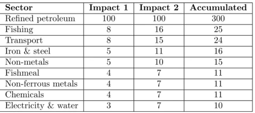
Table 2: Impact of the oil price: second round.Source: Estimations from input-output table, Peru 2002 (MINCETUR, 2006).
Sector Impact 1 Impact 2 Accumulated
Refined petroleum 100 100 300
Fishing 8 16 25
Transport 8 15 24
Iron & steel 5 11 16
Non-metals 5 10 15
Fishmeal 4 7 11
Non-ferrous metals 4 7 11
Chemicals 4 7 11
Electricity & water 3 7 10
In summary, for the second round, we increase coefficients to approximately
double, leaving unchanged all other coefficients; then, we estimate a second
im-pact of 100% increase in oil prices; and finally, we accumulate the two rounds.
The sector affected most is refined petroleum (300%). Then we have fishing
(25%), transport (24%), iron and steel (16%), non-metals (15%), and electricity
(10%). Note that these estimates assume a full impact on domestic fuel prices
and the removal of all subsidies that are still present in the Peruvian domestic
market.
2.2. Magnitude of the Energy Input in Peru
Now we are ready to estimate the present level of energy inputs in the Peruvian
economy. Note that the high oil price also implies substantial increases in the price
of all energy sources, including electricity. The thesis is that energy has become
the most important input for all industries, especially in emerging economies.
We define energy inputs as the sum of fuels + electricity11 (sectors 22 & 32 of
11
the Peruvian input-output matrix). Remember that the new coefficient of energy
inputAij is estimated from the formula:
Aij =aij
Pf uels
Pproduct
(3)
After round two, a second 100% increase in oil price, the magnitude of the energy
input for all sectors is presented in Table 3.
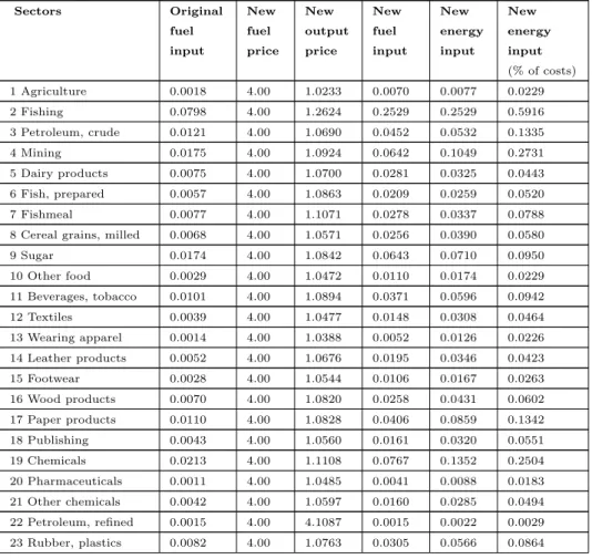
Table 3: (Peru) Magnitude of energy input after 300% increase in oil prices12.
Sectors Original fuel input New fuel price New output price New fuel input New energy input New energy input
(% of costs) 1 Agriculture 0.0018 4.00 1.0233 0.0070 0.0077 0.0229 2 Fishing 0.0798 4.00 1.2624 0.2529 0.2529 0.5916 3 Petroleum, crude 0.0121 4.00 1.0690 0.0452 0.0532 0.1335 4 Mining 0.0175 4.00 1.0924 0.0642 0.1049 0.2731 5 Dairy products 0.0075 4.00 1.0700 0.0281 0.0325 0.0443 6 Fish, prepared 0.0057 4.00 1.0863 0.0209 0.0259 0.0520 7 Fishmeal 0.0077 4.00 1.1071 0.0278 0.0337 0.0788 8 Cereal grains, milled 0.0068 4.00 1.0571 0.0256 0.0390 0.0580
9 Sugar 0.0174 4.00 1.0842 0.0643 0.0710 0.0950
10 Other food 0.0029 4.00 1.0472 0.0110 0.0174 0.0229 11 Beverages, tobacco 0.0101 4.00 1.0894 0.0371 0.0596 0.0942 12 Textiles 0.0039 4.00 1.0477 0.0148 0.0308 0.0464 13 Wearing apparel 0.0014 4.00 1.0388 0.0052 0.0126 0.0226 14 Leather products 0.0052 4.00 1.0676 0.0195 0.0346 0.0423 15 Footwear 0.0028 4.00 1.0544 0.0106 0.0167 0.0263 16 Wood products 0.0070 4.00 1.0820 0.0258 0.0431 0.0602 17 Paper products 0.0110 4.00 1.0828 0.0406 0.0859 0.1342 18 Publishing 0.0043 4.00 1.0560 0.0161 0.0320 0.0551 19 Chemicals 0.0213 4.00 1.1108 0.0767 0.1352 0.2504 20 Pharmaceuticals 0.0011 4.00 1.0485 0.0041 0.0088 0.0183 21 Other chemicals 0.0042 4.00 1.0597 0.0160 0.0285 0.0494 22 Petroleum, refined 0.0015 4.00 4.1087 0.0015 0.0022 0.0029 23 Rubber, plastics 0.0082 4.00 1.0763 0.0305 0.0566 0.0864
12
Table 3: (continuation).
24 Non-metals 0.0301 4.00 1.1487 0.1048 0.1687 0.2769 25 Iron & steel 0.0348 4.00 1.1742 0.1187 0.1596 0.2303 26 Non-ferrous metals 0.0091 4.00 1.1132 0.0327 0.0683 0.0805 27 Metal products 0.0054 4.00 1.0840 0.0201 0.0324 0.0592 28 Machinery n.e.d 0.0119 4.00 1.1010 0.0434 0.0550 0.0853 29 Machinery E. 0.0077 4.00 1.0818 0.0285 0.0445 0.0680 30 Transport equipment 0.0061 4.00 1.0906 0.0222 0.0399 0.0553 31 Other manufactures 0.0059 4.00 1.0708 0.0222 0.0400 0.0683 32 Electricity & water 0.0265 4.00 1.1021 0.0960 0.1175 0.4014 33 Construction 0.0098 4.00 1.0843 0.0361 0.0375 0.0713 34 Commerce 0.0027 4.00 1.0493 0.0102 0.0224 0.0767 35 Transports 0.0688 4.00 1.2488 0.2204 0.2259 0.4139 36 Services, financial 0.0012 4.00 1.0273 0.0046 0.0206 0.0658 37 Insurance 0.0012 4.00 1.0175 0.0047 0.0064 0.0115 38 Rental 0.0000 4.00 1.0055 0.0000 0.0000 0.0000 39 Services, enterprises 0.0035 4.00 1.0303 0.0134 0.0246 0.0702 40 Restaurants, hotels 0.0039 4.00 1.0435 0.0149 0.0234 0.0513 41 Services, households 0.0013 4.00 1.0231 0.0051 0.0110 0.0369 42 Services, households 0.0048 4.00 1.0633 0.0179 0.0277 0.0415 43 Health, private 0.0016 4.00 1.0259 0.0062 0.0199 0.0521 44 Education, private 0.0061 4.00 1.0353 0.0234 0.0373 0.1546 45 Government 0.0096 4.00 1.0489 0.0367 0.0485 0.1677
The first column is the original energy input as a percentage of the gross value
of output of every sector (the original input-output coefficient). The second and
third columns are the price index of fuels and the price indexes of the different
sectors (accumulated for first and second rounds). The fourth column is the
new input-output coefficient after second round. This new coefficient Aij is our
objective and is estimated from the formula above. Note that the oil price index
is now 4.00. That is, in round one, it goes from 1 to 2, and in round two, from 2
to 4.
The final result is that the simple average of the new energy input is 6% for
the goods-producing sectors 1 to 32. Note that this figure is a percentage of gross
value of output (GVO). In order to express this as a percentage of production
VA coefficient is about 50%, the energy input is about 12% of total costs of
production.
Of course, for some sectors, the new energy input reaches a greater level as
a percentage of costs (see seventh column of Table 3). The highest values are
for fishing (59% of costs), transport (41%), electricity (40%), mining (27%),
non-metal products (28%), chemicals (25%), and iron and steel (23%). The final result
is that the simple average of the new energy input is 12% for all goods-producing
sectors.
A conclusion of the above analysis is that energy inputs today constitute the
most important cost for industries in Peru. This may be asserted because the
total sales of energy (sum of the “fuels and electricity” rows from the
input-output matrix) are greater that intermediate sales of other sectors of the matrix.
2.3. Cost Pressures in Chile
The input-output matrix for Chile was estimated by Banco Central de Chile
(2008) for the base year 2003. Remember that oil prices averaged $29 per barrel
in world markets in the year 2003 (IMF, 2008) and that this price was still low
compared to standards of today. We use this 2003 input-output matrix to present
calculations of impact of price increases on costs in Chile.
To initiate the analysis, we use the previously presented formula 1 to estimate
a new level of prices at the sector level.
We apply the model to Chile in two steps as we did in the calculations for
Peru. We assume that the new price of energy will be reflected on an initial
100% increase in the oil price. Then, we compute the price effects. The ranking
of sectors most affected by this increase is given in Table 4.
However, again, as in the Peruvian case, oil prices have not increased by
merely 100% from 2003 to 2008. Prices have more than tripled from $29 a barrel
Table 4: Impact of the oil price: first round.Source: Estimations from input-output table, Chile 2003 (Banco Central de Chile, 2008.
Sector Impact %
Fuels 100
Passenger transport 15
Truncking 13
Rail transport 9
Agriculture 8
Sugar 6
Air transport 6
Fruits 5
Coal 4
Milling 3
As before, a naive observation would be that we have to multiply the values of
Table 1 by 2.5 to go from a 100% effect to a 250% effect.
The input-output model assumes constant technical coefficients, and
there-fore, the model should only be applied to estimate marginal changes in all
vari-ables. An oil price increase of 250% definitely changes the technical coefficients.
Therefore, impact analysis of a second increase will require a previous adjustment
of all input-output coefficients, which is far beyond the scope of this preliminary
study.
What we do here is to make the same assumption as before for a second-round
impact analysis. Note that this means a new estimate of the effect of oil prices,
over and above the values in Table 4. We assume that only the fuel coefficients
change, for every sector of the input-output matrix, and they approximately
double their value. This means an increase in total costs without changing other
coefficients, assuming that profits or other items decrease by the same amount.
This new technical coefficients matrix is used for the second round.
We use the same formula (2) to estimate a new coefficient of the fuel-energy
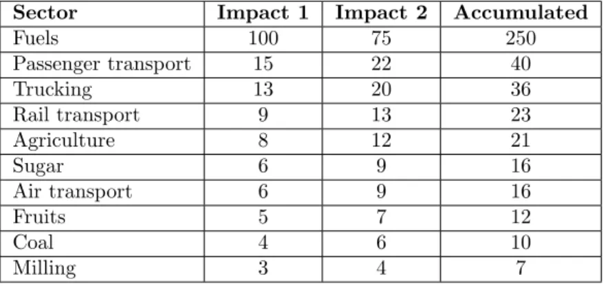
Table 5 provides the impact on prices of a second-round 75% oil price increase.
Note that oil prices increased from 1 to 2 in round one and from 2 to 3.5 in round
two. This is equivalent to the increase from $29 to $102 per barrel13.
Table 5: Impact of oil price: second round.Source: Estimations from input-output table, Chile 2003 (Banco Central de Chile, 2008).
Sector Impact 1 Impact 2 Accumulated
Fuels 100 75 250
Passenger transport 15 22 40
Trucking 13 20 36
Rail transport 9 13 23
Agriculture 8 12 21
Sugar 6 9 16
Air transport 6 9 16
Fruits 5 7 12
Coal 4 6 10
Milling 3 4 7
In summary, for round two, we increase coefficients to approximately double,
leaving unchanged all other coefficients; then, we estimate a second impact of
75% in oil prices; and finally, we accumulate the two rounds.
The sector most affected is again refined petroleum (250%), followed by
pas-senger transport (40%), trucking (36%), rail transport (23%), agriculture (21%),
sugar (16%), and air transport (16%). Electricity only increased by 2% (see Table
5).
2.4. Magnitude of the Energy Input in Chile
Now, we are ready to estimate the present level of energy inputs in the Chilean
economy. Note that, in the case of Chile, the high oil price does not imply
substan-13
tial increases in the price of electricity. Nevertheless, we add fuel and electricity
inputs to estimate total energy inputs.
The new coefficient Aij is again estimated from the formula (3) used before.
After round two, a second increase in oil price, the magnitude of the energy input
for all sectors is presented in Table 6.
Table 6: Chile: Magnitude of energy input after 250% increase in oil prices.
Sectors Original fuel input New fuel price New output price New fuel input New energy input New energy input
Table 6: continuation.
30 Wood products 0.0047 3.50 1.0396 0.0158 0.0350 0.0690 31 Paper products 0.0103 3.50 1.0499 0.0343 0.0576 0.1148 32 Printing 0.0011 3.50 1.0146 0.0038 0.0116 0.0318 33 Fuels 0.002 3.50 3.5200 0.0020 0.0056 0.0341 34 Basic chemicals 0.0082 3.50 1.0309 0.0278 0.0514 0.1552 35 Other chemicals 0.0033 3.50 1.0163 0.0114 0.0156 0.0513 36 Rubber products 0.0038 3.50 1.0160 0.0131 0.0278 0.0824 37 Plastics 0.0023 3.50 1.0145 0.0079 0.0276 0.0806 38 Glass products 0.0277 3.50 1.0770 0.0900 0.1159 0.4240 39 Other non-metal products 0.0233 3.50 1.0810 0.0754 0.0985 0.2303 40 Iron & steel 0.0049 3.50 1.0231 0.0168 0.0587 0.1963 41 Non-ferrous metals 0.0042 3.50 1.0269 0.0143 0.0296 0.0722 42 Metal products 0.0039 3.50 1.0184 0.0134 0.0275 0.0855 43 Non-electric machinery 0.0033 3.50 1.0168 0.0114 0.0243 0.0641 44 Electric machinery 0.0036 3.50 1.0214 0.0123 0.0312 0.0713 45 Transport equipment 0.0035 3.50 1.0145 0.0121 0.0182 0.0650 46 Furnitures 0.0026 3.50 1.0206 0.0089 0.0205 0.0472 47 Other manufacturing 0.0023 3.50 1.0139 0.0079 0.0182 0.0542 48 Electricity 0.0102 3.50 1.0420 0.0343 0.3573 0.7821
49 Gas 0.0718 3.50 1.1922 0.2108 0.2207 0.4345
Table 6: continuation.
70 Public health 0.0023 3.50 1.0111 0.0080 0.0131 0.0671 71 Private health 0.0008 3.50 1.0053 0.0028 0.0064 0.0423 72 Entertainment activities 0.0014 3.50 1.0163 0.0048 0.0191 0.0508 73 Other services 0.0086 3.50 1.0327 0.0291 0.0370 0.1280
The first column is the original fuel input as a percentage of gross value of
output of every sector (the original input-output coefficient). The second and
third columns are the price index of fuels and the price indexes of the different
sectors (accumulated for first and second rounds). The fourth column is the
new input-output coefficient after second round. This new coefficient Aij is our
objective, and it is estimated from the formula above. Note that the oil price
index is now 3.5. That is, in round one, it increased from 1 to 2 and in round
two, from 2 to 3.5.
The final result is that the simple average of the new energy input is 6% for
all goods-producing sectors 1 to 51 (as a percentage of GVO). To express this as
a percentage of costs, we discount value added from the GVO.
Of course, for some sectors, the new energy input reaches a greater level as
a percentage of costs (see seventh column of Table 6). The higher values are for
passenger transport (93% of costs), truck transport (77%), electricity (78%), rail
transport (50%), air transport (44%), and Gas (44%). The final result is that the
simple average of the new energy input is 13% for all goods-producing sectors 1
to 51.
This result goes along the line of De Miguel, O’Ryan, Pereira and Carriquiri
(2006) who studied in a General Equilibrium Model how oil price increase and the
restrictions to natural gas imports from Argentina affect negatively the Chilean
economy. They analyze quantitatively the direct and indirect effects of these
international shocks. They also claim that policies that promote alternative use of
how their methodology has the problem of ignoring the consumer preferences,
transmission channels that cannot be captured.
As in the Peruvian case, the conclusion of our above analysis is that fuels and
energy inputs today constitute the most important cost for industries in Chile.
That is, the total sales of energy are greater that intermediate sales of other
sectors of the matrix.
2.5. Cost Pressures in Colombia
The input-output matrix for Colombia was estimated by Departamento
Admin-istrativo Nacional de Estad´ısticas for the base year 2006 (DANE, 2008). The oil
price averaged $64 per barrel in world markets in the year 2006 (IMF, 2008).
Al-though this price is less than the standard price as of today, the case is different
from the cases for Peru and Chile. In this case, we do not need to re-estimate
new energy coefficients to refine cost-price estimations, and we directly use the
2006 input-output matrix to make calculations.
To initiate the analysis, we use the previously presented formula (1) to
esti-mate a new level of prices at the sector level.
As observed, we apply the model to Colombia in one step, contrary to the
cases for Peru and Chile14. We assume that the new price of energy will be based
on a final 60% increase of the oil price. Then, we compute the price effects. The
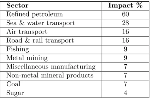
ranking of sectors most affected by this increase is given in Table 7.
The sectors for which the impact is greatest would be fuels with a 60%
in-crease and other sectors with a high fuel-component in their costs. These are sea
transport (28%), air transport (16%), and road and rail transport (16%). The
impact is also significant for fishing (9%), metal mining (9%), non-metal
min-eral products (7%), coal (7%), and sugar (4%). Note that electricity increases by
14
Table 7: Impact of oil price.Source: Estimations from input-output table, Colom-bia 2006 (DANE, 2008).
Sector Impact %
Refined petroleum 60
Sea & water transport 28
Air transport 16
Road & rail transport 16
Fishing 9
Metal mining 9
Miscellaneous manufacturing 7 Non-metal mineral products 7
Coal 7
Sugar 4
less than 1%; this reflects the fact that thermal generation is not important in
Colombia.
Remember that the input-output model assumes constant technical
coeffi-cients, and therefore, the model should only be applied to estimate marginal
changes in all variables. However, the oil price increased 60%, and this is not
a marginal change. Nonetheless, we assume that changes in the technical
co-efficients are not as high as that, and we do not make an adjustment of the
input-output coefficients.
2.6. Magnitude of the Energy Input in Colombia
Now, we are ready to estimate the present level of energy inputs in the Colombian
economy. In this case, we also add fuel and electricity inputs to estimate total
energy inputs.
The new coefficient Aij is again estimated from the formula (3) presented
previously. The magnitude of the energy input for all sectors is presented in
Table 8: Colombia: Magnitude of energy input after 60% increase in oil prices. Sectors Original fuel input New fuel price New output price New fuel input New energy input New energy input (% of costs)
1 Coffee 0.0044 1.6 1.0101 0.0070 0.0087 0.0431
2 Other agricultural products 0.0098 1.6 1.0160 0.0154 0.0172 0.0565 3 Live animals & products 0.0088 1.6 1.0130 0.0139 0.0167 0.0565 4 Forestry products 0.0065 1.6 1.0212 0.0102 0.0177 0.0742
5 Fishing 0.1051 1.6 1.0760 0.1563 0.1630 0.5402
6 Coal 0.0808 1.6 1.0649 0.1214 0.1300 0.3018
7 Crude petroleum & Gas 0.0000 1.6 1.0091 0.0000 0.0017 0.0085 8 Metal mining 0.1098 1.6 1.0761 0.1633 0.1926 0.6168 9 Non-metal mining 0.0249 1.6 1.0195 0.0390 0.0472 0.3079 10 Meat & fish 0.0042 1.6 1.0188 0.0066 0.0127 0.0159 11 Vegetable oils 0.0201 1.6 1.0353 0.0311 0.0417 0.0523 12 Dairy products 0.0036 1.6 1.0187 0.0056 0.0165 0.0214 13 Grain milling 0.0088 1.6 1.0232 0.0137 0.0221 0.0300 14 Coffee products 0.0062 1.6 1.0161 0.0098 0.0133 0.0145
15 Sugar 0.0369 1.6 1.0429 0.0566 0.0611 0.0823
Table 8: continuation.
37 Waste 0.0256 1.6 1.0165 0.0402 0.0418 0.9533
38 Electricity 0.0009 1.6 1.0075 0.0014 0.3384 0.6426 39 Gas, homes 0.0300 1.6 1.0291 0.0466 0.0537 0.0848
40 Water 0.0044 1.6 1.0080 0.0069 0.0290 0.1018
41 Construction works, buildings 0.0008 1.6 1.0239 0.0013 0.0013 0.0025 42 Construction works, roads & other 0.0045 1.6 1.0258 0.0070 0.0070 0.0125
43 Trade 0.0057 1.6 1.0160 0.0090 0.0239 0.0712
44 Repare services:automobiles & other 0.0040 1.6 1.0192 0.0062 0.0201 0.0351 45 Hotels & restaurants 0.0043 1.6 1.0175 0.0067 0.0127 0.0220 46 Road & rail transport 0.1988 1.6 1.1321 0.2809 0.2818 0.5534 47 Sea transport 0.4302 1.6 1.2732 0.5406 0.5445 0.8013 48 Air transport 0.2137 1.6 1.1463 0.2983 0.2993 0.4618 49 Services complementary to transport 0.0288 1.6 1.0316 0.0447 0.0671 0.1070 50 Mail & communications 0.0379 1.6 1.0342 0.0587 0.0778 0.1494 51 Financial services 0.0002 1.6 1.0099 0.0003 0.0155 0.0363 52 Real estate services 0.0000 1.6 1.0020 0.0000 0.0001 0.0007 53 Services to firms 0.0067 1.6 1.0134 0.0106 0.0225 0.0676 54 Public administration 0.0123 1.6 1.0156 0.0194 0.0244 0.0646 55 Education services 0.0025 1.6 1.0056 0.0039 0.0104 0.0764 56 Social & health services 0.0166 1.6 1.0260 0.0260 0.0472 0.0916 57 Drainage services 0.0163 1.6 1.0178 0.0256 0.0342 0.0860 58 Entertainment services 0.0058 1.6 1.0110 0.0091 0.0270 0.0607 59 Domestic services 0.0000 1.6 1.0000 0.0000 0.0000 0.0000
The final result is that the simple average of the new energy input is only 5%
for all goods-producing sectors 1 to 36. Note that this is a percentage of GVO.
In order to express this as a percentage of production costs, we must discount
value added (VA) from the GVO. Since the average VA coefficient equals 50%,
the energy input is about 10% of total costs of production.
Of course, for some sectors, the new energy input reaches a greater level as
a percentage of costs (see eight column of Table 8). The higher values are for
sea transport (80% of costs), road-rail transport (55%), air transport (46%),
electricity (64%), metal mining (61%), and fishing (54%). The final result is that
the simple average of the new energy input is 10% for all goods-producing sectors
A conclusion of the above analysis is that fuels and energy inputs today
constitute the most important cost for industries in Colombia. That is, the total
sales of energy are greater that intermediate sales of other sectors of the
input-output matrix.
3. Impact on Competitiveness (Costs)
The effects on costs of high petroleum prices on new energy prices were presented
in the previous section. The impact of these effects on the competitiveness of the
three countries of our sample is discussed here.
First, we have to mention that regarding substitution effects, we explicitly
made the assumption that there are no direct substitutes for energy in the
indus-tries of the surveyed emerging economies, in the medium term. That is to say,
it is not viable to replace other factors instead of energy in response to relative
price changes. In fact, other studies demonstrate that the elasticity of
substitu-tion between energy and other inputs is low and close to zero in most industries
of emerging economies as today. A World Bank study reports that an estimate of
the elasticity of substitution between energy and other inputs equals about 0.25
for a three region model of energy international trade (Martin R. and Selowsky
M., 1981)
Solving the problem of the last effect, we have to argue that to be
compet-itive15 in this new age of globalization, whenever energy costs increase and if
energy becomes the most important input in manufacturing industries, we worry
about the net effects on competitiveness. If we already have competitive
tages for a given industrial product, we should worry if our country is likely to
lose that competitive advantage because of the new energy prices.
Second, if energy is the most important input for industries today, we should
try to rely on cheap sources of energy. For this, the least we can do is to consider
removing all taxes on energy inputs, that is, fuels and electricity. This means
that all indirect taxes on fuels must be removed, including general sales taxes
and excise taxes.
This set of countries did not find alternatives to gas because their lack of
high technology in their firms (Wijetilleke, Lakdasa and Suhashini K., 1995).
Consequently, rising oil prices hit harder in emerging economies. These countries
are also dependent on oil imports for fuels and also for electricity generation and
they do not have nuclear power facilities, wind/solar power infrastructure, as
developed countries do. In sum, they will be more affected, in relative terms, in
their competitiveness.
Our result goes along the line of Jimenez-Rodriguez and Sanchez (2005) and
Jones, Leiby and Paik (2004) because the impact of oil prices affects our set of
countries asymmetrically to different sectors. This result is very significant in oil
importing countries.
Bacon (1992), concludes that fuel taxes can reduce air pollution cheaply
through fuel substitution, depending on how flexible activities are with regard
to the fuel used. However, in developing countries there is not much flexibility
because of the low technology.
Table 9 shows how the price of gas in other countries can be so low. In the
USA, the gas price is US$3.45. In addition, as of July 1, 2008, the average amount
of tax imposed on a gallon of gas sold in the United States was 49.4 cents per
gallon (API, 2008). We have estimated the distortion of prices for Peru, Chile
and Colombia. The distortion of prices, expressed in percentage, measures the
distortion is 29%, 69% and 7% in Peru, Chile and Colombia respectively. This
means that the tax system within this sample of countries is very significant.
If all taxes on fuels are removed, we are not against the pro-environment
groups because we try to promote a fair and competitive system for this set of
countries without increasing the social cost of pollution16. There are developed
countries that emit more gases, and they do not have heavy taxes on oil.
Also, many economists (Porter and Claas van der Linde, 1999) argue that
if we look for oil substitutes such as ethanol and biodiesel, this will increase
competitiveness. Additionally, worries about the environment make biofuels an
acceptable alternative of renewable energy. Ethanol is a biofuel that can compete
with oil because of accessible technology and low costs (Porter and Claas van der
Linde, 1999).
Biodiesel and natural gas are another alternative to fossil oil. Natural gas is
very cheap and is used by Europeans (Clementi, 2005). Natural gas does not
contain carbon or any other similar particle; it is renewable17, and therefore, it
is not as harmful to the environment as gas18.
In South America, Venezuela has the largest source of natural gas. Peru has 13
trillion cubic feet–enough to provide the domestic market and exports for decades
(Vargas-Llosa, 2008). The same author says that because the government and
much of the opposition demonized foreign investment, the exploitation of those
reserves began only a few years ago. Therefore, Peru was importing an expensive
resource and making its industry less competitive.
16
Table 10 shows how the per-capita gas emission is high in industrialized countries. Unfortunately, we do not have data for the sample of countries in our study. However, we can infer that their emission of gases would not be comparable to the USA or Western European countries. The 1994 statistics for China are very interesting, and it would be interesting to have up-to-date figures.
17 When it has this characteristic, it is called natural gas which is a biogas obtained from biomass. By upgrading the quality to that of natural gas, it becomes possible to distribute the gas to customers via the existing gas grid and to burn it in existing appliances.
18
The Colombian case is very interesting because there is an impediment to
explode exploiting natural gas. According to Caballero and Reinstein (2004),
policymakers are responsible for the delay in starting the exploitation of natural
gas.
We believe that our study sheds light on the search for alternatives to reduce
the size of companies carbon footprints without losing competitiveness among
the industries in this particular sample of countries.
Table 9: Ranking of cheapest gas in the world19.Source: Associates for Interna-tional Research (AIRINC).
Rank Country Price (US$)/gal
1. Venezuela 0.12
2. Iran 0.40
3. Saudi Arabia 0.45
4. Libya 0.50
5. Swaziland 0.54
6. Qatar 0.73
7. Bahrain 0.81
8. Egypt 0.89
9. Kuwait 0.90
10. Seychelles 0.98
44. United States 3.45
4. Conclusions and Recommendations
The effects of the oil price crisis on emerging economies are multiple. The probable
effects of an oil price of over $100 per barrel include the following: (a) increase
19
Prices in US dollars; 155 countries were surveyed between March 17 and April 1, 2008. Prices are not adjusted for cost of living.
20
Table 10: Gas emission by country20.Source: Carbon Planet.
Country Year CO2e Mt/person
Australia 2000 27.54
USA 2002 24.09
Canada 2003 23.45
Russian Federation 1999 12.91
Netherlands 1999 11.02
United Kingdom 2003 11.01
European Union 1999 10.74
Japan 2002 9.65
Mexico 2000 7.04
Hong Kong 2003 6.39
China 1994 3.05
India 2001 1.34
of oil import value and balance-of-payment deficit, (b) cost pressures over all
economic sectors, (c) recession, and, most importantly, (d) a negative impact on
competitiveness.
We have seen that the impact of the present level of oil prices has been
to increase energy costs to 12%, 13%, and 10% for Peru, Chile and Colombia
respectively. This summarizes the relevance of the energy cost for these countries
today.
Our study goes along the line of Alaimo and Lopez (2008) who find that
OECD countries tend to reduce oil intensity which contrast Latin America
coun-tries (and more generally for middle-income councoun-tries like our sample) where oil
intensities appear to be unaffected by oil prices.
Then, competitiveness is affected negatively within this set of countries when
there is an increase in the price of energy. We recommend restructuring the
existing high oil taxes in these countries in order to make them competitive
Alternative policies should promote the establishment of new power sources
such as solar, eolic, or tidal energy21. These new investments should not alienate
us from our goal of better environmental management and will, at the same time,
allow the countries in the study to be more competitive.
This paper also seeks to make a contribution to green management in
emerg-ing economies by focusemerg-ing on the need for energy efficiency in the comemerg-ing years.
There are many methodologies that can measure the impact of an oil price
in-crease on the economy: Panel Regressions, General Equilibrium Models or Input
Output Matrix. The latter methodologies have some advantages and
disadvan-tages in getting the real impact without ignoring channel transmission, consumer
preferences and producer abilities to change their source of energy.
References
1. Agostini, P., M. Botteon and C. Carraro, (1992): A carbon tax to reduce CO2 emissions in Europe.Energy Economics, 14, 279–290.
2. Alaimo, V. and H. Lopez, (2008): Oil Intensities and oil prices: Evidence for Latin America.World Bank WP.
3. Associates for International Research (AIRINC). Available at : http://money.cnn.com/2008/05/01/news/international/usgas price/index.htm 4. API energy reports, available at: www.api.org
5. Bacon, R., (1992): Measuring the possibilities of interfuel substitution.Policy Re-search WP, 1031, World Bank.
6. Banco Central de Chile (2008),Estad´ısticas Econ´omicas, Tabla Insumo Producto 2003, available at: www.bcentral.cl (accessed 1 September 2008).
7. Bernanke, B. S., (1983): Irreversibility, uncertainty, and cyclical invest-ment.Quarterly Journal of Economics, 97, 85–106.
8. Bernanke, B. S., M. Gertler and M. Watson, (1997): Systematic monetary policy and the effects of oil price shocks.Brookings Papers on Economic Activity, 1, 91– 142.
9. Caballero, C. and D. Reinstein, (2004): Obst´aculos para el desarrollo del gas natural en Colombia, working paper, FEDESARROLLO.
10. C´amara de Comercio de Lima (CCL) Reports.
11. Carbon Planet. Available at http://www.carbonplanet.com/country emissions 12. Clementi, A., (2005): El gas natural, una posibilidad ecol´ogica, available at:
www.swissinfo.org/spa/busca/swissinfo.html?siteSect=881&sid=5752959
13. DeCanio, S. and E. Watkins, (1998): Investment in energy efficiency: do the char-acteristics of firms matter?The Review of Economics and Statistics, 80, 95–107. 14. Departamento Administrativo Nacional de Estad´ısticas (DANE) (2008), Portada
DANE – Colombia, Tabla Insumo Producto 2006, available at: www.dane.gov.co (accessed 1 September 2008).
15. Diamond, P. A., (1975): A many-person Ramsey rule.Journal of Public Economics, 4, 335–342.
16. Dixit, A. K. and R. S. Pindick, (1994):Investment under Uncertainty. Princeton University Press, Princeton, NJ.
17. De Miguel, C., R. O’Ryan, M. Pereira and B. Carriquiri, (2006): Energy shocks, fiscal policy and CO2 emissions in Chile WP. Global Trade an´alisis, Purdue Uni-versity.
18. Frohwein, T. and B. Hansj¨urgens, (2005): Chemicals regulation and the Porter hypothesis: a critical review of the new European chemicals regulation.Journal of Business Chemistry, 2, 19-36.
19. Fullerton, D. and A. Wolverton, (2005): The two-part instrument in a second-best world.Journal of Public Economics, 89, 1961-1975.
20. Fullerton, D. and S. West, (2000): Tax and subsidy combinations for the control of car pollution. Working paper W7774, National Bureau of Economic Research, Cambridge, MA, July 2000.
22. Hamilton, J. D. and A. M. Herrera, (2004): Oil shocks and aggregate macroeconomic behavior: the role of monetary policy.Journal of Money, Credit, and Banking, 36, 265–286.
23. Hunt, B., (2006): Oil price shocks and the U.S. stagflation of the 1970s: some insights from GEM.Energy Journal, 27, 61–80.
24. Huntington, H. G., (2004): Shares, gaps and the economy’s response to oil disrup-tions.Energy Economics, 26, 415–424.
25. International Monetary Fund (IMF), (2008): Estad´ısticas Financieras Interna-cionales. Washington, DC, available at: www.imf.org (accessed 1 September 2008). 26. Instituto Nacional de Estad´ıstica e Inform´atica (INEI), (2000):Tabla Insumo
Pro-ducto de la Econom´ıa Peruana 1994, INEI, Lima, Per´u.
27. Jimenez-Rodriguez, R. and M. Sanchez, (2005): Oil price shocks and Real GDP growth: empirical evidence for some OECD countries.Applied Economics, 37, 201– 228.
28. Jones, D. W., P. N. Leiby and I. K. Paik, (2004): Oil price shocks and the macroe-conomy: what has been learned since 1996.Energy Journal, 25, 1–32
29. Kester, W. C., (1984): Today’s options for tomorrow’s growth.Harvard Business Review, 62, 153–160.
30. Knoll, M., (2006): Taxes and competitiveness. Working paper, University of Penn-sylvania, Philadelphia, PA.
31. Martin R. and M. Selowsky, (1981): An Analysis of Adjustment in Oil-Importing Developing Countries. WP 466.
32. Miller, R. E. and P. D. Blair, (1985):Input-Output Analysis: Foundations and Ex-tensions. Prentice-Hall, Upper Saddle River, NJ.
33. Ministerio de Comercio Exterior y Turismo (MINCETUR) (2006), Desarrollo de una Matriz de Contabilidad Social para el Per´u, Reporte de consultor´ıa no publi-cado, MINCETUR, Lima, Per´u.
34. Organismo Supervisor de la Inversi´on en Energ´ıa y Miner´ıa (OSINERMIN) Reports. 35. Porter, M. and C. Linde, (1995): Toward a New Conception of the Environment
Competitiveness Relationship.Journal of Economic Perspectives, 9, 97-118. 36. Porter, M. and C. Linde, (1999): Green and competitive: ending the stalemate.
37. Slemrod, J., (1990): Optimal taxation and optimal tax systems. Journal of Eco-nomic Perspectives, 4, 157–78
38. Tannenwald, R., (2004): Massachusetts business taxes: Unfair? Inadequate? Un-competitive? Federal Reserve Bank of Boston, Boston, MA.
39. Wijetilleke, L. and K. Suhashini, (1995): Air Quality Mangement: Considerations for Developing Countries.World Bank Technical Paper, 278, Energy Series (Wash-ington DC)