Finding the Number of Groups in Model Based Clustering via Constrained Likelihoods

Finding the Number of Groups in

Model-Based Clustering via Constrained

Likelihoods

Andrea Cerioli

Dipart. di Scienze Economiche e Aziendali, Universit`

a di Parma

Luis Angel Garc´ıa-Escudero

Dpto. de Estad´ıstica e I.O. and IMUVA, Universidad of Valladolid

Agust´ın Mayo-Iscar

Dpto. de Estad´ıstica e I.O. and IMUVA, Universidad of Valladolid

and

Marco Riani

Dipart. di Scienze Economiche e Aziendali, Universit`

a di Parma

June 14, 2016

Abstract

Deciding the number of clusterskis one of the most difficult problems in Cluster Analysis. For this purpose, complexity-penalized likelihood approaches have been introduced in model-based clustering, such as the well known BIC and ICL crite-ria. However, the classification/mixture likelihoods considered in these approaches are unbounded without any constraint on the cluster scatter matrices. Constraints also prevent traditional EM and CEM algorithms from being trapped in (spurious) local maxima. Controlling the maximal ratio between the eigenvalues of the scatter matrices to be smaller than a fixed constant c≥1 is a sensible idea for setting such constraints. A new penalized likelihood criterion which takes into account the higher model complexity that a higher value ofcentails, is proposed. Based on this criterion, a novel and fully automatized procedure, leading to a small ranked list of optimal (k, c) couples is provided. Its performance is assessed both in empirical examples and through a simulation study as a function of cluster overlap.

Keywords: Mixtures, EM algorithm, CEM algorithm, BIC, ICL.

∗_{Research partially supported by the Spanish Ministerio de Econom´ıa y Competitividad and FEDER,}

1

Introduction

Cluster Analysis is the art of clustering a data set intok groups of similar individuals. One

of the main difficulties (and one of the most widely addressed problems) when using Cluster

Analysis methods is how to decide the number of clusters k to be found. Sometimes k is

known in advance because of the application in mind, but most of the timesk is completely

unknown and we want the data set itself to suggest us a “sensible” number of groups.

In this work we tackle the problem from a model-based perspective, where a normality

assumption for the cluster components also holds. We assume that {x1, ..., xn} is the set of

observations in Rp _{to be clustered. Let ϕ(}·_{;µ,Σ) denote the p.d.f. of the p-variate normal}

distribution with meanµand covariance matrix Σ. In model based clustering, there are two

main different approaches depending on whether the mixture or the classification likelihood

function is used.

The first approach is based on maximization of the mixture log-likelihood (MIX) defined

as

Lk(θ) = n ∑

i=1

log

[ _k ∑

j=1

pjϕ(xi;mj, Sj) ]

,

where θ = (p1, ..., pk, m1, ..., mk, S1, ..., Sk) is the set of parameters satisfying pj ≥ 0 and ∑k

j=1pj = 1, mj ∈ Rp and Sj a p.s.d. symmetric p ×p matrix. The optimal set of

parameters based on this likelihood is

b

θMixt,k = arg max

θ Lk(θ). (1)

Once θbMixt,k = (pb1, ...,pbk,mb1, ...,mbk,Sb1, ...,Sbk) is obtained, the observations in the sample

are divided into k clusters by using posterior probabilities. That is, observation xi is

assigned to cluster j if j = arg maxlpblϕ(xi;mbl,Sbl).

The second approach is based on maximization of the classification log-likelihood (CLA)

defined as

CLk(θ) = n ∑

i=1

k ∑

j=1

zij(θ) log (

pjϕ(xi;mj, Sj) )

,

where θ = (p1, ..., pk, m1, ..., mk, S1, ..., Sj) and

zij(θ) =   

1 if j = arg maxlplϕ(xi;ml, Sl)

In this case, the optimal set of parameters is

b

θClas,k = arg max

θ CLk(θ) (2)

and observation xi is now classified into clusterj if zij(bθClas,k) = 1.

Based on the two different likelihood approaches (1) and (2), some proposals exist that

lead to sensible ways for choosing the number of clusters. The basic idea is to maximize on

k some complexity-penalized versions of these two likelihoods. Specifically, it is common

to add complexity penalties terms which take into account the number of free parameters

in the fitted model. Following this idea and taking the usual log-likelihood transformation,

we envisage three different possibilities:

MIX-MIX : kopt = arg min

k {

−2Lk(bθMixt,k) +vk }

MIX-CLA : kopt = arg min

k {

−2CLk(θbMixt,k) +vk }

CLA-CLA : kopt = arg min

k {

−2CLk(θbClas,k) +vk }

wherevk is the penalty term counting the number of free parameters. This term is typically

chosen as

vk= (kp+k−1 +k(p+ 1)p/2) log(n),

if no particular constraints are posed on the scatter matrices S1, ..., Sk. In our notation,

“MIX-MIX” corresponds to the use of the Bayesian Information Criterion (BIC) (see, e.g.,

Fraley and Raftery (2002); Hui et al. (2015)), while “MIX-CLA” corresponds to the use

of the Integrated Complete Likelihood (ICL) method proposed by Biernacki et al. (2000).

The rationale behind the ICL criterion is that “mixture modeling” is a different problem

from “clustering” and, thus, the number of groups obtained as a solution to these problems

may not be the same. “CLA-CLA” is instead rooted in the crisp clustering framework

of (2) and, to our knowledge, is new to this paper. The consideration of weights pj in

classification likelihoods, as done in CLk(θ), goes back to Symons (1981). Bryant (1991)

already mentioned the possible interest in classification likelihoods with weights to choose

the number of groups in clustering, but without adding an extra penalty term for model

The outline of our work is as follows. The need of constraints in model-based clustering

is reviewed in Section 2. Our selected approach is based on the fulfillment of a maximal ratio

constraint for all the eigenvalues of the cluster scatter matrices, i.e. it forces this ratio to be

smaller than a given constant c. Section 3 shows how well-known criteria can be adapted

in this constrained setting in such a way that a “sensible” number of clusters/components

can be found when the constant c is fixed in advance. Section 4 addresses the important

problem of choosing simultaneously both k and c. Furthermore, Section 5 presents an

automatized procedure that returns a ranked small list of “optimal” cluster partitions.

This procedure is illustrated in practice with both simulated and well-known real data

sets. Section 6 describes a simulation study that shows the effectiveness of the proposed

methodology under general settings. Finally, Section 7 concludes and provides some open

lines for future research.

2

Constrained clustering approaches

The need of constraints on the scatter matrices arises because both (1) and (2) are

un-bounded (just take µ1 =x1 and |Σ1| →0). Therefore, the associated maximization turns

out into a mathematically ill-posed problem (see, e.g., Day (1969)). Additionally, the lack

of appropriate constraints often leads the algorithms proposed for numerical maximization

of (1) and (2) to be trapped in local maxima of the likelihood, associated to the detection

of non-interesting “spurious solutions” (see, e.g., McLachlan and Peel (2000)).

The lack of boundedness of (1) and (2) is often circumvented by resorting to

“appro-priate” initializations of the EM or CEM algorithms commonly adopted to maximize them

numerically. Although this strategy is appealing, we note that, in this case, we would not

be exactly trying to maximize the target functions in (1) and (2). In fact, it is known (see,

e.g., Maitra (2009)) that the result of applying EM and CEM algorithms is strongly

de-pendent on the chosen initialization, which may severely affect the value of the associated

likelihoods and, consequently, the choice ofk provided by MIX-MIX, MIX-CLA and

CLA-CLA. For instance, we may have troubles with elongated parallel clusters when using the

k-means method, or we can be affected by undesired “chaining effects” when considering

Furthermore, it is important to note that Cluster Analysis is also not a well-defined

problem from an applied viewpoint. There is nowadays wide consensus about the fact

that clustering techniques should always depend on the final data-analysis purpose, so

that different goals would require the use of different clustering approaches. Along this

line, Figure 1 in Hennig and Liao (2013) shows a toy example – to which we will go

back in Section 5.3 – with a data set obtained as a realization of a mixture of three

well-separated bivariate normal components. Any clustering approach purely based on mixture

modeling would determine the existence of three clusters. However, a “social stratification”

framework, such as that exemplified in Hennig and Liao (2013), would clearly require the

determination of more than three clusters. Similar conclusions could also hold in other

important application fields, such as marketing research, where the construction of relevant

clusters must often be coupled with subject matter aims. We thus argue that clustering

should not be seen as a fully automatic task providing just one single solution and that the

user always has to play an active role in it. The consideration of appropriate constraints

on θ, when maximizing (1) and (2), may allow the user to specify somehow the type of

partitions he/she is actually interested in. This is another major reason that motivates our

interest in introducing constraints in Cluster Analysis.

Some of the available solutions are based on imposing constraints on the elements of

the decomposition of the scatter matrices in the form Sj = λjDjAjDj′, where λj is the

largest eigenvalue of Sj, Dj is the matrix of eigenvectors ofSj and Aj is a diagonal matrix

depending on the eigenvalues of Sj (see, e.g., Banfield and Raftery (1993) and Celeux and

Govaert (1995)). Considering the λj’s, Dj’s and Aj’s as independent sets of parameters,

the idea is to constrain them to be the same among the different j’s or to allow them to

vary in a specified way. The resulting parameterizations can be easily addressed with the

criteria described in Section 1 just by taking into account the number of free parameters.

Another possibility, going back to Hathaway (1985), has been proposed and explored in

Ingrassia and Rocci (2007) and Garc´ıa-Escudero et al. (2008, 2015). The approach is based

This implies maximizing the likelihoods (1) and (2), but imposing that θ∈Θc with

Θc = {

p1, ..., pk with k ∑

j=1

pj = 1;m1, ..., mk in Rp;S1, ..., Sk p.s.d. matrices

with λl(Sj)≤cλq(Sh) for every j, l, h, q }

.

In the above, {λl(S)} p

l=1 stands for the set of eigenvalues for the scatter matrix S. Note

that through the constant c ≥ 1 we are simultaneously controlling discrepancies from

sphericity and differences among cluster scatters. Parameter c can be interpreted as the

square root of the maximal ratio among the lengths of the equidensity ellipsoids defined

by the ϕ(·;mj, Sj) normal densities. Accordingly, we can define two constrained maximum

likelihood problems: the constrained mixture likelihood maximization (MIXc)

b

θc_Mixt,k = arg max

θ∈Θc

Lk(θ), (3)

and the constrained classification likelihood maximization (CLAc)

b

θ_Clasc _,k = arg max

θ∈Θc

CLk(θ). (4)

The algorithms in Fritz et al. (2013) and in Garc´ıa-Escudero et al. (2014) can be used

to approximately solve these constrained maximizations, respectively. In these algorithms

an eigenvalue truncation procedure is applied to enforce the eigenvalues ratio constraint in

the EM and CEM steps.

3

A penalized likelihood approach to choose

k

in

con-strained clustering

We now define the MIXc-MIX, MIXc-CLA and CLAc-CLA criteria for choosing the number

of clusters when following the constrained maximization targets (3) and (4) for a fixed

constant c≥1. This requires a modification of the “penalty term”, which should take into

account the higher model complexity that a higher cvalue entails.

We propose the use of a penalty term vc

k defined as

v_kc =

   

kp+k−1 +k

p(p−1) 2

| {z }

rotation par.

+ (kp−1)

(

1− 1

c

)

+ 1

| {z }

eigenvalue par.

   

We have distinguished, in the scatter matrices, the parameters related to orthogonal

ro-tations – which are not affected by constraints – and those related to the eigenvalues. In

the most constrained case (c = 1), we have that all the eigenvalues are equal, i.e. there

is only one free extra parameter related to the eigenvalues. On the other hand, we

re-cover kp(p+ 1)/2 free parameters for the scatter matrices when we approximate the fully

unconstrained case c→ ∞.

A justification explaining why we consider this “soft” transition between the two

ex-treme cases is as follows. If no constraints are posed on the whole set of eigenvalues of

the scatter matrices, say λ1, ..., λD (with D = k × p), then we have the reference set

A = {(λ1, ..., λD) : 0 ≤ λl}. On the other hand, in the constrained case, we consider the

set B ={(λ1, ..., λD) : 0≤λl≤ cλq for every l ̸=q}. A very simple idea is to consider the

relative volume of set B with respect to A as a complexity measure. Of course, this ratio

between volumes is not well-defined since neither A nor B are bounded sets. However, we

can take into account that

A=∪

t≥0

At and B = ∪

t≥0

Bt,

with At and Bt being sets defined as in the statement of Theorem 3.1.

Theorem 3.1 Let At = {(λ1, ..., λD) : 0 ≤ λl ≤ t} and Bt = {(λ1, ..., λD) : 0 ≤ λl ≤ t; λl≤cλq for every l̸=q}. Then, we have that

Vol(Bt)

Vol(At)

=

(

1− 1

c

)D−1

. (6)

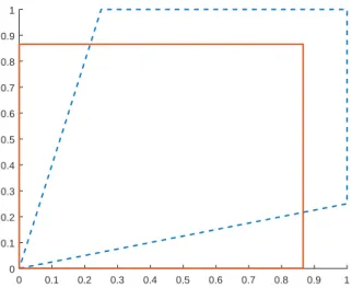
The proof of this technical result is left to the Appendix. Figure 1 shows a graphical

interpretation when t = 1, D = 2 (such as in the case of one group of two-dimensional

observations) andc= 4. In this case Vol(At) = 1 and the ratio Vol(Bt)/Vol(At) equals the

area of a square of side [0,√1−1/c].

Theorem 3.1 is implicitly applied in our definition of the penalty term (5) by seeing that

we have one “principal” eigenvalue and each of the remaining D−1 =kp−1 eigenvalues

are “relatively” weighted by a (1− 1

c) multiplicative factor. By considering the modified

penalty termvc

0 0.1 0.2 0.3 0.4 0.5 0.6 0.7 0.8 0.9 1 0

0.1 0.2 0.3 0.4 0.5 0.6 0.7 0.8 0.9 1

Figure 1: Illustration of Theorem 3.1 when t= 1, D = 2 and c= 4. The surface enclosed

within dashed lines corresponds toB1. Since Vol(A1) = 1, the ratio Vol(B1)/Vol(A1) equals

the area of the square [0,√1−1/4]×[0,√1−1/4] shown with solid lines.

depending on the maximal eigenvalue ratio c:

MIXc-MIX :kopt,MM(c) = arg min

k {

−2Lk(θbMixt,kc ) +v

c k

}

:= arg min

k FMM(k, c)

MIXc-CLA :kopt,MC(c) = arg min

k {

−2CLk(θbcMixt,k) +v

c k

}

:= arg min

k FMC(k, c)

CLAc-CLA :kopt,CC(c) = arg min

k {

−2CLk(θbcClas,k) +v

c k

}

:= arg min

k FCC(k, c).

Differently from the standard MIX-MIX, MIX-CLA and CLA-CLA criteria, the use of

our constrained proposals provides well-defined problems where the corresponding target

functions Fm(k, c), wherem =MM, MC or CC, are bounded. Moreover, spurious solutions

are avoided provided that the supplied value cis not very large; see, Garc´ıa-Escudero et al.

(2015).

The specification of c may be seen as a sensible way for the user in order to play an

active role by declaring the maximum allowed difference on cluster scatters that he/she is

willing to admit. This choice then depends on the final clustering purpose in mind. For

user to specify a value of c close to 1. Choosing c close to 1 implies the search of almost

spherical clusters with similar scatters or, analogously, the use of the Euclidean distance for

clustering. Other problems would require larger values of c which means the detection of

less restricted clusters. Once the value of chas been fixed, the determination of kopt,m(c) is

done by minimizing the previously introduced criteria with respect tok for a given method

m wherem =MM, MC or CC.

It should also be noted that this approach is not affine equivariant due to the lack

of equivariance of the chosen constraints. Therefore, standardizing the variables may be

needed if, for instance, very different scales are involved.

To illustrate how the methodology can be applied, let us consider a simulated data

set of size n = 100 and dimension p = 2 from a k = 3 components mixture obtained by

applying the MixSim method of Maitra and Melnykov (2010), as extended by Riani et al.

(2015) and incorporated into theFSDAtoolbox of Matlab (Riani et al., 2012). The data set

has been generated by imposing an average cluster overlap equal to 0.04 and a maximum

eigenvalue ratio for the scatters matrices equal to 5. Figure 2 shows two scatter plots of

this simulated data set, without and with the “true” assignments labels. It is not perfectly

clear by visual inspection, at least looking at the graph in the left panel, whether there are

two or three clusters.

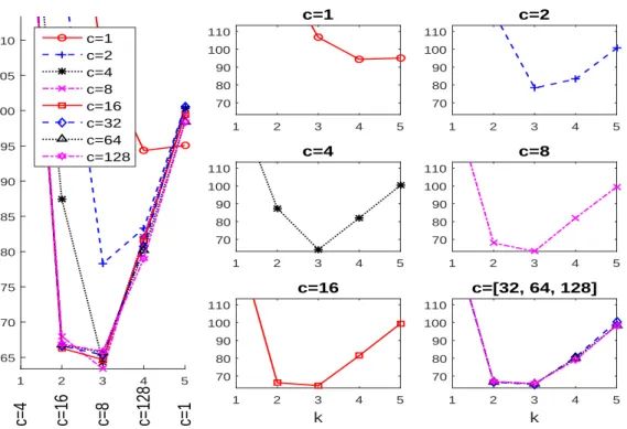
Figure 3 shows the curves of our objective function that are obtained by monitoring

FCC(k, c) (i.e., under the CLAc-CLA criterion), when c ranges in the interval [1,128] and

k goes from 1 to 5. The large left panel shows all the 8 trajectories of FCC(k, c) that

are obtained by considering c = {20,21,22, ...,27}. In this panel, the value of c for the

lowest curve at each k is labeled vertically below the x axis. For instance, when k = 2

the lowest value is for c = 16; for k = 3 the lowest value is for c = 8; etc.. Given that

the eight trajectories strongly overlap, in the first five right panels of this figure we show

what happens for the five smallest values of c we have considered (c = 1,2,4,8,16). The

trajectories for the 3 largest values of c are very similar and, thus, they are all reported in

the same final right panel.

By using the curves plotted in Figure 3, we can see that the optimal values for the

0 0.2 0.4 0.6 0.8 1 1.2 -0.5

0 0.5 1

0 0.2 0.4 0.6 0.8 1 1.2 -0.5

0 0.5 1

Group 2 Group 1 Group 3

Figure 2: Simulated bivariate data set. The panel on the right shows the data set with the

“true” labels and tolerance ellipsoids summarizing the three normal components.

(i.e., when c = 16). We thus obtain k = 3, which corresponds to the true number of

components, when we are interested in neither very spherical nor homoscedastic clusters,

but we find k = 2 clusters when we allow for more elongated group structures. The latter

also provides a sensible cluster partition from a clustering point of view, since only Group

3 seems to be separated from the other populations.

Similar plots are given in Figure 4 whenFMM(k, c) is monitored. We can see that the use

of an objective function more focused on “mixture modeling”, such as MIXc-MIX, always

suggests kopt,MM(c) = 3 (i.e., the true number of mixture components) for every value of

c >1 tried. A higher number of groups is only needed in the case c= 1, due to the strong

assumption of homoscedasticity.

4

Simultaneous choice of

k

and

c

in constrained

clus-tering

Alternatively, we may know the number of groups k due to any economical, physical or

1 2 3 4 5 75 80 85 90 95 100 105 110 115 120

c=4 c=16 c=8 c=64 c=128 c=1 c=2 c=4 c=8 c=16 c=32 c=64 c=128

1 2 3 4 5 80

100 120

c=1

1 2 3 4 5 80

100 120

c=2

1 2 3 4 5 80

100 120

c=4

1 2 3 4 5 80

100 120

c=8

1 2 3 4 5

k

80 100 120

c=16

1 2 3 4 5

k

80 100 120

c=[32, 64, 128]

Figure 3: Analysis of the modified constained criteria when using the CLAc-CLA approach

for the data set shown in Figure 2. The optimal c for each k is shown in the left panel

below the x axis.

this case the user does not want to impose any particular structure to the clusters to be

detected. This goal can be achieved by using the same penalized criteria as before, but

now minimizing on c. Therefore, if k is assumed to be known, we take

copt,m(k) = arg min

c Fm(k, c), for m= MM, MC and CC,

as our choice for the optimal value of c. This information is included in the left panels of

Figure 3 and Figure 4 for the CLAc-CLA and MIXc-MIX criteria, respectively, below the

tick-marks for k on the horizontal axis.

In practice the surely most interesting case is when both the proper number of clustersk

and the constraining factorcare unknown. We have argued before that a fully unsupervised

choice of both parameters, only depending on the data set at hand, is very likely to be out

of reach for most applications. Nevertheless, it would be helpful if we were able to reduce

the space of all the possible choices of the (k, c) parameter pairs to a small list of “sensible”

1 2 3 4 5 65 70 75 80 85 90 95 100 105 110

c=4 c=16 c=8 c=128 c=1 c=1 c=2 c=4 c=8 c=16 c=32 c=64 c=128

1 2 3 4 5 70 80 90 100 110 c=1

1 2 3 4 5 70 80 90 100 110 c=2

1 2 3 4 5 70 80 90 100 110 c=4

1 2 3 4 5 70 80 90 100 110 c=8

1 2 3 4 5

k 70 80 90 100 110 c=16

1 2 3 4 5

k 70 80 90 100 110

c=[32, 64, 128]

Figure 4: Analysis of the constrained criteria when using MIXc-MIX for the data set in

Figure 2. The optimal cfor each k is shown in the left panel below the x axis.

One could think that direct study of the functionals (k, c) 7→ Fm(k, c), for m =

MM, MC and CC, could provide valuable information about how to choose

simultane-ously k and c. With this idea in mind, Figure 5 shows the associated contour plots that

summarize the resulting monitoring process for our three constrained clustering criteria.

Unfortunately, our experience is that these contour plots are not easily interpreted.

Additionally, there are partitions obtained with different (k, c) parameters that correspond

to essentially the same substantial groups, or that simply differ because of the inclusion of

extra (non-interesting) spurious clusters.

5

An automatized procedure for selecting a reduced

list of “sensible” solutions

In this section, we offer a fully automatized procedure that leads to a small and ranked

MIXMIX 75.4138 75.4138 87.3841 87.3841 87.3841 99.3545 99.3545 99.3545 111.3248 123.2952 135.2655 147.2359

20 21 22 23

Restriction factor c

1 2 3 4 5

Number of groups k

MIXCLA 84.2323 84.2323 95.3208 95.3208 106.4093 106.4093 106.4093 117.4978 117.4978 117.4978 128.5863 128.5863 139.6748 150.7633 161.8518

20 21 22 23

Restriction factor c

1 2 3 4 5 CLACLA 83.7358 83.7358 94.8739 94.8739 106.0121 106.0121 106.0121 117.1502 117.1502 117.1502 128.2884 139.4265 150.5647 161.7028

20 21 22 23

Restriction factor c

1 2 3 4 5

Figure 5: Contour plots for the (k, c)7→Fm(k, c) functions when them= MM, MC and CC

criteria are applied.

constrained clustering criteria, relies on analysis of the stability of the cluster partitions

through the Adjusted Rand Index (ARI). Specifically, the procedure first detects a list

with L “plausible” partitions. Such “plausible” partitions may include among them some

partitions that are essentially the same as others already detected, because spurious clusters

made up with few almost collinear or very concentrated data points are found. In a second

step, the partitions including spurious clusters are discarded and we end up with a (typically

very) reduced and ranked list with T “optimal” partitions.

Given a pair (k, c), let P(k, c) denote the partition into k subsets of the n observations

{x1, x2, ..., xn} which is obtained by solving the problem (3) or (4), with the givenk and c

and one of the suggested methods m = MM, MC and CC. Let dARI(A,B) denote the ARI

between partitionsA and B. We consider that two partitions A and Bare “essentially the

same” when dARI(A,B)≥ε, for a fixed threshold ε. Clearly, the higher is the value of the

threshold the greater is the number of tentative different solutions which are considered.

Let us consider the sequencek = 1, ..., K, where K is the maximal number of clusters,

and a sequence c = c1, ..., cC of C possible constraint values. For instance, the sequence

consider a sharp grid of values close to 1. By using this notation, the proposed automatized

procedure may be described as follows:

1. Obtain the list of “plausible” solutions:

1.1 Initialize: Start withK×Cpossible (k, c) pairs to be explored. LetE0 ={(k, c) :

k = 1, ..., K and c=c1, ..., cC}.

1.2 Iterate: Denote byEl−1 the set of pairs (k, c) not already explored at stagel−1.

Then:

1.2.1 Obtain (kl

∗, cl∗) = arg min(k,c)∈El−1Fm(k, c).

1.2.2 Remove all of the cluster partitions (k, c)∈ El−1 withk =k_∗l and values of c

which are adjacent to cl_∗, and such that they are very “similar” to partition

P(kl

∗, cl∗) for the given threshold value ε, in the sense that

dARI(P(k, c),P(kl_∗, cl_∗))≥ε.

Take El as the set El−1 after removing these (k, c) pairs yielding “similar”

partitions.

1.3 Finalize: The iterative procedure ends when EL = ∅ (or when L is a positive

prefixed integer number) and it returns {(k1

∗, c1∗),(k2∗, c∗2), ...,(k∗L, cL∗)} as a list with L “feasible” parameters combinations.

2. Obtain the list of “optimal” solutions:

2.1 Initialize: Start from theL×L matrix (dr,s)r,s=1,...,L, where

dr,s =dARI(P(kr_∗, c_∗r),P(k_∗s, cs_∗)),

and fromI0 ={1, ..., L}.

2.2 Iterate: GivenIt−1 being the non discarded “plausible” solutions at staget−1:

2.2.1 Take (kt

opt, ctopt) = (kl∗t, c∗lt) where lt is the t-th element of It−1 (where the

2.2.2 Discard “spurious” solutions (i.e., those that are similar to the already

de-tected “optimal” ones):

It=It−1\ {r:r ∈ It−1, r > lt and dr,lt ≥ε}.

2.3 Finalize: The iterative procedure ends whenIT =∅and it returns{(kopt1 , c1opt),(k2opt,

c2

opt), ...,(kTopt, cTopt)} as the “optimal” pairs of parameters.

To simplify our notation, we have deleted the subscript m for the criteria used (i.e.,

(k_optt , ct_opt) should be (k_optt _,m, ct_opt,m) for m= MM, MC and CC). Additionally, the complete

automatized procedure is hereinafter referred to autMIXMIX, autMIXCLA and

autCLA-CLA.

For each “optimal” pair (k_optt , ct_opt), it is also informative to take into account the

so-called “best interval” Bt defined as

Bt ={c:Fm(koptt , c

t

opt)≤Fm(ktopt, c)}, (7)

and the so-called “stable interval” defined as

St={c:dARI(P(koptt , c),P(k

t

opt, c

t

opt))≥ε}. (8)

A large interval Bt means that the number of clusterskoptt is “optimal”, in the sense of (7),

for a wide range ofc values. A large intervalSt means that the solution is “stable”, in the

sense of (8), because it does not essentially change when moving c in that interval.

5.1

Application to simulated data

We have applied the proposed automatized procedure with an ARI thresholdε= 0.7 to the

simulated data set displayed in Figure 2. We obtain T = 4 when using the autCLACLA

procedure. The corresponding four best-ranked solutions are shown in Figure 6. We see

that we recover the true number of clustersk2

opt,CC = 3 in the second solution. The solution

with k1

opt,CC = 2 makes perfect sense from the “pure” clustering point of view adopted by

the CLAc-CLA criterion and, thus, it is the first offered partition. The homoscedasticc= 1

solution is shown as the fourth one and it proposes k4

0 0.5 1 1.5 -1

-0.5 0 0.5 1

1.5 Solution 1: k=2 c=16

Best for c=[8-128] Stable for c=[2-128]

0 0.5 1 1.5

-1 -0.5 0 0.5 1

1.5 Solution 2: k=3 c=8

Best for c=[4-128] Stable for c=[1-128]

0 0.5 1 1.5

-1 -0.5 0 0.5 1

1.5 Solution 6: k=5 c=16

Best for c=[4-16] Stable for c=[4-16]

0 0.5 1 1.5

-1 -0.5 0 0.5 1

1.5 Solution 7: k=5 c=1

Best for c=[1-1] Stable for c=[1-1]

Figure 6: The T = 4 best-ranked partitions when using theautCLACLAprocedure for the

simulated data set displayed in Figure 2.

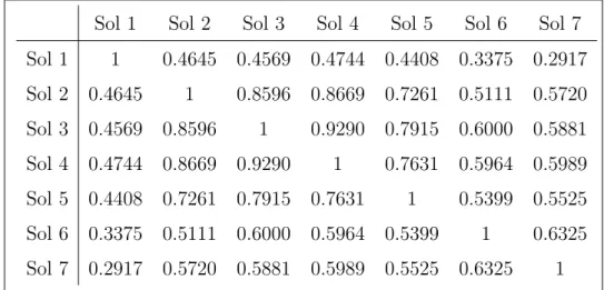
In order to obtain these T = 4 “optimal” solutions, we started from a list (obtained

from Step 1 of the procedure described in Section 5) withL= 7 “plausible” solutions. The

matrix with the ARI distances for this L= 7 partitions (solutions) is shown in Table 1.

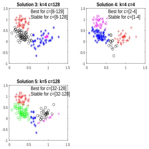
Figure 7 shows theL−T = 3 discarded “spurious” solutions. We can see that these

dis-carded solutions either include clusters made up with few almost collinear or concentrated

observations (solutions 3 and 5), or correspond to solutions close to one already detected

“optimal” partition (solution 4).

Figure 8 shows the ranked set of “optimal” solutions when using the autMIXMIX

procedure. In this case, we find L = 6 and T = 4. Notice that, from a mixture modeling

point of view, we obtain the correct number of components (k_opt1 _,MM = 3) in the first

Table 1: Matrix with the ARI distances for the L= 7 “plausible” solutions

Sol 1 Sol 2 Sol 3 Sol 4 Sol 5 Sol 6 Sol 7

Sol 1 1 0.4645 0.4569 0.4744 0.4408 0.3375 0.2917

Sol 2 0.4645 1 0.8596 0.8669 0.7261 0.5111 0.5720

Sol 3 0.4569 0.8596 1 0.9290 0.7915 0.6000 0.5881

Sol 4 0.4744 0.8669 0.9290 1 0.7631 0.5964 0.5989

Sol 5 0.4408 0.7261 0.7915 0.7631 1 0.5399 0.5525

Sol 6 0.3375 0.5111 0.6000 0.5964 0.5399 1 0.6325

Sol 7 0.2917 0.5720 0.5881 0.5989 0.5525 0.6325 1

suited to address cluster overlap than “pure” clustering, which instead ideally assumes

well-separated clusters.

5.2

Application to the “Iris data set”

The “Iris data set”, originally collected by Anderson (1935) and first analyzed by Fisher

(1936), is considered in this example. We have applied the proposed procedure to this

well-known four-dimensional (p= 4) data set. Figure 9 shows the ranked list of “sensible”

cluster partitions which are automatically found when using the autMIXMIX procedure.

For purposes of clarity we show just the scatter plots of sepal width (SW) vs sepal length

(SL), petal length (PL) vs sepal width (SW) and petal width (PW) vs petal length (PL).

We can see that the most clear two-component partition is the first offered by our

method. In this partition “Iris setosa” is well-separated from “Iris virginica” and “Iris

versicolor” (that are not so easy to separate). The second proposed partition essentially

coincides with the three actual species.

With respect to the third best ranked solution, we recall that this “Iris data set” was

initially collected by Anderson with the aim of seeing whether there was “evidence of

con-tinuing evolution in any group of plants”. Thus, it is interesting to evaluate whether

“vir-ginica” species should be split into two subspecies or not. In their Section 3.11, McLachlan

and Peel (2000) focused only on the 50 virginica iris data and fitted a mixture of k = 2

0 0.5 1 1.5 -1

-0.5 0 0.5 1

1.5 Solution 3: k=4 c=128

Best for c=[8-128] Stable for c=[8-128]

0 0.5 1 1.5

-1 -0.5 0 0.5 1

1.5 Solution 4: k=4 c=4

Best for c=[2-4] Stable for c=[1-4]

0 0.5 1 1.5

-1 -0.5 0 0.5 1

1.5 Solution 5: k=5 c=128

Best for c=[32-128] Stable for c=[32-128]

Figure 7: The L−T = 3 discarded “spurious” solutions detected when using the

autCLA-CLA procedure for the simulated data set displayed in Figure 2.

different quantities summarizing aspects as the separation between clusters, the size of the

smallest cluster and the determinants of the scatter matrices corresponding to these

solu-tions. After analyzing this information, the so-called “S1” solution is chosen as the most

sensible one among the local ML maximizers. It is very nice to see that our third best

ranked solution exactly detects a four-component partition where the “virginica” species

is automatically split into 2 components in such a way that it coincides with the “S1”

partition already proposed in McLachlan and Peel (2000).

5.3

Application to the Hennig and Liao’s type of data

Section 5 in Hennig and Liao (2013) includes a toy example to illustrate that there are

0 0.5 1 1.5 -1

-0.5 0 0.5 1

1.5 Solution 1: k=3 c=8

Best for c=[4-128] Stable for c=[1-128]

0 0.5 1 1.5

-1 -0.5 0 0.5 1

1.5 Solution 2: k=2 c=16

Best for c=[8-128] Stable for c=[4-128]

0 0.5 1 1.5

-1 -0.5 0 0.5 1

1.5 Solution 4: k=5 c=1

Best for c=[1-1] Stable for c=[1-32]

0 0.5 1 1.5

-1 -0.5 0 0.5 1

1.5 Solution 6: k=2 c=2

Best for c=[1-2] Stable for c=[1-2]

Figure 8: The T = 4 “optimal” partitions when using the autMIXMIX procedure for the

data set displayed in Figure 2.

the true clusters” but these clusters “are not necessarily the clusters that a researcher is

interested in”. In the spirit of that toy example, we consider the simulated data set shown

in Figure 10. This data set corresponds to a realization of mixture of three well-separated

bivariate normal components. Without knowledge of the underlying substantial problem,

one would then agree that k = 3 is a sensible choice for k. However, let us assume (as

Hennig and Liao did) that we are facing a social stratification clustering problem and that

the two variables are, for instance, an income and a status indicator. By choosingk = 3 and

very unrestricted scatter matrices, one cluster would contain both the poorest people with

lowest status and the richest people with the highest status. Therefore, in this particular

application, a higher number of (more homoscedastic) clusters is surely needed.

5 6 7 SL 2 3 4 SW

2 3 4

SW 2

4 6

PL

Solution 1: k=2 c=128 Best for c=[128-128] Stable for c=[1-128]

2 4 6

PL 0.5 1 1.5 2 2.5 PW

5 6 7

SL 2

3 4

SW

2 3 4

SW 2

4 6

PL

Solution 2: k=3 c=128 Best for c=[32-128] Stable for c=[16-128]

2 4 6

PL 0.5 1 1.5 2 2.5 PW

5 6 7

SL 2

3 4

SW

2 3 4

SW 2

4 6

PL

Solution 3: k=4 c=128 Best for c=[16-128] Stable for c=[8-128]

2 4 6

PL 0.5 1 1.5 2 2.5 PW

Figure 9: Best-ranked partitions when using autMIXMIX procedure criterion for the “Iris

data set”. Only some few pairs plots are shown for each cluster partition.

using theautMIXMIX procedure. We can see that the best-ranked partition is exactly the

one which discovers the 3 bivariate normal components. On the other hand, the second

and third best ranked partitions offer the user a more sensible clustering partition for

that particular “social stratification” problem. The fourth solution offers a very peculiar

partition where the two more concentrated normal components are surprisingly joined

together. However, this more “exotic” solution just appears after three more “sensible”

ones. In any case, we think that it is useful to reduce all the possible pairs (k, c) to such a

type of small lists of best-ranked partitions, where the user can hopefully choose the one

0 5 10 15 20 0

5 10 15 20

25 Solution 1: k=3 c=32

Best for c=[32-128] Stable for c=[4-128]

0 5 10 15 20

0 5 10 15 20

25 Solution 4: k=5 c=4

Best for c=[4-4] Stable for c=[1-4]

0 5 10 15 20

0 5 10 15 20

25 Solution 5: k=4 c=4

Best for c=[2-4] Stable for c=[1-4]

0 5 10 15 20

0 5 10 15 20

25 Solution 6: k=2 c=64

Best for c=[64-128] Stable for c=[64-128]

Figure 10: Best-ranked partitions when using the autMIXMIX for a data set similar to

that in Hennig and Liao (2013).

6

Simulation study

The purpose of this section is to analyze the performance of theautMIXMIX,autMIXCLA

and autCLACLA procedures as a function of the overlap between the groups.

We have considered an example with clusters with true number of groups equal to 3,

true eigenvalue ratio equal to 6, n = 150, and, an average overlap which goes from 0.01

to 0.1, with step 0.01. We have performed 100 simulations for each setting in dimensions

p = 2 and 6. In each simulation, with the aim of “visiting” as many as possible different

θ vectors, we have considered several random initializations (nstarts=1000) obtained from

drawing k×(p+ 1) observations that are arranged intok groups with p+ 1 observations.

k initial scatter parameters Sj through their sample covariance matrices. In order to start

with an initial admissible solution we have immediately applied the eigenvalue constraint.

The values ofcwhich are considered go from 1 to 128 (c={20,21,22, ...,27}) and the values

of k go from 1 to 5. In order to avoid the randomness due to different starting points, both

for mixture and classification likelihoods, for each simulation we have considered the same

1000 initial subsets for each value of c. For each simulation and each procedure, we have

stored:

1. the ARI between the true solution and the best-ranked solution found automatically;

2. the maximum ARI value between the true solution and the first two best-ranked

solutions found automatically;

3. the maximum ARI value between the true solution and the first three best-ranked

solutions found automatically.

Figure 11 shows the average values of the above ARI over 100 simulations when

dimen-sion of the simulated data set isp= 2. The left panel of the figure shows that as the average

overlap increases the best performance is for the autMIXMIX procedure. More precisely, if

the overlap is small the 3 information criteria give equivalent results, on the other hand as

the overlap increases the gap between autMIXMIX and the other two information criteria

increases. When we consider just the first solution the curve for autMIXCLAand

autCLA-CLA are virtually the same when the average overlap is smaller than 0.04 but the curve

associated withautMIXCLA seems to be slightly higher than that ofautCLACLAfor high

values of overlap. When we consider the first two solutions the curve of autMIXCLA is

always in betweenautMIXMIX andautCLACLA. Finally, when we consider the first three

best solutions the curve of autMIXCLA is virtually equal to that of autMIXMIX even if

autMIXMIX still prevails for large overlap.

In order to show the interest of restrictions, in Figure 11, we have also added the

trajec-tories when we consider MIXc-MIX, MIXc-CLA and CLAc-CLA with a very largec= 1010

value. This extremec almost means that no constraint is imposed on the eigenvalue ratios

of the scatter matrices. Therefore, these curves would essentially correspond to the

0.02

0.04

0.06

0.08

0.10

0.5 0.6

0.7 0.8

0.9 1.0

Best solution

autMIXMIX autMIXCLA autCLA

CLA

MIXMIX 10^10 MIXCLA 10^10 CLA

CLA 10^10

0.02

0.04

0.06

0.08

0.10

0.5 0.6

0.7 0.8

0.9 1.0

Fir

st tw

o solutions

0.02

0.04

0.06

0.08

0.10

0.5 0.6

0.7 0.8

0.9 1.0

Fir

st three solutions

Figure 11: Average ARI index across 100 simulations as a function of the clusters’ overlap

when p= 2. The ARI indexes between the true solution and the best solution are shown

in the left panel; with respect to the first two best-ranked solutions in the central panel

and with respect to first there best-ranked ones in the right panel. The results of

apply-ing “traditional” ICL and BIC criteria (i.e., the use of MIX-MIX and MIX-CLA almost

0.02

0.04

0.06

0.08

0.10

0.2 0.4

0.6 0.8

1.0

Best solution

autMIXMIX autMIXCLA autCLA

CLA

MIXMIX 10^10 MIXCLA 10^10 CLA

CLA 10^10

0.02

0.04

0.06

0.08

0.10

0.2 0.4

0.6 0.8

1.0

Fir

st tw

o solutions

0.02

0.04

0.06

0.08

0.10

0.2 0.4

0.6 0.8

1.0

Fir

st three solutions

Figure 12: Average ARI index across 100 simulations as a function of the clusters’ overlap

when p= 6. The ARI indexes between the true solution and the best solution are shown

in the left panel; with respect to the first two best-ranked solutions in the central panel

and with respect to first there best-ranked ones in the right panel. The results of

apply-ing “traditional” ICL and BIC criteria (i.e., the use of MIX-MIX and MIX-CLA almost

using the MIX-CLA criterium). We can see that the constrained autMIXMIX procedure

clearly outperforms traditional BIC and ICL criteria. Moreover, it appears that gap

be-tween constrained and unconstrained seems to increase as the overlap increases and if we

increase the number of best possible solutions which are kept.

Figure 12 also shows the average values of the above ARI over 100 simulations when

dimension of the simulated data sets is now increased to p = 6. Although this higher

dimensional case yields smaller ARI values than those obtained in the p = 2 case, we

can see that the gap between constrained and unconstrained clearly increases in this new

setting. Note also that very sensible ARI values are obtained, in spite of the higher problem

dimensionality, when retaining the two and three best solutions returned from the proposed

automatized procedures. Finally, we can see that the observed differences associated to

the application of the autMIXMIX, autMIXCLA and autCLACLAprocedures are almost

negligible in this p= 6 case (especially in the central and right panels).

This noticed gap between the proposed methodology and the traditional use of the BIC

and ICL (unconstrained) criteria is likely to increase with the dimensionpbecause spurious

solutions are more likely to appear in these higher dimensional cases (see Garc´ıa-Escudero

et al. (2014) and Garc´ıa-Escudero et al. (2015)).

7

Conclusions and further directions

Three criteria for choosing the number of clusters in constrained model-based clustering

have been proposed. Constraints make the associated (likelihood-based) target functions to

be bounded and prevent the detection of non-interesting spurious solutions. Through our

constraints we control the maximal ratio between the eigenvalues of the scatter matrices

to be smaller than a fixed constant c, with c ≥ 1. This constant serves the purpose to

simultaneously control cluster departures from sphericity and heteroscedasticity among

groups. In order to establish complexity-penalized criteria for choosing the number of

clusters, we have taken into account the higher model complexity that a higher value of c

entails. In our opinion, clustering should not be seen as a fully automatic task providing

just one single solution and any user has to play an active role by specifying somehow the

clustering application. Additionally, a fully automatized procedure producing a small and

ranked list of optimal (k, c) pairs has been proposed and illustrated in a simulated data set

and in two well-known real data examples. We emphasize that our approach provides a

trade off between the degree of automation of the clustering process and the user attitude

towards a black-box output. If the user is prepared to look at more than one sensible

solution, our procedure is still fully automatic.

A simulation study has also been carried out in order to validate the performance of our

proposed methodology. The results of this simulation study have shown the importance

of including constraints and have pointed out the general superiority of our proposal with

respect to other non-constrained penalized likelihood approaches, such as the BIC and the

ICL criteria. Moreover, although with small degree of overlap among the groups our three

constrained criteria seem to give approximately the same results, theautMIXMIX criterion

generally outperforms the other two when the overlap increases.

There are some other research lines that deserve to be explored in the future. For

instance, it will be interesting to extend this methodology to other clustering problems,

such as clusterwise linear regression or mixtures of factor analyzers. We are also

investi-gating how two apply this approach in robust clustering. Specifically, we are interested in

extending the complexity-penalized likelihood approach described in this paper within the

TCLUST framework Garc´ıa-Escudero et al. (2008), in order to choose k, c together with

the needed trimming level α. This is not an easy problem since these three parameters,k,

c and α, are clearly interrelated. For instance, a high value of α could require a smallerk

given that some small clusters may be completely trimmed off. Besides, a high value of c

may allow a certain fraction of background noise to be considered as an additional more

scattered cluster and, thus, a higher k may be be needed. Our feeling is that a reduced list

of “sensible” (k, c, α) triplets, where the user can choose the robust cluster partition that

better fits his/her purposes, can be also automatically derived in an analogous way as done

Appendix: Proof of Theorem 3.1

In order to prove (6), let us first consider

B_t∗ ={(λ1, ..., λD) :λ1 ≤λ2 ≤...≤λD ≤cλ1 and 0≤λl≤t}.

We have

Vol(B_t∗) =

∫ t/c

0

∫ cλ1

λ1

∫ cλ1

λ2

...

∫ cλ1

λD−1

dλDdλD−1...dλ2dλ1

+ ∫ t t/c ∫ t λ1 ∫ c λ2 ... ∫ c

λD−1

dλDdλD−1...dλ2dλ1.

Given that _∫

t

λD−q

...

∫ t

λD−1

dλDdλD−1...dλD−q+1 =

(t−λD−q)q

q! ,

we can see that

Vol(B_t∗) =

∫ t/c

0

(cλ1−λ1)D−1

(D−1)! dλ1+

∫ t

t/c

(b−λ1)D−1

(D−1)! dλ1

= (c−1)

D−1_(t/c)D

D! +

(t−t/c)D−1

D! =

tD D!

(

1− 1

c

)D−1

.

There are D! different orderings of λ1, ..., λD and, thus, we have (by considering obvious

symmetry arguments) that

Vol(Bt) =D!×Vol(Bt∗) =tD (

1− 1

c

)D−1

.

Thus, result (6) follows from the trivial fact that Vol(At) =tD.

References

Anderson, E. (1935). The irises of the gaspe peninsula. Bulletin of the American Iris

Society, 59:25.

Banfield, J. and Raftery, A. (1993). Model-based gaussian and non-gaussian clustering.

Biernacki, C., Celeux, G., and Govaert (2000). Assessing a mixture model for

cluster-ing with the integrated completed likelihood. IEEE Trans. Pattern Anal. Mach. Intell,

22:719–725.

Bryant, P. (1991). Large-sample results for optimization-based clustering methods. J.

Classif., 8:31–44.

Celeux, G. and Govaert, G. (1995). Gaussian parsimonious clustering models. Pattern

Recogn., 28:781–793.

Day, N. (1969). Estimating the components of a mixture of two normal distributions.

Biometrika, 56:463–474.

Fisher, R. A. (1936). The use of multiple measurements in taxonomic problems. Annals of

Eugenics, 7:179–188.

Fraley, C. and Raftery, A. (2002). Model-based clustering, discriminant analysis, and

density estimation. J. Am. Stat. Assoc., 97:611–631.

Fritz, H., Garc´ıa-Escudero, L., and Mayo-Iscar, A. (2013). A fast algorithm for robust

constrained clustering. Comput. Stat. Data Anal., 61:124–136.

Garc´ıa-Escudero, L., Gordaliza, A., Matr´an, C., and Mayo-Iscar, A. (2008). A general

trimming approach to robust cluster analysis. Ann. Statist., 36:1324–1345.

Garc´ıa-Escudero, L., Gordaliza, A., Matr´an, C., and Mayo-Iscar, A. (2015). Avoiding

spurious local maximizers in mixture modeling. Stat. Comput., 25:619–633.

Garc´ıa-Escudero, L., Gordaliza, A., and Mayo-Iscar, A. (2014). A constrained robust

proposal for mixture modeling avoiding spurious solutions. Adv. Data Anal. Classif.,

8:27–43.

Hathaway, R. (1985). A constrained formulation of maximum likelihood estimation for

Hennig, C. and Liao, T. (2013). How to find an appropriate clustering for mixed-type

variables with application to socio-economic stratification,. J. Roy. Statist. Soc. Ser. C,

62:309–369.

Hui, F., Warton, D., and Foster, S. (2015). Order selection in finite mixture models:

complete or observed likelihood information criteria? Biometrika, 102:724–730.

Ingrassia, S. and Rocci, R. (2007). Constrained monotone EM algorithms for finite mixture

of multivariate gaussians,. Comput. Stat. Data Anal., 51:5339–5351.

Maitra, R. (2009). Initializing partition-optimization algorithms. IEEE/ACM Trans.

Com-put. Biol. Bioinf., 6:1447–15.

Maitra, R. and Melnykov, V. (2010). Simulating data to study performance of finite mixture

modeling and clustering algorithms. J. Comput. Graph. Stat., 19:354– 376.

McLachlan, G. and Peel, D. (2000). Finite Mixture Models. John Wiley Sons, Ltd.

Riani, M., Cerioli, A., Perrotta, D., and Torti, F. (2015). Simulating mixtures of

multi-variate data with fixed cluster overlap in fsda library. Adv. Data Anal. Classif., 9:2015.

Riani, M., Perrotta, D., and Torti, F. (2012). FSDA: a matlab toolbox for robust analysis

and interactive data exploration,. Chemometr. Intell. Lab. Syst., 116:17–32.

Symons, M. (1981). Clustering criteria and multivariate normal mixtures. Biometrics,