PROGRAMA DE DOCTORADO EN CONSERVACIÓN Y USO
SOSTENIBLE DE SISTEMAS FORESTALES
DOCTORAL THESIS / TESIS DOCTORAL:
Evolutionary ecology of fire-adaptive traits in a
Mediterranean pine species
Ecología evolutiva de caracteres de adaptación
al fuego en una especie de pino mediterráneo
Presentada por Ruth C. Martín Sanz para optar
al grado de Doctora por la Universidad de Valladolid
Dirigida por:
Doctor José M. Climent Maldonado
… Que no son, aunque sean. Que no hablan idiomas, sino dialectos. Que no profesan religiones, sino supersticiones. Que no hacen arte, sino artesanía. Que no practican cultura, sino folklore. Que no son seres humanos, sino recursos humanos. Que no tienen cara, sino brazos. Que no tienen nombre, sino número. Que no figuran en la historia universal, sino en la crónica roja de la prensa local. Los nadie, que cuestan menos que la bala que los mata.
mediterráneo
PhD Student: Ruth C. Martín Sanz
Supervisors: Dr. José M. Climent Maldonado
Sustainable Forest Management Research Institute Department of Forest Ecology and Genetics Forest Research Centre (CIFOR-INIA) Madrid, Spain
Supervisors of the International Stays:
Dr. Stephen Cavers
Ecology Evolution and Environmental Change Group Centre for Ecology & Hydrology (CEH-NERC) Edinburgh, Scotland, Great Britain
Dra. Jill T. Anderson
Department of Genetics - Odum School of Ecology University of Georgia
Athens, GA, United States Dr. Michael J. Lawes
Research Institute for the Environment and Livelihoods Charles Darwin University
Darwin, NT, Australia External Reviewers:
Dra. Julieta Rosell
Departamento de Ecología de la Biodiversidad Universidad Nacional Autónoma de México México D.F., México
Dr. Mario Pastorino
Estación Experimental Agropecuaria Bariloche
Instituto Nacional de Tecnología Agropecuaria (INTA – CONICET) San Carlos de Bariloche, Río Negro, Argentina
Doctorate programme / Programa de doctorado:
Conservación y Uso Sostenible de Sistemas Forestales Escuela Técnica Superior de Ingenierías Agrarias Universidad de Valladolid, Palencia (España)
Place of Publication: Palencia, Spain Year of Publication: 2018
investigadora y a escribir, por todo el tiempo invertido en mejorar mi trabajo y por siempre tener palabras de ánimo. Por supuesto, no puedo olvidar las largas charlas relacionadas (o no) con el mundo científico, los vídeos musicales, etc. Además, a mí que ya me gustaba La Musgaña, enterarme de que mi director de tesis es uno de sus fundadores fue una muy grata sorpresa (y para mi amigo Josean aún más!).
Me gustaría también agradecer a los dos revisores externos de esta tesis, el Dr. Mario Pastorino y la Dra. Julieta Rosell, su gran disposición y sus comentarios que me han ayudado a mejorar este documento.
Agradezco también al profesorado de la facultad de Ingenierías Agrarias de Palencia, mi segunda casa, donde me he formado desde los 18 años hasta casi la actualidad, y en concreto a todas las personas pertenecientes al IuFor, por su apoyo, profesionalidad y por la gran formación recibida. Gracias también por permitirme dar mis primeros pasos como profesora universitaria; ha sido una experiencia muy gratificante. Gracias también a todos los miembros del Área de Edafología y Química Agrícola por acogerme con los brazos abiertos en esta nueva experiencia con suelos!! Como no agradecer a Celia Redondo toda su ayuda con los trámites administrativos, por su paciencia y por estar siempre enterada de todo. A Roberto por enseñarme buena parte de lo que sé de estadística y por su enorme disposición. Me acuerdo también de Carolina Martínez, a quien quiero agradecer su confianza en mi trabajo, su cercanía, su amabilidad, su grandísimo apoyo en todo momento. Hoy es una de las personas a las que me siento orgullosa de decir que voy a depositar la tesis. Muchas gracias por todo, Carolina. Por último, no querría dejar de agradecer a Elena Hidalgo haberme “engañado” para participar este año en Pint of Science Valladolid (al igual que a todo el resto de voluntarios y ponentes que lo han hecho posible). Ha sido una de las mejores experiencias relacionadas con la ciencia que he tenido.
Centre of Ecology and Hydrology for welcoming me during my stay. In particular, I would like to thank Stephen Cavers for his kindness and for allowing me to enjoy beautiful Scotland. This gratitude is extended both to Jill Anderson and her team at the University of Athens (Athens, Georgia, USA), and to the Charles Darwin University (Darwin, NT, Australia) for their kind welcoming. I do not want to forget about the new and great friends made in Darwin. Thank you for making my 3 months there a unique, fun and full experience. Os echo de menos, Isa, Alexia, Elena, Alexandra y Carmen.
Por supuesto, quiero agradecer a todo el equipo de FENOPIN y FUTURPIN por su tiempo, dedicación, por las ideas aportadas y discutidas, y por siempre recibirme con los brazos abiertos en mis visitas. Gracias especialmente a Rafa Zas, Luis Sampedro, Xosé López, Fani Suárez, Eduardo Notivol (muchas gracias también por prestarme tus preciosas fotos para esta tesis) y Jordi Voltas.
A los compañeros del Máster de Investigación que fueron mi pequeña gran familia palentina, Jorge, Dani, Lucielle, Diana, Olaya, las Martas. Gracias por arreglar el mundo a mi lado, gracias por cada momento vivido. Tampoco me olvido de Carmen, Daphne y Tere por su indispensable ayuda y consejos. Por supuesto, a los compañeros y amigos del INIA, que hemos ido sobreviviendo juntos a nuestras tesis, por los buenos ratos que hemos compartido. Gracias a Quique, porque la sala de becarios no ha sido lo mismo sin él, por las charlas siempre interesantes, por la teoría del caos… A Natalia, por las conversaciones, su sonrisa eterna y su buen rollo; siempre es genial hablar contigo. A Gregor, por cuidarnos a todos, y por hacernos el camino mucho más dulce. A Javi por su comprensión y amabilidad, por haberse convertido en un gran amigo; a Maje, superwoman, porque eres un ejemplo de esfuerzo y trabajo bien hecho, por poder con todo siempre con una alegría infinita. A Andrés por todos los momentos compartidos. A Luis por su infinita paciencia y su indispensable ayuda; a Nerea por convertirse en mi confidente, por las cañas fuera del INIA… A Laura por sus enseñanzas siempre útiles y su ayuda en mis batallas con R. Gracias a Jesús por tantos consejos y por supuesto, por su grandísima ayuda con los mapas. A Rose, Isa, Marina, Katha, Paloma, Antonio, Laura (la de sanidad).
debía en estos años, prometo visitaros dentro de muy poco! No puedo olvidarme de los años pasados en AU y todos los amigos hechos durante ese tiempo, ya que sin esta magnífica experiencia no sería la misma persona. ¡Gracias! Tampoco me olvido de mis amigos de El Burgo de Osma, Martis, Brigi, Rechachis, Paco, Alfon. Gracias por los viajes, los disfraces, las alegrías… Y gracias también a mis compis de baile por compartir pasión, y en especial a Estela por su confianza en mí, por darme la oportunidad de bailar en grandes escenarios, con grandes artistas, por ser una gran profesora, una pedazo de artista y aún mejor persona. A todos, muchísimas gracias por vuestro cariño.
También quiero agradecer a Rodri su ayuda con alguna de las ‘chulísimas’ figuras que he incluido en la tesis. ¡GRACIAS!
A los Romero, mi nueva familia burgense, por siempre hacerme sentir como un miembro más de la familia y recibirme con los brazos abiertos; porque ir al Burgo me alegra los días.
A mis padres, por tener mil manos todas a mi disposición, por estar dispuestos a cualquier cosa en cualquier momento y siempre con una sonrisa, por la educación que me han dado, por apoyarme en cada decisión tomada, por enseñarme a valorar el esfuerzo y el trabajo, por ser ejemplo de que querer es poder, porque no se puede tener mejores padres. A mis hermanos y hermanas, por su apoyo incondicional, por alegrarse siempre de mis logros, por su ayuda en cualquier momento, por sus enseñanzas y por siempre estar ahí. Este agradecimiento es completamente extensivo a mis cuñados y cuñadas, gracias por convertiros en mis hermanos. Gracias especiales a los ‘madris’, por abrirme su casa y aceptarme tanto tiempo, siempre con cariño. A mis queridísimos sobrinos, Fer, Cris, Pablo, Marta, Rodri, Juan, Vio y Jorge, porque aunque el día no haya sido bueno, ellos lo arreglan con una sonrisa, por sus abrazos, por su vitalidad, por su inocencia, por alegraros con cualquier pequeño detalle. Siento el tiempo que esta tesis os ha robado. Gracias a todos por ser inseparables, por todas las veces que nos juntamos, por ser una piña!
1
List of Tables
7
List of Figures
11
Structure of the thesis
17
Abstract
19
Resumen
23
1. Introduction
27
1.1. Forest ecosystems and climate change
27
1.2. Genetic variation
30
1.3. Phenotypic plasticity
32
1.4. Local adaptation
34
1.5. Life-History theory
36
1.6. Fire-adaptive traits
39
1.6.1. Serotiny
40
1.6.2. Bark thickness
46
1.7. Case study species: Pinus halepensis Mill.
52
1.7.1. Phylogeny
53
1.7.2. Distribution and ecology
54
1.7.3. Reproductive biology and fire adaptation
56
1.7.4. Intraspecific variation
57
1.7.5. Serotiny
58
1.7.6. Bark thickness
60
2
3.1. Study sites
65
3.1.1. Provenance common garden experiment
65
3.1.2. Other Pinus halepensis stands
71
3.2. Studies phenotypic traits
72
3.2.1. Growth traits
74
3.2.2. Reproductive traits
75
3.2.3. Fire-adaptive traits
76
3.2.4. Derived variables
77
3.3. Climatic and fire data
77
3.4. Data analysis and experiments
78
3.4.1. Variation of serotiny degree and aerial seedbank among
sites and populations (Study I)
78
3.4.1.1. Site effect on tree growth, survival and reproduction
78
3.4.1.2. Plastic, allometric and genetic effects on cone serotinyand canopy cone bank
79
3.4.2. Maintenance costs of serotiny (Study II)
81
3.4.2.1. Cone-opening laboratory screening experiment
81
Plant material and protocol
81
Data analysis
83
3.4.2.2. Manipulating water availability of serotinous cones ex situ
84
Plant material and protocol
84
Data analysis
86
3.4.2.3. Manipulating tree to cone physical connection in situ
87
Plant material and protocol
87
3
3.4.3.1. Plastic and genetic effects on bark thickness at breast
and basal height
89
3.4.3.2. Relationship of bark thickness with seed source
environment
90
3.4.3.3. Allometric, plastic and genetic effects on bark allocation
90
3.4.4. Adaptive variation in P. halepensis: population differentiation
and phenotypic integration (Study IV)
92
3.4.4.1. Trait trade-offs
92
3.4.4.2. Trait-environment associations
94
3.4.4.3. Quantitative genetic differentiation
94
3.4.4.4. Neutral vs. Adaptive differentiation
97
4. Results
99
4.1. Variation of serotiny degree and aerial seedbank among sites
and populations (Study I)
99
4.1.1. Site effect on tree growth, survival and reproduction
99
4.1.2. Plastic and allometric effects on cone serotiny
100
4.1.3. Population effects and interactions with site and size on
cone serotiny
101
4.1.4. Population x site effects on the canopy cone bank
103
4.2. Maintenance costs of serotiny (Study II)
104
4.2.1. Physiological condition of serotinous cone peduncle in Pinus
halepensis
104
4.2.2. Cone-opening laboratory screening experiment
105
4.2.3. Manipulating water availability of serotinous cones ex situ
106
4
4.3.1. Plastic and genetic effects on bark thickness at breast and
basal height
109
4.3.2. Relationship of bark thickness with seed source environment
112
4.3.3. Allometric, plastic and genetic effects on bark allocation
112
4.4. Adaptive variation in P. halepensis: population differentiation
and phenotypic integration (Study IV)
113
4.4.1. Trait trade-offs
113
4.4.2. Trait-environment associations
119
4.4.3. Neutral vs. Adaptive differentiation
125
5. Discussion
129
5.1. Variation of serotiny degree and aerial seedbank among sites
and populations (Study I)
129
5.2. Maintenance costs of serotiny (Study II)
131
5.3. Bark absolute thickness and bark allocation variation among
sites and populations (Study III)
133
5.4. Adaptive variation in P. halepensis: population differentiation
and phenotypic integration (Study IV)
135
5.5. Implications for adaptive forest management and conservation
140
6. Conclusions
143
7. Conclusiones
145
8. Perspectives
149
8.1. Construction and maintenance costs of serotiny
149
8.2. Physiological production costs of bark
149
5
9. References
153
10. Supplementary information
173
10.1. PCA analysis for environmental variables
173
10.2. Allometric analysis for bark thickness
175
10.2.1. Methods
175
10.2.2. Results
175
10.2.3. References
178
10.3. Supplementary figures and tables
179
7
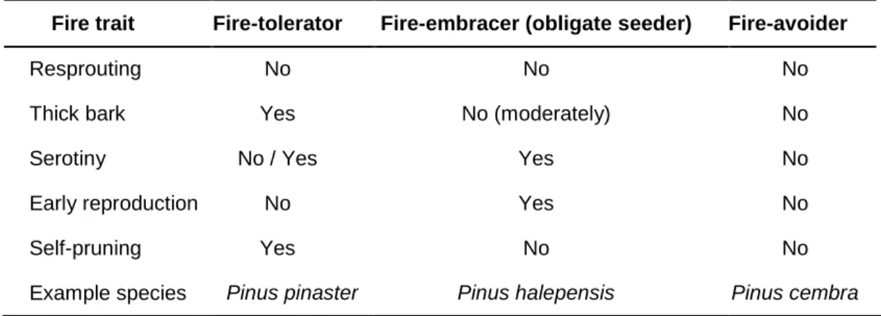
TABLE 1 | Main fire traits for each fire syndrome in pines 40
TABLE 2 | Overview of the structure of this thesis, including objectives, materials and methods, and results in form of publications and manuscripts
63
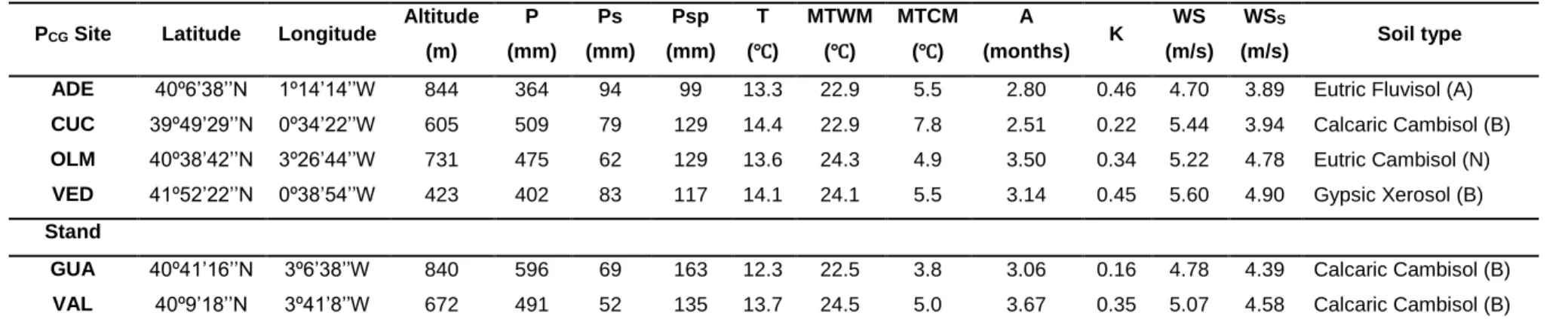
TABLE 3 | Description of the trial sites from the Pinus halepensis common garden experiment (PCG Site) and the two stands sampled to study maintenance costs of serotiny
(Study II)
69
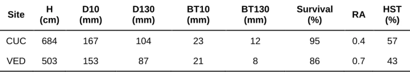
TABLE 4 | Mean values of different growth variables at both test sites. H: total tree height; D10: diameter at tree base (at 10 cm); D130: diameter at breast height (at 130 cm); BT10: bark thickness at tree base; BT130: bark thickness at breast height; Survival: percentage of tree survival; RA: reproductive allocation (10*number of female cones/tree height); HST: percentage of highly serotinous trees (those with > 80% of cones closed)
71
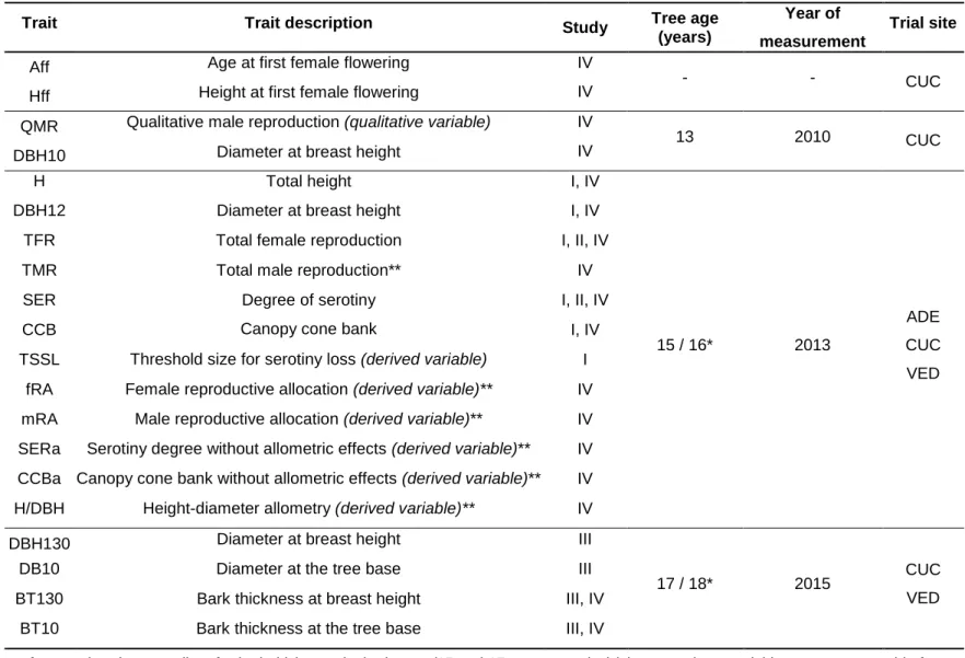
TABLE 5 | Summary of reported Pinus halepensis traits recorded in three contrasted sites of the common garden experiment
73
TABLE 6 | Summary of the samplings made at each site 81
TABLE 7 | Narrow-sense heritability and confidence intervals for family estimates reported in the literature for several traits for Pinus halepensis and Pinus pinaster. Heritability values in parenthesis are assumed values not from previous works (see above text for explanation). ‘Group’ indicates the three groups in which we have divided the heritability values according to their greater plausibility with respect to our data
96
TABLE 8 | Mean values and SE for the 11 traits studied in Pinus halepensis at the two experimental sites, and factor significance based on LMMs and GLMMs for each trait, including site, provenance and site x provenance (GxE) as fixed effects, as well as tree size to account for the allometric effect. Significance: ***P < 0.001, **P < 0.01, *P < 0.05
115
TABLE 9 | Correlations of trait population means with geographic and environmental variables at the populations’ origin, the two most important principal components from the environmental variables PCA and the natural fire frequency at populations’ origin. Data from both experimental sites pooled together. Cont.Index: continentally index; TCM: mean temperature of the coldest month; Psp: precipitation of the warmest quarter (spring); Ps: precipitation of the driest quarter (summer); Pa: precipitation of the wettest quarter (autumn); PDM: precipitation of the driest month; Lat: latitude; Long: longitude; Alt: altitude; FF: natural fires frequency
122
TABLE 10 | Correlations of trait population means with geographic and environmental variables at the populations’ origin, the two most important principal components from the environmental variables PCA and the natural fire frequency at populations’ origin. Data from the high-resource site (CUC)
8 from the low-resource site (VED)
TABLE 12 | Summary of the probability of QST > FST for each trait studied 127
TABLE S10.1.1 | Results from Principal Component Analysis applied to environmental data from 19 Pinus halepensis source populations. Variables with loadings > |0.80| in bold case
174
TABLE S10.2.1 | Bark allometric exponents (b) for bark volume of each population at the two experimental sites (confidence intervals in brackets). Significant P value indicates that b is different from 1 (isometric coefficient). r2 and significance for the standardized major
axis regression (SMA)
177
TABLE S10.3.1 | Geographic and climatic information about the 19 native populations of
Pinus halepensis used throughout this thesis
179
TABLE S10.3.2 | Number of trees from each population that were alive in 2013 at each of the four common garden sites used in this thesis
180
TABLE S10.3.3 | Cycle of controlled temperature and relative humidity used in the screening laboratory experiment with individual cones
182
TABLE S10.3.4 | Cycle of controlled temperature and relative humidity used in the manipulating water availability ex situ experiment with pairs of cones from the same whorl
182
TABLE S10.3.5 | Mean bark thickness and confidence intervals at breast height (BT130) and at the tree base (BT10) for each population and site (CUC: high-resources and VED: low-resources) obtained through general linear mixed models, and the calculated critical times for cambium kill, both at breast height (𝜏c130) and at the tree base (𝜏c10)
183
TABLE S10.3.6 | Correlations between mean bark thickness values (at breast height: BT130 and at tree base: BT10) from Pinus halepensis trees grown in a common garden experiment replicated in two contrasting sites (CUC: high-resources and VED: low-resources) and the first two Principal Components derived from a PCA analysis for nine environmental variables, as well as six environmental variables with PCA loadings > |0.80| representing average conditions in source populations. Significant correlations (< 0.10) are indicated in bold
184
TABLE S10.3.7 | Mean percentage of bark volume (%VB) and confidence intervals for each site and population (significant factors in the model) obtained through general linear mixed models
185
TABLE S10.3.8 | Variance explained by provenance for each phenotypic studied trait, pooling together data of both sites (CUC: high-resource and VED: low-resource). , for the high-resource site or for the low-resource site. Details about phenotypic traits in Table 5
9
TABLE S10.3.10 | Variance explained by provenance for each phenotypic studied trait, for data from the low-resource site (VED). Details about phenotypic traits in Table 5
187
TABLE S10.3.11 | Results from Principal Component Analysis applied to phenotypic traits data from 19 Pinus halepensis populations studied at the two experimental sites. Variables with loadings > |0.80| in bold case
191
TABLE S10.3.12 | Results from the PCA applied to phenotypic traits data from 19 Pinus halepensis populations studied at the high-resource site (CUC). Variables with loadings > |0.80| in bold case
193
TABLE S10.3.13 | Results from the PCA applied to phenotypic traits data from 19 Pinus halepensis populations studied at the low-resource site. Variables with loadings > |0.80| in bold case
195
TABLE S10.3.14 | Correlations coefficients and significance of the correlation at the population level between raw data of the studied phenotypic traits at each experimental site and the Gower’s distance to each site
196
TABLE S10.3.15 | Correlations coefficients and significance of the correlation among the eight original environmental variables (before selection) and the three geographical variables from the origin of the 19 P. halepensis populations used in this thesis
197
TABLE S10.3.16 | Global phenotypic differentiation among populations (QST) with its
confidence intervals (CI) for Pinus halepensis provenances grown in a high-resource site (CUC) of a common garden experiment, the narrow-sense heritability values (h2) used for
QST calculation (see Table 7) and QST - FSTcomparison. QST - FSTcomparisons have been
made comparing both the CIs and the distribution of values (always P < 0.0001 in the Kruskal-Wallis chi-squared)
198
TABLE S10.3.17 | Global phenotypic differentiation among populations (QST) with its
confidence intervals (CI) for Pinus halepensis provenances grown in a low-resource site (VED) of a common garden experiment, the narrow-sense heritability values (h2) used for
QST calculation (see Table 7) and QST - FSTcomparison. QST - FSTcomparisons have been
made comparing both the CIs and the distribution of values (always P < 0.0001 in the Kruskal-Wallis chi-squared)
11
FIGURE 1 | Forest area as a percentage of total land area in 2015 27
FIGURE 2 | Surface covered by forests in Europe in 2011. Information based on remote sensing technologies and forest inventory statistics
28
FIGURE 3 | World biodiversity hotspots 28
FIGURE 4 | Serotinous structures of different genera and species: (A) Leucadendron salicifolium (Proteaceae), (B) Leucadendron rubrum (Proteaceae), (C) open burned serotinous cone of Banksia sp. (Proteaceae), (D) Cupressus macrocarpa (Cupressaceae), (E) Pinus radiata (Pinaceae), (F) Pinus rigida (Pineaceae), (G) Pinus pinaster (Pinaceae) and (H) Pinus halepensis (Pinaceae)
43
FIGURE 5 | Diversity of bark among species: (A) Persoonia linearis (Proteaceae), (B)
Alstonia actinophylla (Apocynaceae), (C) Bursera instabilis (Burseraceae), (D) Exocarpus cupressiformis (Santalaceae), (E) Eucalyptus tenuiramis (Myrtaceae), (F) Eremanthus seidelii (Asteraceae), (G) Myrcia bella (Myrtaceae), (H) Quercus suber (Fagaceae), (I-J) are different populations of Pinus halepensis (Pinaceae) and (K) Byrsonima verbascifolia
(Malpighiaceae). (L-P) Cross-sectional variation in bark thickness: (L) Buchanania obovata (Anacardiaceae), (M) Brachychiton paradoxus (Malvaceae), (N) Lophostemon lactifluus (Myrtaceae), (O) Planchonia careya (Lecythidaceae), (P) Alstonia actinophylla
(Apocynaceae)
47
FIGURE 6 |Bark structure in cross-section 48
FIGURE 7 | (A) Representation of the chimney effect in trunks, (B) photograph showing the chimney effect in a prescribed burn
51
FIGURE 8 | Phylogenetic tree for the seven Mediterranean pine species and for an American outgroup, with the group P. halepensis-P. brutia identified
53
FIGURE 9 | Pinus halepensis distribution map. Blue shaded areas correspond to the species natural distribution
55
FIGURE 10 | (A) Needles, (B) immature male cones, (C) winged small seeds and (D) female cones of Pinus halepensis
57
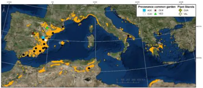
FIGURE 11 | Distribution map of Pinus halepensis source populations (black and grey points -grey points are two populations not used in Chapter 4-), and all sites used in this thesis. Four sites from a common garden experiment (ADE, CUC and VED were used in
Study I, CUC and OLM in Study II, CUC and VED in Studies III and IV) and two plant stands used also in Study II. Orange areas indicate the species’ natural distribution range
12
planted with the same provenance plant stock and following the same methods
FIGURE 13 |Scheme of the average tree at each of the test sites. H is the total height of the tree. Diameters and bark thicknesses of the circular cross-sections were measured at 10 and at 130 cm from the ground. This scheme does not represent the real decrease in diameter and bark thickness along the trunk above 130 cm due to the lack of measurements at higher heights. This decline is neither constant nor homogeneous
70
FIGURE 14 | Core extraction process to assess tree age by ring-counting in the plantations. (A) Pressler bit (increment borer), (B) detail of core extraction, (C) complete extraction of the core and (D) core placed for ring-counting in the laboratory
72
FIGURE 15 | Measuring total height and diameter of a Pinus halepensis tree. (A) Telescopic pole used for measuring total height and (B) detailed of the telescopic pole. (C-D) Caliper used for measuring diameter
74
FIGURE 16 | Pinus halepensis female cone developmental stages and male cone clusters. (A) Female strobili emerged in spring, (B) one-year old female conelets, (C) two-year old female cone, (D) serotinous cone and (E) immature male cone clusters
75
FIGURE 17 | (A) Photograph of a standard bark gauge, (B) measuring bark thickness with the bark gauge and (C) standard bark gauge indicating the thickness of the measured bark
77
FIGURE 18 | Determination of cone age by counting wood rings at the branch section just below of the cone insertion (Tapias et al., 2001)
82
FIGURE 19 | (A) Obtaining central scales of a Pinus halepensis cone and (B) measuring the hydrostatic thrust of the submerged scales in water to calculate their volume
83
FIGURE 20 | Description of the in situ manipulative experiment. (A) Pair of closed serotinous cones of the same whorl of P. halepensis. The thick and long peduncles characteristic of this species are easily distinguishable. (B) ‘Closed’: both branched and detached cones of the pair remained closed; (C) ‘Positive’: detached cone opened earlier than its branched pair; (D) ‘Negative’: detached cone opened later than its branched pair; (E) ‘Opened’: both cones of the pair opened between observations. b, branched cone -control-; d, detached cone
84
FIGURE 21 | Manipulating water availability in the ex situ experiment. Scheme of the experiment inside the Styrofoam box. W, watered cones; L, waterless cones
13
with closed cones recently placed inside the controlled conditions chamber. An aluminum film cover was used to further increase isolation and prevent water heating. (E) Photograph of the experiment in progress. There are few cones already open and the others are still closed
FIGURE 23 |Total and bark volumes of the cone trunk from the tree base to breast height. Scheme used for studying allometry of bark allocation
91
FIGURE 24 | Biplot of (A) average tree height and survival rate and (B) tree height and total female cones at the three P. halepensis trial sites (blue square: ADE −cold site−; red triangle: VED −dry site−; green circle: CUC −mild site−). In (A), letters indicate homogeneous groups for height and letters in italics for survival. In (B), letters indicate homogeneous groups for total female cones and insert values correspond to the ratio between cone number and tree size (cones per cm of height)
99
FIGURE 25 | Frequency distributions of degree of serotiny per trial site of Pinus halepensis. ADE is the cold site, CUC is the mild site, and VED is thedry site
100
FIGURE 26 | Logistic models relating degree of serotiny to tree height in Pinus halepensis
trees grown at three contrasting trial sites. Data include range-wide populations and are thus representative of the whole species. Solid line corresponds to ADE −cold site−, dashed line corresponds to VED −dry site− and dot-dash line corresponds to CUC −mild site−. Gray lines and shades represent the upper and lower 95% credible intervals of each model
101
FIGURE 27 | Representation of the genotype x environment interaction in the degree of serotiny without taking into account the tree size effect. ADE: cold site, CUC: mild site, and VED: dry site. Numbers indicate provenances (see Table S10.3.1 for information about provenances)
102
FIGURE 28 | Representation of the genotype x environment interaction in the TSSL. Populations shown are among the few in which the models adjusted for both sites and were significant. Comparison between ADE and VED sites was not possible because there were no fitted models for the same population on both sites. ADE is the cold site, CUC is the mild site and VED is the dry site
103
FIGURE 29 | (A) Mean canopy cone bank for 19 range-wide populations of Pinus halepensis. (B) Model estimates and confidence intervals for canopy cone bank at the three contrasting trial sites (ADE -cold site-, CUC -mild site- and VED -dry site-)
14
and (B) peduncles show living cortical tissues (phloem and cortical parenchyma), but not (C). 99% of P. halepensis cones sampled in this study were in the ‘(A)’ status. (D) Section
of the peduncle close to the tree branch of one of the few P. halepensis cones with heartwood. (E) Longitudinal section of a P. halepensis cone. The peduncle shows a light colored sapwood with connection to the cone scales
FIGURE 31 | Frequency distribution (A) for temperature of cone opening and (B) for density of the scales of the cones in the laboratory screening experiment
106
FIGURE 32 | Cone opening by treatment for the manipulating water availability ex situ experiment. Categories meaning is the following: ‘Positive’, cones opened after its pair, i.e. cones remained closed longer; ‘Negative’, cones opened before its pair; L, waterless cones; W, watered cones
107
FIGURE 33 | Cone opening at OLM site by provenance and treatment. (A) Percentage of cone opening for some provenances with contrasting behavior pertaining to the two different provenance groups. Provenances 152 and 158 are part of the Northeast group; provenances 172 and 241 are part of the Southwest group. This plot illustrates the significant treatment by provenance interaction found at this site. (B) Percentage of cone opening during the experiment at OLM site, by treatment. Brown shadows indicate summer seasons. b, branched cones -control-; d, detached cones
108
FIGURE 34 | Progress of the field manipulative experiment at OLM site from 10 to 125 weeks after its setting up. Categories meaning is the following: ‘Close’, both cones of the pair remained closed; ‘Positive’, the detached cone opened earlier; ‘Negative’, the attached cone opened earlier; ‘Open’, both cones opened between observations. Numbers in the bars correspond to the significance of McNemar's test
109
FIGURE 35 | A) Bark thickness vs sapwood diameter of P. halepensis populations at each experimental site. BT130 and BT10 are bark thickness at breast height and at the tree base, respectively; SD130 and SD10 are sapwood diameter at breast height and at the tree base, respectively. Horizontal black lines represent the assumed values of critical bark thickness for cambium survival (solid line: 10 mm; dashed-line: 20 mm). Numbers indicate the critical time for cambium kill (𝜏c) for some divergent populations (Table S3). Significance for Spearman correlations between bark thickness and sapwood diameter at: ***P < 0.001, **P < 0.01, *P < 0.05, n.s. = no significant. B) Variation between sites of the relationship between critical bark thickness and sapwood diameter of three representative
P. halepensis populations
111
FIGURE 36 | Percentage of bark volume vs. total volume per site for the mean total volume of the cone trunk from the tree base to breast height -between 10 and 130 cm height- (16.8 dm3), and the minimum and maximum total volume (~3 dm3 and ~52 dm3,
respectively). At higher total volume, the differences between sites are magnified. Green line represents CUC site –mild conditions and high resource availability– and orange dashed-line is VED site –dry conditions and low resource availability–
15
FIGURE 38 | Plots indicating phenotypic integration in Pinus halepensis. A) Data for both sites together. B) Correlations at the high-resource site (CUC site). C) Correlations at the low-resource site (VED site). Solid lines indicate positive correlation, dashed lines indicate negative correlation. Line thickness is proportional to the significance level (***P < 0.001, **P < 0.01, *P < 0.5, ·P < 0.1). Colours group traits in functional groups: growth traits in blue color, fire-adaptive traits in red colour and reproductive traits in green colour
118
FIGURE 39 | PCAs based on population trait means in Pinus halepensis for (A) the 11 phenotypic traits studied at both sites, (B) the 15 traits studied at the high-resource site (CUC site) and (C) the 13 traits studied at the low-resource site (VED site). Red circle group the Tunisian and southern Spain populations; green circle cluster the Greek populations, and yellow circle bunch some of the northern Spanish populations
119
FIGURE 40 | Gower’s (absolute) environmental distance between each population to the location of the two sites of the common garden. Circles indicate distance to CUC site (favorable environment) and triangles indicate distance to VED site (harsh environment)
120
FIGURE 41 | Among-population differentiation (QST) calculated for different heritability
values (h2) for the traits studied in 19 Pinus halepensis populations growing in two trial
sites with contrasting environmental conditions (CUC in green colour, VED in orange colour). Grey line indicates mean FST. Meaning of trait abbreviations as in Table 5. Graphs
for MR and mRA shows qualitative data for 2010 at CUC site and quantitative data for 2015 at VED site. Aff and Hff were just measured at CUC site. Heritability values in bold case are from group 1 according to their greater plausibility with respect to our data, h2
values in italics belong to group 2, h2 in black belong to group 3 and h2 in grey colour are
assumed values (see Table 7)
126
FIGURE 42 | Biplots of the canopy cone bank (CCB) against degree of serotiny among range-wide Pinus halepensis provenances (r = 0.67**). A) Bubble size represents female fecundity, through classes of total number of female cones produced during 16 years. Female fecundity is highly correlated with CCB (r = 0.93***). B) Bubble size represents classes of ages at first reproduction which is negatively correlated with CCB (r = -0.74***)
131
FIGURE S10.1.1 | Scree plot for the PCA of the nine environmental variables 173
FIGURE S10.3.1 | Representative map of the Spanish genetic trial network for Pinus halepensis and aerial photographs of the four common garden sites used throughout this thesis
16
adaptive traits and green box grouped reproductive traits. Below diagonal, graphical pairwise relationships are shown and above diagonal, pairwise Pearson’s correlation coefficients and level of significance of the correlation (***P < 0.001, **P < 0.01, *P < 0.5, ·P < 0.1)
FIGURE S10.3.3 | Graphical pairwise correlations, correlation coefficients and significance of the correlation at the population level for the 15 studied phenotypic traits at the high-resource site (CUC site) in Pinus halepensis. Blue box marks growth traits, red box indicates fire-adaptive traits and green box grouped reproductive traits. Below diagonal, graphical pairwise relationships are shown and above diagonal, pairwise Pearson’s correlation coefficients and level of significance of the correlation (***P < 0.001, **P < 0.01, *P < 0.5, ·P < 0.1)
189
FIGURE S10.3.4 | Graphical pairwise correlations, correlation coefficients and significance of the correlation at the population level for the 13 studied phenotypic traits at the low-resource site (VED site) in Pinus halepensis. Blue box marks growth traits, red box indicates fire-adaptive traits and green box grouped reproductive traits. Below diagonal, graphical pairwise relationships are shown and above diagonal, pairwise Pearson’s correlation coefficients and level of significance of the correlation (***P < 0.001, **P < 0.01, *P < 0.5, ·P < 0.1)
190
FIGURE S10.3.5 | Scree plot for the PCA of the eleven phenotypic traits studied at both sites. This figure revealed that two principal components should be retained
190
FIGURE S10.3.6 | Scree plot for the PCA of the fifteen phenotypic traits studied at the high-resource site (CUC). This figure revealed that two principal components should be retained
192
FIGURE S10.3.7 | Scree plot for the PCA of the thirteen phenotypic traits studied at the low-resource site (VED). This figure revealed that three principal components should be retained
17
Structure of the Thesis
This thesis is based on two original works published in different international journals and two other manuscripts under preparation. The text is written in English and includes a thesis overview, an abstract, an introduction with the hypothesis and objectives of the thesis, a materials and methods section, describing in detail the different sampling sites and phenotyping procedures used to obtain pine phenotypes of different life-history traits in Pinus halepensis, a results section, a general discussion and conclusions. In addition, we have included a final section with future perspectives and gaps of knowledge regarding the topics studied in this thesis. The abstract and the conclusions are written both in English and in Spanish language. Finally, supplementary information with additional tables and figures for the thesis are included.
19
Abstract
Forests have high ecological, economic and social value, besides playing a key role in the maintenance of biodiversity and as carbon sinks, but the current global change can cause adaptation problems of forest species as well as modify forests distribution and functioning. Mediterranean environments are especially sensitive to climate change, where predictions suggest that temperature increase and rainfall decrease will be especially drastic, together with a higher frequency and intensity of disturbances (forest fires and epidemic outbreaks of pests and diseases). The scarce availability of water is the most evident resource limitation in these Mediterranean environments and may increase the evolutionary trade-offs among vital functions predicted by the life-history theory. This theory is based on the idea that forest trees, like other living beings, must optimize the amount of energy and resources they dedicate to each of their vital functions since the available resources are limited.
Pine trees are long-life large organisms with short age at first reproduction and several advantages for the study of adaptive traits in trees from an ecological-evolutionary approach. Mediterranean pine forests constitute reservoirs of adaptive genetic diversity of great value in the face of environmental change. The ability of those populations to persist in the medium term will depend to a large extent on the existence of sufficient genetic variation in relevant traits, on the exchange of genetic information among populations (genetic flow) and on their adaptive phenotypic plasticity. Local adaptation is expected to arise from genetic variability within and between populations, but phenotypic plasticity also plays a major role in the ability of species to cope with environmental changes and may allow the appearance of adapted phenotypes without the existence of an underlying genetic change. However, knowledge about the adaptive role and the plasticity of key life-history traits is still very limited in forest species, especially in Mediterranean environments. Among the life-history traits stand out the reproductive ones, such as the threshold size of reproduction or fecundity, but serotiny degree or bark thickness are other fundamental traits related to adaptation to fire that have received so far less attention.
20
compromises among adaptive traits (life-history traits) in a typical Mediterranean pine (Pinus halepensis Mill., Aleppo pine), which can be considered a model of maximum resilience in Mediterranean ecosystems. Specifically, we focused on two key resilience traits: serotiny of female cones to build an aerial seedbank that ensures regeneration after intense crown fires, and bark thickness that allows survival of adult trees in front of less severe fires until reaching a sufficient aerial seedbank, without forgetting its interrelation with other traits such as reproduction (female and male) or growth. Both traits are complementary but not mutually exclusive. Understanding their genetic and environmental variation patterns, unraveling the complex interaction between genotype, phenotype and environment, together with the allometric effects (ontogenetic or developmental), constitutes a fundamental challenge to be able to foresee the response of these forests under the new environmental scenarios, and for the management and conservation of forest resources under the current global change. The use of provenance trials in contrasted common environments allowed us to separate the genetic effects from environmental effects and interacting developmental differences. In addition, climatic and fire information from the populations’ origin areas was used to identify ecotypic patterns of variation.
Throughout the different studies involved in this thesis, we found clear evidence of intraspecific genetic variation and high phenotypic plasticity, as well as genotype-by-environment interaction and signs of local adaptation in the different studied traits. This suggests the existence of potential evolutionary change to face new selective pressures, variable within the species distribution range. The quantitative genetic differentiation between populations was higher than the differentiation found with molecular markers for fire-adaptive traits under contrasting environments. The growth-limiting environments for P. halepensis, mainly continental conditions with high annual and/or daily thermal
oscillation that reduce the vegetative period, and the shortage of precipitations in spring and summer, accelerated the early release of seeds and decreased the allocation to bark.
21
the duration of serotiny in P. halepensis implies the supply of water to the cones through its peduncles by the bearing plant, which suggests the existence of maintenance costs of serotiny.
We verified the existence of phenotypic plasticity and allometric plasticity in bark thickness, a fire-adaptive trait poorly studied in conifer species. Confirming our hypothesis environments with lower resource availability limited both the relative allocation to the bark and absolute bark thickness. Importantly, this can increase immaturity risk in P. halepensis populations (death by moderately intense fires before reaching an aerial bank of seeds that ensures regeneration) under the dryer environments caused by climate change.
We also studied the relationship between ecogeographic variables and different adaptive phenotypes in P. halepensis -including growth, female and male reproduction and fire-adaptive traits-, as well as the correlations among traits. In general, we found evidence of local intraspecific adaptation. We also confirmed that trade-offs in terms of allocation of resources to adaptive traits related to growth, reproduction and defense against fire matched the predictions of life-history theory and differential allocation. Finally, further confirming the hypothesis of local adaptation, we verified that the quantitative genetic differentiation among populations was greater than the neutral genetic differentiation for serotiny and bark thickness.
23
Resumen
Los bosques tienen un alto valor ecológico, económico y social, además de desempeñar un papel clave en el mantenimiento de la biodiversidad y como sumideros de carbono, pero el cambio global actual puede causar problemas de adaptación de las especies forestales al igual que modificar la distribución y el funcionamiento de los bosques. Los ambientes mediterráneos son especialmente sensibles al cambio climático, donde las predicciones sugieren que el aumento de la temperatura y la disminución de las lluvias serán especialmente drásticos, junto con una mayor frecuencia e intensidad de las perturbaciones (incendios forestales, y epidemias de plagas y enfermedades). La escasa disponibilidad de agua es la limitación de recursos más evidente en estos entornos mediterráneos, pudiendo acrecentar los compromisos evolutivos entre funciones vitales predichos por la teoría de historia vital. Esta teoría se basa en que los árboles forestales, al igual que el resto de seres vivos, deben optimizar la cantidad de energía y recursos que dedican a cada una de sus funciones vitales, ya que los recursos disponibles son limitados.
24
Esta tesis se enmarca en el campo de la ecología evolutiva e incluye cuatro estudios que corresponden a artículos científicos ya publicados o manuscritos en preparación. Incluye también diversos anexos con información adicional. El objetivo principal de este trabajo fue comparar cómo distintos ambientes más o menos favorables condicionan los compromisos entre caracteres adaptativos (rasgo del ciclo de vida) en un típico pino mediterráneo (Pinus halepensis Mill., pino carrasco), que puede considerarse un modelo de máxima resiliencia en los ecosistemas mediterráneos. En concreto, nos hemos centrado en dos caracteres de resiliencia claves: la serotinia de los conos femeninos para construir un banco aéreo de semillas que asegure la regeneración tras fuegos de copas intensos, y el espesor de corteza que permite la supervivencia de los árboles adultos frente a incendios menos severos hasta alcanzar un banco aéreo de semillas suficiente, sin olvidar su interrelación con otros caracteres como la reproducción (femenina y masculina) o el crecimiento. Ambos caracteres son complementarios pero no excluyentes. Comprender sus patrones de variación genética y ambiental, desentrañando la compleja interacción entre genotipo, fenotipo y ambiente, junto con los efectos alométricos (ontogénicos o de desarrollo), constituye un reto fundamental para poder prever la respuesta de estos bosques bajo los nuevos escenarios ambientales, y para la gestión y conservación de los recursos forestales bajo el cambio global actual. El uso de ensayos de procedencias en ambiente común (common gardens) y contrastados entre sí, nos ha permitido separar los efectos genéticos de los ambientales y de los puramente debidos al desarrollo. Además, la información climática y de incendios de las áreas de origen de las poblaciones se utilizó para identificar patrones de variación ecotípicos.
25
verano, aceleraron la liberación precoz de semillas y disminuyeron la asignación a la corteza.
El estudio pormenorizado del grado de serotinia de P. halepensis persiguió por un lado, determinar la plasticidad fenotípica de la serotinia teniendo en cuenta los efectos alométricos y genéticos, y por otro lado, examinar si existen o no factores endógenos que puedan afectar a la apertura de los conos serótinos. Para ello, las mediciones en los ensayos de procedencias se completaron con experimentos manipulativos en laboratorio y campo. Encontramos que los ambientes desfavorables para el crecimiento causaron la liberación precoz de semillas y que la duración de la serotinia en P. halepensis implica el suministro de agua a los conos a través de sus pedúnculos por parte de la planta, lo que sugiere la existencia de costes de mantenimiento de la serotinia.
Verificamos la existencia de plasticidad fenotípica y plasticidad alométrica en el espesor de corteza, un rasgo de adaptación al fuego poco estudiado en especies de coníferas. Confirmando nuestra hipótesis, los entornos con menos disponibilidad de recursos limitaron tanto la asignación relativa a la corteza como el grosor absoluto de corteza. Es importante destacar que esto puede aumentar el riesgo de inmadurez en las poblaciones de P. halepensis (muerte por incendios moderadamente intensos antes de llegar a un banco aéreo de semillas que garantice la regeneración) en lo ambientes más secos causados por el cambio climático.
También estudiamos la relación entre variables ecogeográficas y diferentes fenotipos adaptativos en P. halepensis -incluyendo crecimiento, reproducción femenina y masculina y caracteres de adaptación al fuego-, así como las correlaciones entre caracteres. En general, encontramos evidencia de adaptación local intraespecífica. También confirmamos que las compensaciones en términos de asignación de recursos a los caracteres adaptativos relacionados con crecimiento, reproducción y defensa contra el fuego coincidían con las predicciones de la teoría de historia vital y la asignación diferencial. Finalmente, confirmando de nuevo la hipótesis de adaptación local, verificamos que la diferenciación genética cuantitativa entre poblaciones fue mayor que la diferenciación genética neutra para la serotinia y el espesor de corteza.
26
27
1.
Introduction
1.1.
Forest ecosystems and climate change
Forests occupy 30.6 % of the Earth's surface (FAO 2015; Figure 1) and are critical points of biodiversity (Myers et al., 2000). Forests provide fundamental ecosystem services such as water regulation and supply, generation, renewal and maintenance of soil, purification of air, mitigation of the effects of droughts and floods, pollution control, etc. (Daily, 1997; FAO, 2015). In addition, they are a source of oxygen fundamental for life on Earth, as well as important carbon sinks, becoming key elements for the mitigation of anthropogenic climate change (Canadel and Raupach, 2008). Forest ecosystems are also useful for the economy and for the subsistence of millions of people, since they are the source of many highly demanded products such as food, medicines, wood, resin or cork. Although the rate of net forest loss has decreased lately, there is still an annual net reduction in the forest area of 3.3 million hectares per year (period 2010-2015; FAO, 2015), with the greatest losses in the tropics. In contrast, in other regions such as Europe, deforestation rates are decreasing and forest area is even increasing. Currently, forests cover nearly 40% of the European Union surface (Figure 2).
Mediterranean forests stand out for their high biodiversity, as a result of a noteworthy variety of habitats and of the historical and paleogeographic episodes mainly occurring during the last glaciation. Consequently, the Mediterranean basin that hosts most of the Mediterranean forests in the world, has been identified as a biodiversity hotspot (Myers et al., 2000; Mittermeier et al., 2011; Figure 3).
28
FIGURE 2 | Surface covered by forests in Europe in 2011. Information based on remote sensing technologies and forest inventory statistics. From European Forest Institute (http://www.efi.int/) and Kempeneers et al. (2011).
29
Climate change is mainly characterized by increasing air temperature and changing precipitation regimes (IPCC, 2013) and is becoming one of the most important challenges faced globally by ecosystems and societies (see for example, Thomas et al., 2004; Thuiller, 2007; Bernier and Schöne, 2009). Moreover, climate change potential consequences could be worsened by already existing human-induced threats such as the introduction of exotic pests and pathogens, habitat degradation and fragmentation, land-use changes or modifications in wildfire regimes (Blondel et al., 2010; Keenan, 2015). In this context, forest ecosystems seem to be particularly vulnerable as the long life-span of trees can limit rapid adaptation to environmental changes and their sessile nature restricts natural migration (Lindner et al., 2010). This can put at stake forest resilience, i.e. the capacity to resist disturbances recovering after them and maintaining its structure and function (sensu Lloret et al., 2011). Specifically, Mediterranean forest ecosystems are generally expected to be
particularly vulnerable to climate change (IPCC, 2007; Lindner et al., 2010) due to the expected increase in the frequency of extreme events such as droughts and fires, which are likely to be more severe in dry, high-temperature regions (IPCC, 2007).
In the face of all these numerous drivers of global change, species can persist, either migrating to new ecological niches or adapting to new conditions in current locations or, on the contrary, become extinct locally (Aitken et al., 2008). Forests are resilient, their distribution ranges are highly dynamic and many tree populations maintain high genetic diversity, so they are expected to adapt rapidly. However, environmental variations under current climate change are of such magnitude or will occur at speeds much higher than the natural adaptive capacity of forest species, possibly jeopardizing their persistence (Petit and Hampe, 2006; Petit et al., 2008; Milad et al., 2011). The persistence of tree species under forecasted climate change scenarios will depend on their genetic diversity and their phenotypic plasticity, which plays a major role in the response of plant populations to environmental changes (Matesanz et al., 2010; Valladares et al., 2014). Therefore, understanding the past adaptive processes in forest tree species, and how forests can resist and recover after extreme climatic events or intense perturbations across different regions is key to predict the future responses of forests to climate change (see for example, Savolainen et al., 2007; Petit et al., 2008).
30
is essential to understand the causes of variation (genetics, plasticity, allometry-ontogeny...) affecting to species' life-history traits, and particularly, to fire-adaptive traits. Likewise, it is key to consider the possible existence of ecotypic patterns, local adaptation or trade-offs among fire-adaptive traits and other characters related to other vital functions such as reproduction or growth. In this thesis, we have tried to solve the gaps of knowledge related to these aspects, taking as study species a Mediterranean pine with high resilience.
1.2.
Genetic variation
Genetic variation is a fundamental requirement for the variability of species, populations and ecosystems (Allendorf and Luikart, 2007), and for the existence of evolutionary adaptation enabling species adaptation to environmental changes (Le Corre and Kremer, 2003), in addition to being considered the most basic level of biological diversity. While different processes (mutation, genetic drift and migration) generate or deplete genetic variation stochastically, speeding up or constraining adaptation, natural selection is the only evolutionary force that is considered to lead to adaptation due to its directional nature even taking into account that it can also limit genetic variation. For phenotypes to evolve, it is essential that the particular trait shows heritable variation. Natural selection acts on this variation, selecting phenotypes with higher fitness. Genetic changes might modify the average phenotype in the population across generations, possibly improving the population fitness and thus, leading to adaptation (Le Corre and Kremer, 2003). However, there is increasing evidence that adaptation can be also shaped by phenotypic changes that do not imply changes in the genotype, but in environmentally driven modifications of gene expression (epigenetics), since epigenetic changes can be transmitted among generations (Duncan et al., 2014).
31
detected at molecular or phenotypic level. Population genetics deals with the dynamics of allele frequencies both within and among populations under the influence of evolutionary forces such as drift, mutation, selection or migration. However, genes underlying many phenotypic traits are still unknown, especially in forest species, so this approach often fails to consider phenotypes. Lately, advances in genotyping have improved the characterization of genomes reducing costs and time needed, but in contrast accurate phenotyping is still costly in money and time (Ingvarsson and Street, 2011). Quantitative genetics concentrates on how individual variation in genotype and environment contribute to the variance in phenotype. Most key adaptive plant traits are quantitative and polygenic (Mackay et al., 2009, Pritchard et al., 2010). The statistical techniques normally used to analyze quantitative genetic data assume that traits follow a Gaussian distribution, which is generally true for growth-related traits, but not true for other life-history traits such as reproduction or serotiny. This hinders the analysis of the data. However, in recent years, new statistical techniques have been implemented in quantitative genetics improving parameters estimation (see Nakagawa and Schielzeth, 2010, Holand et al., 2013, Appendix VI in Santos-del-Blanco, 2013).
Genetic adaptive variation patterns could be confounded with variation trends due to demo-stochastic processes. These processes, together with natural selection, model the species population genetic structure (Box 1; Freedman et al., 2004). This could render the study of polygenic traits in natural populations more difficult. Recently, statistical techniques have been developed that take population genetic structure and inter-individual relatedness into account (Yu et al., 2006, Eckert et al., 2010).
Box 1. Spatial Genetic Structure
32
1.3.
Phenotypic plasticity
Environmental differences cause phenotypic variation (growth rates, shape, morphology, etc.) among neighboring individuals (caused by differences in microclimate, microsite, competition and exposure to insects and diseases) and also in populations of the same species growing in different environments (caused by differences in elevation, precipitation, temperature regimes, soil type, etc.; White et al., 2007). Leaving aside the non-additive genetic effects, the observed phenotypic value of a quantitative (i.e. polygenic) trait results from the sum of three components: genotype (G), environment (plasticity, E) and their interaction (P = G + E + G x E). Phenotypic plasticity is ultimately an individual property (Stearns, 1989a; West-Eberhard, 2003 and many more). Therefore, it is considered that for phenotypic plasticity to be adequately addressed, it must be studied with replicated genotypes, that is, with experiments that use the same genotype (clones) or individuals with a known genetic relationship (genetic families) (Såstad et al., 1999; Richards et al., 2006; Herrera, 2009). However, populations or even species can also be used as experimental subjects for research on phenotypic plasticity (Pigliucci 2001; Valladares et al., 2006; Richards et al., 2006; and Gianoli and Valladares 2012 for a review) when the objective seeks to find differences in plasticity along an environmental gradient (see, for example Gianoli and González-Teuber, 2005; Bell and Galloway, 2008). In addition, this broad approach to plasticity allows the inclusion of more study units.
In recent years, phenotypic plasticity and its adaptive role for a plethora of traits have received huge interest by the scientific community, mainly due to its critical role in the response of plant populations to climate change, putatively allowing adaptation without genetic changes (Aitken et al., 2008; Matesanz et al., 2010; Chevin et al.; 2012, Valladares et al., 2014). Phenotypic plasticity can be defined as the environmentally induced variation
33
conditions remain unknown (Nicotra et al., 2010). In population genetic studies, counter-gradient variation patterns, i.e. phenotypic and genetic clines exhibiting opposing directions (unlike the most common co-gradient variation patterns where phenotypic and genetic variation show parallel responses to environmental gradients) can interfere with the processes of adaptive differentiation (Conover and Schultz, 1995; Kremer et al., 2014). Despite the importance of phenotypic plasticity for plant adaptive traits, many studies continue to mix genetic variation with phenotypic plasticity (Chambel et al., 2007). Besides, the use of experimental approaches as common gardens can avoid phenotypic differences due to genotype x environment interactions.
Genotype-by-environment interaction (G × E), i.e. genetic variation in phenotypic plasticity among populations (Schlichting, 1986), is a central concept in ecology and evolutionary biology because it has wide-ranging implications for trait development and for understanding how organisms will respond to environmental change. Genotypes performance commonly varies across environments leading to variance differences and rank changes among genotypes (Cooper and DeLacy 1994). Importantly, we should distinguish between two types of G x E (El-Soda et al., 2014; Heslot et al., 2014; Roles et al., 2016; Saltz et al., 2018). On the one hand, the biologically more relevant cross-over
34
It is well established that many phenotypic traits in plants vary as a function of growth and development, which are also highly plastic. So conclusions regarding phenotypic plasticity can dramatically change if developmental, i.e. ontogenetic differences are taken into account (Wright and McConnaughay, 2002; Valladares et al., 2006). Assessing the covariation of a given trait with body size (allometry) is routinely used to unveil the ontogenetic component of plasticity (Wright and McConnaughay, 2002; Weiner, 2004). Meaningfully, there is evidence that several traits variation have an allometric component in different plant species, although the direction of this trend could vary among genera (Cowling and Lamont, 1985; Sultan, 2000; Thanos and Daskalakou, 2000; Niklas and Enquist, 2003; Weiner et al., 2009, Bonser et al., 2010, Anderson et al., 2012, Tonnabel et al., 2012, Santos-del-Blanco et al., 2013 and many others). Resource allocation in plants changes along ontogenetic trajectories; therefore, distinguishing between environmental effects from purely developmental differences is critical when studying plasticity in allocation (Poorter and Nagel, 2000; Wright and McConnaughay, 2002; Weiner, 2004). While accounting for ontogenetic changes in such complex plants as adult trees is elusive, the concepts and theory of allometry are probably the best available tools. There are different strategies to study plant allometric patterns, all of them with advantages and disadvantages (Poorter and Sack, 2012). However, allometric equations is the most common method. Usually, these equations are in the form of a logarithmically-transformed power law (Niklas, 1994, Ter-Mikaelian and Korzukhin, 1997).
1.4.
Local adaptation
35
produced by a local allelic shift that maximizes fitness in a specific environment. This usually occurred during the expansion of the species since by expanding their geographical range, species faced new selective pressures that act on phenotypic variation and thus, on genetic variation. However, human-driven climate change will impose stronger and faster selection pressures (Davis and Shaw, 2001), challenging local adaptation processes in tree species (reviewed in Savolainen et al., 2013).
Long-lived tree species are often found in large natural populations (connected by extensive gene flow) and occupy large geographical distributions covering different environmental gradients, enabling the study of local adaptation processes, the possibilities of tree populations to adapt to changing environments and disentangling selective from stochastic evolutionary forces (Petit and Hampe 2006; Neale and Kremer 2011). Forest tree populations generally show high levels of genetic variation, phenotypic plasticity and genotype-by-environment interaction for various adaptive traits, which increases their capacity for adaptation and resilience (Sgrò et al., 2011; Fady et al., 2015) and is usually interpreted as indicative of local adaptation (Howe and Aitken, 2003; Petit and Hampe, 2006; Bucci et al., 2007; Savolainen et al., 2007; Petit et al., 2008; Grivet et al., 2011; Santos-del-Blanco et al., 2012; Alberto et al., 2013). Tree species ability to adapt depends on their genetic diversity, phenotypic plasticity, selection pressure, fecundity, interspecific competition and biotic interactions (Aitken et al., 2008). Local adaptation could be confounded with neutral genetic effects, plasticity or maternal effects (Savolainen et al., 2013). Discriminating between phenotypic plasticity and genetic divergence requires the measurement of traits in individuals from different populations under comparable (and different) environmental conditions (i.e. tested in common garden or reciprocal transplant experiments). Different tools are available to overcome the limitations of specific test environments for the study of genetic variation in adaptive traits. Using a standardized environmental distance among populations’ origin and test site environments is a sound method to check whether the results from a provenance common garden experiment are generalizable to other putative provenance x site combinations based in the climatic information (Climent et al., 2008; Santos-del-Blanco et al., 2012, 2013; Hernández-Serrano et al., 2014; Voltas et al., 2015).