Automatic Spot Addressing in cDNA Microarray Images

Automatic Spot Addressing in cDNA Microarray Images

M´onica G. Larese† ∗

Intelligent Systems Group, Instituto de F´ısica Rosario Rosario, Santa Fe, Argentina

mlarese@ifir.edu.ar

and

Juan C. G´omez†

Intelligent Systems Group, Instituto de F´ısica Rosario and Laboratory for System Dynamics and Signal Processing, FCEIA, UNR

Rosario, Santa Fe, Argentina jcgomez@fceia.unr.edu.ar

Abstract

Complementary DNA (cDNA) microarrays are a powerful high throughput technology developed in the last decade allowing researchers to analyze the behaviour and interaction of thousands of genes simultaneously. The large amount of information provided by microarray images requires automatic techniques to develop accurate and efficient processing. Each spot in the microarray contains the hybridization level of a single gene. One of the most important features of these images are the regularity and pseudo-periodicity implicit in the spot arrangement. In this paper, an automatic approach based on texture analysis techniques is proposed to localize spots in microarray images. The method estimates the displacement vectors which characterize the texture (i.e. _{the spot arrangement). This is achieved by means of applying the generalized Hough transform on the}

2D autocorrelation function previously segmented via morphological operations. The obtained displacement vectors are used to generate a grid template which is matched to the original image. The root mean square error between the estimated locations and the ones computed via a semiautomatic tool is computed to evaluate the accuracy of the process. The method yields promising results with low errors.

Keywords: Bioinformatics, cDNA microarrays, image analysis, automatic addressing.

∗_{Author to whom all correspondence should be addressed.}

1

INTRODUCTION

Spotted DNA microarrays have become a very useful technology which arised at the middle of the last decade, when the first cDNA microarray was developed by Schenaet al.[24]. Microarrays allow researchers to compare and analyze thousands of genes simultaneously, and to study their interactions and relations. It also helps to investigate the process of gene expression, by which the information encoded in messenger RNA (mRNA) causes proteins to get synthetized. The fields of usage of DNA microarrays is very wide. The identification of groups of genes involved in the development of certain diseases, in the synthesis of certain proteins and drug design are examples from an extensive list of possible applications.

Spotted cDNA microarrays provide information from two different samples of cDNA which are intended to be compared. A brief explanation on how spotted microarray experiments are carried out is provided next. The reader is referred to [6, 3, 19, 25] for a detailed description.

One of the samples under observation (called the target sample) might be taken, for example, from a population composed by individuals suffering from a certain disease (cancer, diabetes, etc.), whereas the other (called the reference sample) could belong to a healthy population. The target sample is labeled using red Cy5 dye, and the reference sample using green Cy3 dye. Both samples are mixed and spotted onto a glass containing a control sample bound to its surface. A robot arm with tips at the end is used to print regular arrays (subgrids) of spots on the glass. Usually, in the same glass many subgrids are present, also following an array layout.

After hybridization, the glass is washed and then scanned using different sensors for each one of the two fluorescences, resulting in two digital images (red and green channels). The relative mRNA abundance of both samples can be measured by means of calculating for each spot the Cy5/Cy3 intensity ratio. Due to the low quality of the images, this task is not a trivial one. The reasons for this are the presence of noise, low contrast, non-homogeneous background, artifacts, defective or missing spots, image rotation, spot and subgrid misalignments, among other common problems appearing in such physical processes.

Since thousands of spots per image are generated by each microarray experiment, and usually many images have to be analyzed, the development of automatic algorithms is a crucial issue in order to be able to process large image databases and the huge amount of available information. Automatic processing allows more accurate results and faster computing, and it also prevents from long latency times caused by user interaction.

The tasks involved in the analysis of cDNA microarray images are typically: image preprocessing, gridding (addressing) of the spots, segmentation (extraction of foreground and background intensities for each spot), and measuring the relative mRNA abundance between the samples. The gridding task can also be divided into two stages: the subgrid extraction and the addressing of all the spots in each subgrid. Many works have been published proposing different techniques to develop the gridding task (the reader is referred to [5] for a good review on existing approaches). However, many of them are not completely automatic, requiring user manual intervention to position reference marks on the images. One example is the method proposed by Yang et al. [25], which requires the user to select the top-leftmost spot in each subgrid and the bottom-rightmost spot in the bottom-right subgrid to construct a gridding template and to apply it to a batch of images. Another example is the method implemented in the software M.A.G.I.C. [15], where the user needs to select with the mouse the top-leftmost and the top-rightmost spots in a grid and any spot located in the bottom row of it. The selection can be done individually for every grid or the same configuration can be applied for all the grids in the image. The user is then required to manually correct the achieved adressing.

and horizontal image intensity profiles, in terms of local or global processing, have been proposed. Regarding local profile processing, the works by Li et al. [20] and Blekas et al. [7] are worth mentioning. In the case of global profiles, the method proposed by Angulo and Serra [2] implements morphological filtering to process the intensity profiles. In all the previous methods the separation of the subgrids and spots is given by the minimal values of both profiles. One drawback of these techniques is that they fail when the image is rotated, or when the subgrids or spots are misaligned. Many authors have proposed to correct the rotation of the images. However, rotation task has to be done without interpolation to preserve original spot intensities, as proposed by Hirata in [16, 17], where the user manually has to point with the mouse two spots from the same column to calculate the rotation angle. Manually corrected rotation is also proposed by Demirkaya et al. in [10]. After doing so, they calculate the vertical and horizontal profiles and autocorrelate them in order to take advantage of spot periodicity and determine the spot spacings.

Several alternatives to compute the angle of rotation automatically have been considered in the literature. For example, Carstensen [8] proposes a gridding method based on a deformable template and Bayesian grid matching, but previously corrects the rotation of the image by means of searching in a restricted range of valid angles in Hough space. Spot spacing is calculated as the distance between two nearest neighbour spots for the corrected angle.

Other methods that also make use of deformable templates, Markov Random Fields and Bayesian matching are those proposed by Katzeret al. in [19], and Hartelius and Carstensen in [14]. Ceccarelli and Antoniol [9] implement first a grid matching stage where they estimate the angles between the two grid directions and thexaxis from the Orientation Matching (OM) transform. Once they perform that, they project the image in the two directions and calculate the spot spacings from the profiles. After matching an ideal template with the image, they refine it using Bayesian processing.

A data-driven approach has been proposed by Bajcsy in [4], which is based on the optimization of multiple parameters, such as rotation angle, downsampling ratio, number of spots in each row/column per grid, among others. The advantage of the method is that it is fully automatic, but it requires not only much computing time but also to restrict the search space of the parameters to be optimized. On the other hand, Jinet al.[18] have implemented a technique based on extendedδ-regular sequences.

The authors of the present paper agree with the approaches which consider that it is appropriate to take advantage of the pseudo-periodic patterns and regularity which microarray images exhibit. Even more, the hypothesis stated in this work is that microarray images can be perceived as texture images, and consequently a new approach based on techniques from texture analysis is performed. It is based on image autocorrelation and peak detection. This approach is a variation of the work by Liu

et al. [23] where it was applied to model periodic patterns by means of frieze and wallpaper groups on general purpose texture images. It also makes use of the algorithm developed by Linet al. [22] to characterize the underlying structure of the pattern by means of the generalized Hough Transform. In the present paper, it is showed how the original method can be adapted to cDNA microarray images in order to estimate two spatial vectors which span an ideal grid template, completely characterizing the pseudo-regular pattern of spots in only one step (angle of rotation from each axis and spot horizontal and vertical spacings). Then, this template is matched to the observed spot centers. Finally, the template is deformed as required to achieve the spot addressing.

2

METHODOLOGY

In this section the proposed techniques for spot addressing are detailed. The whole process is depicted in the block diagram in Figure 1. The raw microarray images used to describe and evaluate the proposed method were taken from the database by Alizadeh et al. [1] and correspond to 8-bit depth GIF images.

Displacement vector calculation

− Edge detection

− Morphological binary closing − Morphological reconstruction − Morphological binary opening − Connected components labelling − Boundary components deletion − Centroid calculation

Autocorrelation _detectionPeak _matchingTemplate grayscale

to RGB

Figure 1: Block diagram for the spot addressing algorithm.

2.1 Spotted microarray image preprocessing

The original microarray images considered in this paper consist of indexed images with an asso-ciated RGB (red-green-blue) color map. In order to preprocess the images and address the spots it is necessary to first convert them to grayscale images. It is only an auxiliary step since after the spots are located, the original red and green channels can be used to extract the true intensities.

In order to get the grayscale images, the RGB color model is converted to a YIQ (luminance-hue-saturation) model. This model has the advantage that decouples luminance and chromaticity, codifying in different channels grayscale and color data. To obtain the grayscale information, the I and Q components are set to zero. The Y component is obtained by means of the weighted sum of the R, G and B channels, as described in equation (1) [13]:

Y = 0.299R+ 0.587G+ 0.114B (1)

2.2 Image autocorrelation

Autocorrelation was proposed as a means of characterizing regular texture structures (extraction of texture primitives and displacement vectors which describe the spatial arrangement of the primi-tives) by Linet al.[22], since, as it is well known, the peaks on the autocorrelation function show the same periodicity as the original image. Autocorrelation is also considered more robust than Fourier transform since the peaks are stronger and consequently simpler to find. Moreover, Lin et al. state that autocorrelation requires less computing time than co-ocurrence matrices [26], achieving more accurate results.

In the present work the normalized centered image autocorrelation is computed on the grayscale image. Autocorrelation is defined as the correlation of an imagef(x, y)with itself, and it is mathe-matically described in equation (2):

f(x, y)◦f(x, y) = 1

M N

MX−1

m=0

NX−1

n=0

f∗(m, n)f(x+m, y+n) (2)

where f∗(x, y) is the complex conjugate of f(x, y) and the symbol ’◦’ stands for the correlation operator.

2.3 Peak detection

Since the peaks on the autocorrelation function are periodically spaced, it is possible to restrict the analysis to a small portion of the function containing only a few periods in each one of the two axis directions. In this work, the subregion was301×301pixel sized and it was taken from the center of the autocorrelation function. However, the size of this window should not be a highly sensitive parameter, since the only restriction is that it must contain a few periods of the autocorrelation function.

Different approaches have been proposed to detect maximal points in the autocorrelation. The one proposed in [22] consists of applying a filter that automatically smoothes the autocorrelation surface to eliminate irregularities and easily detect the local maxima. In the work by Liuet al.[23] preliminary candidate peaks are obtained by means of non-maximal suppression. However, the positions of the peaks correspond to discrete coordinates, since it is a discrete 2D autocorrelation function. This issue yields discrete coordinates for the displacement vectors to be found in the subsequent steps (see Section 2.4), propagating the errors to the estimated lattice. In the present paper, a new approach is presented to extract the candidate peaks using continuous coordinates. It improves the calculation of the two displacement vectors, making it possible to find vectors with continuous components. The idea of the approach if to find the centres of the segmented components in the autocorrelation image, and it consists of the following steps:

1. Edge detection: the edges in the 2D autocorrelation function are extracted by first applying a

13×13LoG edge detector with standard deviationσ= 2and then looking for the zero-crossings [12].

2. Morphological binary closing: on the resulting edge image a morphological binary closing is implemented using a circular structuring element of radius equal to 3 pixels. The reason for this is to fill any possible gaps existing on the recognized edges.

fC

(x, y). Supposeg(x, y)is another binary image, whose pixels are all equal to zero except for those which are located on the image border, where their value is1−f(x, y). It is verified that g(x, y) ⊆ f(x, y), whereg(x, y)is the marker image (initial stage for the reconstruction) and fC

(x, y)is the mask (constrain for the reconstruction). Computing the morphological binary reconstruction with the mask and marker images stated above yields the filling of the holes [13] delimited by the edges detected previously.

4. Morphological binary opening: a morphological binary opening is developed using a circular structuring element with radius equal to 5 pixels. This is performed to break appart components which are touching one to each other.

5. Connected components labelling: the connected componentes are labelled in the segmented autocorrelation image.

6. Boundary components deletion: the components touching the border of the autocorrelation image are deleted because if they are not completely contained in the image they would intro-duce errors in the centroids calculation.

7. Centroid calculation: the centroids of the remaining components are then computed and the coordinates of these centroids are considered as the candidate peaks of the autocorrelation func-tion.

Once the procedure described above is concluded, the approach based on regions of dominance proposed in [23] is followed to determine the prominent candidate peaks, as it is explained in the next paragraphs.

The underlying idea is that the height of a peak is not perceived as important as how far it is from a higher peak, that is to say, how extensive the peak’s circular region of dominance is. In order to determine which are the most important peaks according to this concept, the candidate peaks are first sorted in descendent order of height. The next step consists of calculating the distance from each peak to each one of its predecesors in the ordered list. For each candidate peak, the distance to its nearest higher peak (extension of its region of dominance) is recorded. Then all the peaks are reordered from the largest to the smallest region of dominance. The next step consists of using the candidate peaks to find the displacement vectors which characterize the lattice on which the spots are located. This procedure is explained in the following section.

2.4 Finding the displacement vectors

In order to find the two vectors that generate the lattice, special care must be taken. The reason is that the vectors not necessarily are the shortest ones, due to the possible presence of spurious peaks. Neither they are the largest ones, because probably they could be larger scaled versions of the desired vectors. Then, the goal is to find the shortest displacement vectors satisfying linear independency which are able to generate the whole lattice.

Lin et al. [22] proposed a procedure based on the generalized Hough transform to successfully find the lattice vectors, and was also successfully applied in [23] with small variations. The use of the generalized Hough transform is advantageous in the sense that it is robust to noise in the regular pattern of the autocorrelation surface. In the present paper the original procedure was implemented, as detailed below.

list. As a consequence, the vector with the largest region of dominance becomes v0 = (0,0). The procedure to find the displacement vectors that generate the lattice starts by initializing a 2D accu-mulator array to zero. This array is square and has as many elements per side as vectors are to be considered. For each pair of linearly independent vectors (taken in order from the arranged list), their linear combinations are computed. At the same time, for each one of the remaining vectors, if they lye near any vertex of the lattice spanned by the pair of linear independent vectors, the accumulator is increased with a high score in the cell corresponding to the pair of spanning vectors which are being considered. Otherwise, the incremental score is lower. The procedure is iteratively repeated for all the vector pairs. Finally, the pair of vectors which have the highest score in the 2D accumulator array are retained.

After the two vectors have been selected, they are used to calculate the sum and the difference vectors. Among the four of them (the two original vectors, the sum and the difference vectors) the two ones with the lowest 2-norm are regarded as the displacement vectors which generate the spot lattice. They together characterize the vertical and horizontal spot spacings, the angle of rotation of the image and the directionality of the columns and rows of spots.

2.5 Template matching

Once the two displacement vectors that generate the ideal spot lattice have been estimated, a template grid can be constructed. The numbers M and N of rows and columns, respectively, are known a priori from the microarrayer configuration. It is desirable that the starting point for the template coincides with the top-leftmost spot of the real subgrid. In order to detect the location of this spot, the original image is temporarily corrected for rotation and then the two vertical and horizontal smoothed profiles are computed on the corrected image. The most prominent M and N peaks are found on these profiles, but only the coordinates of the one which spatially appears first in each profile are retained. These coordinates are then back-rotated to the original position of the image, yielding the location of the top-leftmost spot in the original subgrid from which the template can be spanned.

On the other side, the spot centres on the original microarray image are calculated. In order to achieve this, a variation of the procedure used to segment the autocorrelation function (previously described in Section 2.3) is used. First, the edge borders are computed on the original microarray image by means of the LoG edge detector followed by zero-crossing localization. Then the holes are filled through morphological binary reconstruction. Next, morphological erosion is applied using a disk with radius equal to 3 pixels as a structuring element. Finally, the component centroids are detected on the resulting binary image, yielding as a result points which ideally should correspond to the observed spot centres. However, due to the typical characteristics of these kind of physical experiments, artifacts that are present in the image cause the detection of spurious centres, and in many cases overlapped spots cause only one centroid to be detected in the middle of two spots. Moreover, the centres corresponding to missing spots or spots with low contrast can not be detected at all. For this reason, the computed centres are matched to the template generated in the previous step. This processing stage discriminates spurious from proper centres, providing also a way to adjust the position of the spots of the template with little distortions on it. To achieve this, for each spot in the template a local search is developed inside a square box around it to detect if there exists any observed spot centre within its limits. If this is true, the position of the template spot is replaced by the coordinates of the observed spot centre. Otherwise, the template spot is left unchanged.

3

EXPERIMENTAL RESULTS

In this section the performance of the proposed algorithm is evaluated on real microarray images from a public database from the Lymphoma/Leukemia Molecular Profiling Project described in [1]. The images are available for free download from http://llmpp.nih.gov/lymphoma/data/rawdata. In Figure 2a. one of the subgrids of a microarray image is shown. The image has been artificially rotated 5 degrees to show the performance of the algorithm when correction for rotation is required. The goal consists of addressing all the spots in the subgrid, including those which are missing. As can be seen from Figure 2a., the subgrid exhibits a pseudo-periodic regular pattern. This periodicity and regularity is even more visible in the autocorrelation image shown in Figure 2b.

a. b.

Figure 2: a. Original subgrid microarray image. b. Image autocorrelation.

Only a few periods of the autocorrelation function are necessary to develop the texture structure analysis. Figure 3a. shows the extracted 301×301 pixel sized portion taken from the central part of the autocorrelation function. A 3D version of the same function is depicted in Figure 3b. On this subimage the segmentation procedure is developed in order to extract the centres of the con-nected components and regard them as the candidate peaks for texture characterization. The result of applying this procedure to the image in Figure 3a. is included in Figure 3c. In this Figure, all of the components which were touching the image border were removed. The red crosses indicate the position of the centroids which have been calculated for each remaining component.

a. b. c.

The displacement vectors that describe the structural information of the texture and span the spot lattice are: v1 = (17.62,1.64) and v2 = (1.37,−17.60). From these vectors the angle of rotation of the image is estimated in 5.31 degrees. It is the angle that the vector with the largest slope forms with the horizontal axis. Aditionally, the angle formed by the two vectors especifies the existing angle between each row and each column of spots in the grid. The horizontal and vertical spot spacing is given by the length of each vector, and they are 17.69 and 17.66 pixels, respectively. The original image and the same image corrected for rotation are shown in Figures 4a. and 4b., respectively.

a. b.

Figure 4: a. Original subgrid microarray image. b. Original image corrected for rotation.

In order to determine the top-leftmost spot from which to construct the grid template, smoothed versions of the horizontal and vertical profiles are computed from the subgrid corrected for rotation. The resulting profiles calculated on the image in Figure 4b. are depicted in Figure 5a. and 5b., respectively, where theM = 24 andN = 24maximum peaks corresponding to the total number of rows and columns of spots are marked with red crosses. Only the coordinates of the first detected peak is recorded from each profile. These coordinates are then back-rotated -5.31 degrees to recover the true position in the original image.

a.

0 50 100 150 200 250 300 350 400 450 500 0

0.02 0.04 0.06 0.08 0.1 0.12 0.14 0.16 0.18 0.2

b.

0 100 200 300 400 500 600 0

0.05 0.1 0.15 0.2 0.25 0.3 0.35 0.4

Figure 5: Smoothed intensity profiles of the image corrected for rotation (local maxima are shown in red). a. Horizontal profile. b. Vertical profile.

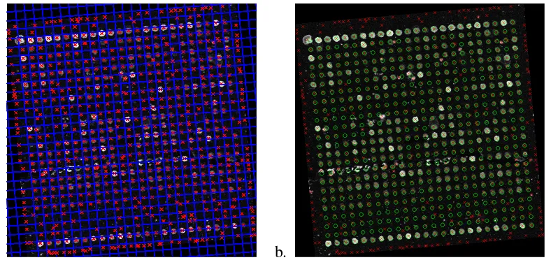
original microarray image using the steps detailed in Section 2.5. Figure 6b. shows the final result, after matching the ideal spot centres of the template to the observed spot centres. Green circles indicate the position corresponding to the estimated template. Note also how spurious spot centres corresponding to noise and image artifacts have been discarded.

a. b.

Figure 6: a. Separating lines delimiting texture primitives (spots). b. Template spots overlapped on the observed subgrid image (red crosses indicate observed spot centres and green circles are template spots.

The whole procedure was applied to different real microarray images from the dataset of Alizadeh

et al.[1]. This dataset also provides the addressing results obtained by processing them with the semi-automatic software tool ScanAlyze 2.3 [11]. The Root Mean Square Error (RMSE) was computed between the estimated spot centres addressed using the automatic method proposed in this work and the true spot centres calculated with ScanAnalyze. It is noticeable that as ScanAlyze is a semiauto-matic tool, there may be mistakes introduced by user selection. The results are reported in Table 1.

Table 1: RMSE (in pixels) between the estimated location of the spot centres using the proposed automatic method and the positions obtained with the semiautomatic tool ScanAlyze.

Image ID Number of spots RMSE inx RMSE iny Total RMSE

lc8n015rex2 18432 3.43 8.35 9.03

lc7b104rex2 9216 3.49 3.85 5.20

lc7b023rex2 9216 3.42 3.77 5.09

lc7b017rex2 9216 3.77 4.73 6.05

lc7b046rex2 9216 3.34 4.08 5.27

lc4b063rex2 9216 5.75 4.98 7.61

4

CONCLUSIONS AND FUTURE WORK

In this paper an automatic approach is proposed to address the location of microarray subgrid spot centres. It relies on the assumption that spotted microarray images can be regarded as texture images and consequently texture analysis techniques are suitable to be applied. This is because of the regularity and pseudo-periodicity exhibited by microarray images.

The present approach computes the displacement vectors that span the spot lattice, finding with a single technique the image angle of rotation and the row and column spot spacing. These ap-proach is based on the computation of the generalized Hough transform with the candidate peaks ordered according to their region of dominance in the autocorrelation function. Instead of using the raw autocorrelation image, this image is previously segmented by means of morphological binary operations and connected components detection. The centres of these components are computed to get continuous coordinates for the peaks and consequently, continuous cartesian components for the displacement vectors.

A grid template is generated from the two displacement vectors and then it is matched to the original spot centres. The RMSE was calculated between the estimated spot locations and the ones obtained by the semiautomatic tool ScanAnalyze in order to evaluate the performance of the proce-dure. The method yields promising results. However, a refinement procedure would be desirable to reduce the estimation error improving accuracy. This procedure is currently under development.

REFERENCES

[1] Alizadeh A. A., Eisen M. B.,et al. Distinct types of diffuse large B-cell lymphoma identified by gene expression profiling. Nature, 403(6769):503–511, February 2000.

[2] Angulo J. and Serra J. Automatic analysis of DNA microarray images using mathematical morphology. Bioinformatics, 19(5):553–562, 2003.

[3] Attwood T. K. and Parry-Smith D. J. Introduction to bioinformatics. Addison Wesley Longman Limited, Harlow, England, 1999.

[4] Bajcsy P. Gridline: Automatic grid alignment in DNA microarray scans. IEEE Transactions on Image Processing, 13(1):15–25, 2004.

[5] Bajcsy P. An overview of DNA microarray grid alignment and foreground separation ap-proaches. EURASIP Journal on Applied Signal Processing, Article ID 80163:1–13, 2006.

[6] Berrar D. P., Dubitzky W., and Granzow M., editors. A practical approach to microarray data analysis. Kluwer Academic Publishers, Dordrecht, 2003.

[7] Blekas K., Galatsanos N. P., Likas A., and Lagaris I. E. Mixture model analysis of DNA microarray images. IEEE Transactions on Medical Imaging, 24(7):901–909, 2005.

[8] Carstensen J. M. An active lattice model in a Bayesian framework. Computer Vision and Image Understanding, 63(2):380–387, 1996.

[9] Ceccarelli M. and Antoniol G. A deformable grid-matching approach for microarray images.

[10] Demirkaya O., Asyali M. H., Shoukri M. M., and Abu-Khabar K. S. Segmentation of microar-ray cDNA spots using MRF-based method. the 25th Annual Conference of the IEEE EMBS, Cancun, Mexico, 2003.

[11] Eisen M. Scanalyze. 1999. http://rana.lbl.gov/EisenSoftware.html.

[12] Gonzalez R. and Woods R. Digital image processing. Prentice Hall, 2nd. edition, 2002.

[13] Gonzalez R. C., Woods R. E., and Eddins S. L. Digital image processing using MATLAB. Prentice Hall, 2004.

[14] Hartelius K. and Carstensen J. M. Bayesian grid matching. IEEE Transactions on Pattern Analysis and Machine Intelligence, 25(2):162–173, 2003.

[15] Heyer L. J., Moskowitz D. Z., Abele J. A., Karnik P., Choi D., Malcolm Campbell A., Old-ham E. E., and Akin B. K. MAGIC tool: integrated microarray data analysis. Bioinformatics, 21(9):2114–2115, 2005.

[16] Hirata Jr. R., Barrera J., Hashimoto R. F., and Dantas D. O. Microarray gridding by mathemati-cal morphology. InProc. SIBGRAPI, Florian ´opolis, pages 112–119. IEEE, 2001.

[17] Hirata Jr. R., Barrera J., Hashimoto R. F., Dantas D. O., and Esteves G. H. Segmentation of microarray images by mathematical morphology. Real-Time Imaging, 8:491–505, 2002.

[18] Jin H.-J., Chun B.-K., and Cho H.-G. Extendedδ-regular sequence for automated analysis of microarray images. EURASIP Journal on Applied Signal Processing, Article ID 13623:1–11, 2006.

[19] Katzer M., Kummert F., and Sagerer G. Methods for automatic microarray image segmentation.

IEEE Transactions on Nano-Bioscience, 2(4):202–214, 2003.

[20] Li Q., Fraley C., Eugene Bumgarner R., Yeung K. Y., and Raftery A. E. Donuts, scratches and blanks: robust model-based segmentation of microarray images. Bioinformatics, 21(12):2875– 2882, 2005.

[21] Li S. Z. Markov Random Field modeling in computer vision. Springer-Verlag, 1995.

[22] Lin H.-C., Wang L.-L., and Yang S.-N. Extracting periodicity of a regular texture based on autocorrelation functions. Pattern Recognition Letters, 18:433–443, 1997.

[23] Liu Y., Collins R. T., and Tsin Y. A computational model for periodic pattern perception based on frieze and wallpaper groups. IEEE Transactions on Pattern Analysis and Machine Intelligence, 26(3):354–371, 2004.

[24] Schena M., Shalon D., Davis R. W., and Brown P O. Quantitative monitoring of gene expression patterns with a complementary cDNA microarray. Science, 270:467–470, 1995.

[25] Yang Y., Buckley M., Dudoit S., and Speed T. Comparison of methods for im-age analysis on cDNA microarray data. Technical Report #584, Department of Statis-tics, University of California, Berkeley, November 2000. Document available at URL: http://www.stat.berkeley.edu/users/terry/zarray/TechReport/584.pdf.