A solution to the materialized view selection problem in data warehousing

A Solution to the Materialized

View Selection Problem in Data

Warehousing

Ayelen S.Tamiozzo1*, Juan M. Ale 1,2

1

Facultad de Ingenieria, Universidad de Buenos Aires, 2 Universidad Austral

Abstract. One of the most important decisions in the physical designing of a data warehouse is the selection of materialized views and indexes to be created. The problem is to select an appropriate set of views and indexes to storage that minimizes the total query response time, as long as the cost of maintaining them, given a constraint of some resource like storage space, is kept as low as possible.

In this work, we have developed a new algorithm for the general problem of se-lection of views considering indexes, as an extension to a well-known algorithm . We present a heuristic for selection of views and indexes to optimize total que-ry response under a materialization time constraint. Finally, we present an ex-perimental comparison of our proposal with the considered state-of-art ap-proach.

Keywords: Views, View Selection, Data Warehouse, Indexes, Materialization

1

Introduction

On-line analytical processing (OLAP) and data warehousing are essential elements of decision support systems (DSS), which are aimed at enabling managers to make better and faster decisions. DSS have become a key to obtain competitive advantages for business. Business analysts want to run decision support applications to detect busi-ness trends by mining the data stored in the information sources. Typically, the infor-mation sources do not maintain historical data but this data is stored in the data ware-house, causing that the data warehouse database tends to be very large and grow over time. Also, the decision support applications run very complex queries over these information sources. Because of this, the queries tend to take unacceptably long to complete. To reduce this time, there are special purpose query optimization and in-dexing techniques. Another commonly used technique is to precompute frequently

asked queries and store them in a data warehouse. They are known as materialized views

The prominent role of materialized views and indexes in improving query-processing performance has long been recognized, see, for instance, [1], [2]. Typical-ly, strategies were developed to improve query evaluation costs to some degree, by using, for instance, greedy algorithms for choosing indexes or views. However, it is nontrivial to arrive at a globally optimum solution, one that reduces the processing cost of typical OLAP queries as much as is theoretically possible.

As we show in our experiments, our proposal results in high-quality solutions - in fact, in globally optimum solutions for many realistic-size problem instances. Thus, they compare favorably with the well-known AND-OR View Graph-centered ap-proach of [2].

We can talk about "globally optimum" solutions only when we have formally de-fined the OLAP view- and index-selection problem. We begin by giving here an in-formal discussion of this optimization problem. We provide a detailed discussion on this topic below. A precise definition of the OLAP view- and index-selection problem is available in [3].

In our OLAP view- and index-selection problem, (1) the inputs include the data-warehouse schema, a set of data-analysis queries of interest and a maintenance cost constraint, and (2) the output is a set of definitions of those views and indexes that minimizes the cost measure for the input queries, subject to the input constraint. For each instance of this optimization problem one can find a globally optimum solution, for instance by complete enumeration of all potential solutions. For realistic-size problem instances, the size of this search space tends to be very large, thus finding optimum solutions is infeasible by brute-force methods. In fact, NP-completeness of a variant of the problem described here is proved in [1].

In this paper an efficient heuristic algorithm for the view- and index-selection problem under the maintenance time constraint is proposed. We address this problem in general AND-OR view graphs using an A* logic to arrive at a possible optimal solution.

The rest of the paper is organized as follows. We review related work in Section 2. In section 3 we discuss the formulation and settings for our OLAP view- and index-selection optimization problem, and present our propose approaches. In section 4, we present and discuss our experimental results. We conclude in section 5.

2

Related Work

Indexing technique has been used extensively in order to facilitate and optimize query processing. The research on index generation and access path selection has been ex-tensively studied from earlier day in 1970s to now [1], [4], [5], [6].

when there are only queries with aggregates over the base relation. The view graphs that arise in OLAP applications are special cases of OR view graphs. The authors in [7] provide a polynomial-time greedy algorithm that delivers a near-optimal solution. Gupta at al. in [1] extend their results to selection of views and indexes in data cubes. Gupta in [2] present a theoretical formulation of the general view-selection problem in a data warehouse under space or maintenance time constraint and generalizes the previous results to: (i) OR view graph with and without indexes, (ii)AND view graph with and without indexes, (iii) AND OR view graph without taking into account in-dexes, (iv) OR view graph under time constraint and (v) AND OR view graph under time constraint (i, ii and iii are just under space constraint). Even thoughT most of the work considered the space as a constraint, in practice is less applicable, because disk space is very cheap in real life. The real constraining factor that prevents us from materializing everything at the warehouse is the maintenance time incurred in keeping the materialized views up to date.

There are several papers that summarize the state of art, just as [8], [9], [10] where there are summarize the different view selection methods with their classifications, like:

 Algorithm type: deterministic randomized, hybrid, etc

 Resource constraint: typically space [11], but also maintenance cost con-strained [12]

 Frameworks: how to identifies the candidate views, just like multiquery DAG, syntactical analysis of the workload [13] [14] or query rewriting.

At our knowledge, the present article is the first to address the problem of selecting views to materialize and indexes to create in a data warehouse under the constraint of a given amount of total maintenance time.

3

View Selection in AND OR View Graphs

In this section, we present definitions and notation from [2] to be used in this article. Furthermore, we recall the well-known A * algorithm from [7]

3.1 Notation and definitions

We use V(G), and E(G) to denote the set of vertices and edges respectively of a graph G.

Expression ANDOR-DAG: An expression ANDOR-DAG for a view or a query V is a directed acyclic graph with V as a source and the base relations as sinks. Each non-sink node v has associated with it one or mode AND arcs, where each AND arc binds a subset of the outgoing edges of node v. As in the previous definition, each AND arc has an operator and a cost associated with it. More than one AND arc at a node de-picts multiple ways of computing that node.

AND-OR View Graph: A directed acyclic graph G having the base relations as the sinks is called an AND-OR view graph for the views (or queries) if for each , there is a subgraph in the G that is an expression ANDOR-DAG for Each node v in an AND-OR view graph has the following parameters associated with it: query-frequency (frequency updates on v), update frequency (frequency of updates on v), and reading cost (cost incurred in reading the materialized view v). Also, there is a maintenance-cost function UC (update cost) associated with G, such that for a view v and a set of views M, UC(v,M) gives the cost of maintaining v in presence of the set M of materialized views.

Given a set of queries to be supported at a warehouse, [15] shows how to construct an AND-OR view graph for the queries.

The maintenance-cost view and index selection problem consist in select a set of views and indexes in order to minimize the total query response time under a given maintenance-cost constraint. Given an AND-OR view graph G and a quantity S (available maintenance time), the problem is to select a set of views and indexes M, a subset of the nodes in G, that minimizes the total query response time such that the total maintenance time of the set M is less than S.

More formally, let Q(v,M) denote the cost of answering a query v (also a node of G) in the presence of a set M of materialized views and indexes. As defined before, UC(v,M) is the cost of maintaining a materialized view or index v in presence of a set M of materialized views and indexes. Given an AND-OR view graph G and a quanti-ty S, the maintenance-cost view-selection problem is to select a set of views/nodes M, that minimizes , where

(1)

under the constraint that U(M)≤S, where U(M), the total maintenance time, is defined as

(2)

In [16] is shown how to compute the cost of answering a query v in presence of M (Q(v,M)) and the maintenance cost of a view v with respect to a selected set of mate-rialized views M (UC(v,m)).

the minimum set cover problem. It is trivial to see that considering also the indexes on the logic keeps this property, as the indexes can be considered in the ANDOR view graph in the same way that the views (just nodes).

A property that makes more complex to solve a maintenance-cost view-selection problem than the space constraint problem is the non-monotonic property. In the case of the space-constraint problem, as the query benefits of a view never increases with materialization of other views, the query-benefit per unit space of a non-selected view always decreases monotonically with the selection of other views. This property is formally defined in [15] as the monotonicity property of the benefit function:

Monotonicity Property: A benefit function B, which is used to prioritize views for selection, is said to satisfy the monotonicity property for a set of views M with respect to distinct views if is less than (or equal to) either or if .

3.2 The A* Algorithm

we present an A* heuristic that, given an AND-OR view graph and a quantity S, deliver a set of views M that has an optimal query response time such that the total maintenance cost of M is less than S. An A* algorithm [17] searches for an optimal solution in a search graph where each node represents a candidate solution. Roussopoulos in [18] also demonstrated the use of the A* heuristics for selection of indexes in relational databases. .

We describe the A* heuristic used to obtain an optimal solution from the views to materialize with S as total maintenance constraint.

Algorithm 1: A* heuristic

1.Create a search graph, G, consisting solely of the start

node, n0. Put n0 on a list called OPEN.

2.Create two list called CLOSED and VISITED that are

initial-ly empty. Set U (accumulate update cost) as 0.

3.If OPEN is empty, exit successfully with the solution

ob-tained by creating a graph with the nodes on CLOSED.

4.Select the first node (n) on OPEN (order by minimal f(x)),

remove it from OPEN, and put it on VISITED.

5.If [(UC(n) + U) > S] go to 3.

6.Put n in CLOSED. U += U + UC(n)

7.For each node successor from n, if they are not already on

VISITED, add them to OPEN. Otherwise, redirect its pointer parent to n if the best path to m found so far is through n.

8.Go to 3.

3.3 AND OR View Graph with Indexes

Here we describe how we used a procedure based on the A* algorithm to solve the view-index selection problem.

First of all, we describe how to obtain the input of the algorithm. We followed the systematic way of obtaining the AND-OR view graph explained on [18], with some modifications:

a. obtain the query model

b. integrate the queries into an AND-OR DAG

c. integrate the AND-OR DAG into a AND-OR View graph d. obtain the update probabilities of the views and indexes e. obtain the sizes of the views and indexes

The idea is the following: we obtain all the queries and updates which will be used into the optimization process, for example based on the history of use of the database. Having obtained the query model, it is processed to obtain an AND-OR DAG as it is explained in [19], where the nodes of the graphs represent either indexes or views, that the later were created from the parents by applying one of the following opera-tors: horizontal selector, vertical selector, join, union or intersection. From each query used, we obtain an AND-OR Dag.

On the next step, all the AND-OR Dags are processed to obtain just an AND-OR View graph, that consist in recognize the nodes from different Dags that are actually semantically equal or that can be connected through one of the operators mentioned above.

The last two steps are estimated according to [18] for indexes and following the guidelines of [16] for views.

Once we have the input, we should compute the function f(x), used in step 4. f(x) results from adding g(x) and h(x)):

g(x) is the total query cost of the queries V(G) using the selected views in M f ,M (3)

h(x) is an estimated lower bound on h*(x) which is defined as the remaining query cost of an optimal solution corresponding so tome descendant of x in G. In other words, h(x) is the actual cost of the minimal cost path between node x and a goal node. . We use ideas from both [8] and [6] in our heuristic to compute this function, depending on if we were working with a index node or a view node.

The following theorem proved in [7] provides

Theorem 1: the A* heuristic returns an optimal solution if: 1. Each node in the graph has a finite number of successors 2. All arcs in the graph have a cost than some positive amount e

3. For all nodes n in the search graph, h*≤h. That is, h* ne er o erestimates the actual value, h

from it and is always a finite number. The second condition is also succeeding, as the cost of the nodes is the update time cost and it is always a positive amount.

On [16], the authors prove that for the view selection problem, the third condition is met. For the other hand, on [18] the same is proven for indexes. Considering both demonstrations, we can conclude that the presented heuristic is also optimal.

In the worst case, the A* heuristic can take exponential time in the number of nodes in the view graph.

4

Performance Evaluation

We run some experiments to determine the quality of the solution delivered and the time taken in practice by the A* heuristic. To perform the tests, we use the database published in †, where we could work with tables from some Megabytes each . For the sake of space, we remit the reader to the website where he/she can find the details of the database used in the experimentation. Here is a brief description about the tables being used:

 Comments (215.642 rows)

 Posts (153.081 rows)

 PostHistory (345.077 rows)

 Users (108.245 rows)

 Votes (1.466.687 rows)

We built four different scenarios that all of them, except for the first case, have the same update cost constraint:

1. Tables that do not have any index that can be used in the queries 2. Tables and materialized views, described in [16]

3. Tables and indexes, presented in [18]

4. Tables, indexes and materialized views, defined in this paper.

In all cases, we use an implementation of the A* heuristic to select the indexes or materialized views to create. We used a linear cost model [2] for the purposes of our experiments.

We run the same set of queries for the four scenarios and measure how much time takes to resolve all of them:

Q1- select users.id from users,posts where posts.OwnerUserId

=users.id and posts.PostTypeId=1 union select users.id from us-ers,postshistory,posts where postshistory.userid=users.id and posts.id = postshistory. postid and posts.posttypeid=1;

Q2- select votes.votetypeid,count(posts.id) from votes, posts

where votes.postid = posts.id and posts.PostTypeId = 1 group by votes.votetypeid;

Q3- select users.id from users,comments where

us-ers.id=comments.userid;

Q4- select posts.id, comments.id from posts,comments where posts.id = comments.postid and posts.PostTypeId = 1;

Observations. In light of the performance guarantees (Theorem 1) of the algo-rithm, our experiment arrives to optimal solutions, for the three scenarios where a selection was required.

Regarding the run time of the selection algorithm, the A* heuristics grows expo-nentially in the size of the input graph. However, on considering more structures, the time increases, as the AND-OR view graph gets bigger (for an graph of 30 material-ized views takes about 8 sec but for the same graph considering also indexes, it takes 25 sec).

After running the A* logic, we create the following structures for each scenario: Scenario 2, Materialized views: The logic suggested creating five different views Scenario 3, Just indexes: The heuristic selected six indexes to be created.

Scenario 4, indexes and materialized views: The algorithm suggested four indexes and three materialized views.

Explanation of Figures. The comparison of the time taken by the four scenarios is presented in Figures 1 and 2.

In Figure 1, we show how the time to answer some queries changes if we consider materialized views or not, in scenarios1 and 2, respectively. As we can see, there is a considerable difference in the response time in the first query, mainly due to there are many materialized views that were created to help that query, since it was the one that more time was taking without breaking the update time constraint. Some of these materialized views also helped the second query, but did not resolve it completely, causing that the run time is not so different, and the same happens with the fourth query. Finally, for the third query, none of the created materialized views affect this query. Something quite important to mention is that in no one of queries executed the scenario 2 is slower than the 1. Considering all the queries, the fact of including the materialized views improves the running time in a 76%.

Figure 1: Comparison from Scenario 1 and Scenario 2

0 5000 10000 15000

Q1 Q2 Q3 Q4

R

e

sp

o

ns

e

ti

me

[s]

Query Scenario 1 vs Scenario 2

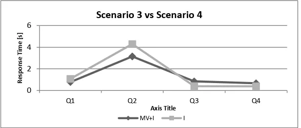
Figure 2: Comparison from Scenario 3 and 4.

In Figure 2, we compare the query response time considering indexes with or without materialized views (scenario 3 and 4). In this case, the time response from both is not significant different.. However, if we take into account all the queries, considering the indexes and materialized views is about 12% faster than just considering indexes, 700 times faster than considering just materialized views and 3000 times quicker than just considering the tables. Something that we would like to mention is that the differ-ence between the scenario 3 and 4 (just indexes against indexes and materialized views) grows if the base tables are bigger or if the partial results have more rows, causing the creation of materialized views more necessary.

5

Conclusions and Future Work

In this paper we undertook a systematic study of the OLAP view- and index-selection problem, and proposed an approach that takes into account both selections under a cost time constraint. Our experiments show that our proposed heuristic to view and index selection result in high-quality solutions. Thus, they compare favorably with the well-known OLAP centered approach [1] for indexes and [16] for materialized views. We have designed our approach to be generic. r. Moreover, we could also extend our approach to other performance techniques, such as buffering, physical clustering or partitioning [20] [21] [22].Finally, the main possible evolution for our work resides in improving our solution's running time, pre-computing the potential indexes-views to minimize the AND-OR View Graph or even working with another heuristics that, keeping an optimal solution, works with in a polynomial time.

6

References

1. Gupta, H., Harinarayan, V., Rajaraman, A., Ullman, J.: Index Selection for OLAP. ACM SIGMOD (1996)

2. Gupta, H., Mumick, I.: Selection of View to Materialize in a Data Warehouse. (2005)

0 2 4 6

Q1 Q2 Q3 Q4

R

e

sp

o

ns

e

T

ime

[s]

Axis Title

Scenario 3 vs Scenario 4

3. Asgharzadeh, Z., Chirkova, R.: Exact and Inexact Methods for Selecting Views and Indexes for OLAP Perfomance Improvement. EDBT (2008) 4. Sun, J.: Index Selection: A Query pattern Mining Based Approach. (2013) 5. Aouiche, K., Darmont, J.: Data Mining-based Materialized View and Index

Selection in Data Warehouses. (2007)

6. Chaudhuri, S.: AutoAdmin "What-if" Index Analysis Utility. In SIGMOD Conference (1998)

7. Ullman, J., Rajaraman, A., Harinarayan, V.: Implementing Data Cubes Efficiently. SIGMOD (1996)

8. Mami, I., Bellahsene, Z.: A Survey of View Selection Methods. SIGMOD (2012)

9. Nalini, T., Kumaravel, A., Rangarajan, K.: A comparative Study analysis of Materialized View for Selection Cost. IJCSES (2012)

10. Thakur, G., Gosain, A.: A Comprehensive Analysis of Materialized Views in a Data Warehouse Environment. IJACSA (2011)

11. Baril, X., Bellahsène: Selection of Materialized Views: a Cost-Based Approach. (2002)

12. Gupta, H., Mumick, I.: Selection of Views to Materialize in a Data Warehouse. (2005)

13. Chaudhuri, S.: Automated Selecion of Materialized Views and Indexes for SQL Databases. 26th International Conference on Very Large Database (2000) 14. Goldstein, J., Larson, P.-A.: Optimizing Queries Using Materialized Views:

A Practical, Scalable Solution. ACM SIGMOD 2001 (2001)

15. Gupta, H.: Selection of views to materialize in a data warehouse. Proceedings of the Intl. Conf. on Database Theory (1997)

16. Gupta, H., Mumick, I.: Selecction of Views to Materialize Under a Maintenance Cost Constraint. ICDT (1999)

17. Nilsson, N.: Artificial Intelligence - A new Synthesis. Morgan Kaufmann Publishers, Inc. (1998)

18. Roussopoulos, N.: View Indexing in relational databases. ACM Transactions on Database Systems (1982)

19. Roussopoulos, N.: The Logical Access Path Schema of a Database. IEEE Transactions on Software engineering, Vol. SE-8, No. 6 (1986)

20. Agrawal, S., Chaudhuri, S., Kollár, L., Marathe, A., Narasayya, V., Syamala, M.: Database Tuning Advisor for Microsoft SQL Server 2005. VLDB (2004)

21. Bellatreche, L., Boukhalfa, K., Mohania, M.: An evolutionary approach to schema partitioning selection in a data warehouse environmen. DaWaK (2005) 22. Zilio, D., Rao, J., Lightstone, S., Lohman, G., Storm, A., Garcia-Arellano,