Exact solutions for electromagnetic fields inside and outside a spherical
surface with magnetic/electric dipole distributed sources
E. Ley-Koo
Instituto de F´ısica, Universidad Nacional Aut´onoma de M´exico, Apartado Postal 20-364, 01000 Ciudad de M´exico, M´exico.
Ch. Esparza-L´opez
Department of Applied Mathematics and Theoretical Physics, Center for Mathematical Sciences, University of Cambridge, Wilberforce Road, Cambridge CB3 0WA, UK.
H. Torres-Bustamante
Facultad de Ciencias, Universidad Nacional Aut´onoma de M´exico, Circuito Exterior S/N, 04510, Ciudad de M´exico, M´exico.
Received 13 November 2017; accepted 22 January 2018
Exact solutions of the Maxwell equations for the electromagnetic fields inside and outside a spherical surface, with time alternating magnetic or electric dipole source distributions, are constructed as alternatives to the respective familiar point-dipole solutions in undergraduate and graduate books. These solutions are valid for all positions, inside and outside the sphere, including the quasi-static, induction and radiation zones; the solutions inside make the difference from the point-dipole solutions; the definitions of the dynamic dipole moments must be based on the ordinary spherical Bessel functions for the solutions outside, and on the outgoing spherical Hankel functions for the solutions inside, instead of the powers of the radial coordinate as solutions of the Laplace equation valid for the static case. The solutions for the resonating cavities are associated with the nodes of the spherical Bessel function for the TE modes of the magnetic dipole source, and with the extremes of the product of the radial coordinate times the same spherical function for the TM modes of the electric dipole source; both conditions also guarantee the vanishing of the fields outside.
Keywords: Time alternating electric and magnetic dipole sources; potentials and force fields; inner and outer exact solutions; Helmholtz equation; boundary condition forms of Maxwell equations; outgoing-wave Green function multipole expansion.
PACS: 41.20.Jb.
1.
Introduction
The introductory examples of electromagnetic radiation, in the advanced undergraduate and graduate levels, are com-monly those of the Hertz electric and magnetic point-dipole sources with a harmonic time variation; in addition the study of the electromagnetic radiation in resonant cavities is pre-sented separately [1-11]. Our experience with the multipole expansions of the electrostatic and magnetostatic fields [12], and of the electromagnetic fields [13] and of their respec-tive sources distributed on a spherical surface, shows the ex-istence of complete and exact solutions inside and outside such a boundary surface, for each multipole component. In this contribution, we construct the electromagnetic radiation solutions for the finite electric and magnetic dipole sources, applicable for both antennas and resonant cavity modes.
In Sec. 2, the magnetic dipole case is analyzed first be-cause it is didactically simpler. In fact, it involves a surface current with a sine of the polar angle distribution along par-allel circles. Then, the vector potential and the electric inten-sity inherit the alternating time variation, the dipolarity and parallel-circle field lines of their source; additionally, they share the same radial dependence in terms of spherical Bessel functions of order 1 : ordinary ones inside and of Hankel type outside, and with coefficients involving the other function at the radius of the boundary surface guaranteeing their continu-ity there. The magnetic induction field is evaluated as the
ro-tational of the vector potential, with radial components con-tinuous at the boundary surface, and polar angle tangential components with a discontinuity connected with the source current by Ampere’s law.
the dynamical dipole moments, involving the coefficients in the other spherical Bessel function, for the fields inside and outside. The characterization of the transverse electric TE and magnetic TM modes, of the respective resonant cavities, depends on the boundary conditions on the inner solutions, which at the same time guarantee the vanishing of the fields outside.
Section 4 includes a discussion of the results for the mag-netic dipole and the electric dipole fields, a comparison of their similarities and differences, as well as their complemen-tarities; and the formulation of some didactic comments.
2.
Magnetic Dipole Sources, Potential and
Fields
The linear current density distribution on parallel circles on the spherical surface has the form:
~
K= ˆϕK0sinθe−iωt
= (−ˆısinϕ+ ˆcosϕ)K0sinθe−iωt, (1)
which in its cartesian representation exhibits its harmonic dipole components. Since its divergence vanishes, the con-tinuity equation indicates that there is not a companion dis-tribution of charge.
The vector electromagnetic potential shares the same time and multipolarity dependences of its source, as well as the radial spherical Bessel functions inside and outside of the sphere as solutions of the Helmholtz equation [14]:
~
A(r≤a, θ, ϕ, t) = ˆϕA0ij1(kr) sinθe−iωt (2)
~
A(r≥a, θ, ϕ, t) = ˆϕAe
0h (1)
1 (kr) sinθe−iωt (3)
The choices of the ordinary and outgoing spherical wave radial functions guarantee that the boundary conditions for
r → 0 and r → ∞, respectively, are properly satisfied. The condition of continuity of the potential at the spherical boundary becomes:
Ai
0j1(ka) =Ae0h (1)
1 (ka) (4)
making each coefficient proportional to the radial function on the other side
Ai
0=A0h(1)1 (ka), Ae0=A0j1(ka) (5)
c ∂t
= iω
c ϕAˆ 0j1(kr<)h
(1)
1 (kr>) sinθe−iωt, (7) with the explicit forms:
~
E(r≤a, θ, ϕ, t) = iω
c ϕAˆ 0j1(kr)h
(1)
1 (ka) sinθe−iωt (8)
~
E(r≥a, θ, ϕ, t) = iω
c ϕAˆ 0j1(ka)h
(1)
1 (kr) sinθe−iωt (9)
sharing the same space and time dependence, including the multipolarity, direction and solenoidal nature of their com-mon source.
The magnetic induction field is evaluated as the rotational of the potential taking the explicit forms:
~
B(r < a, θ, ϕ, t) =A0h(1)1 (ka)
µ
ˆ
r2 cosθ r j1(kr)
−θˆsinθ r
d
dr[rj1(kr)] 
e−iωt (10)
~
B(r > a, θ, ϕ, t) =A0j1(ka)
µ
ˆ
r2 cosθ
r h
(1) 1 (kr)
−θˆsinθ r
d dr
h
rh(1)1 (kr)i ¶e−iωt. (11)
Notice the continuity of its normal components at the spherical boundary, consistent with Gauss’ law. On the other hand, notice the discontinuity of its tangential polar compo-nents at the same boundary, which by Ampere’s law [11]
ˆ
r׳B~e−B~i´ ¯¯¯
¯
r=a = 4π
c K~ (12)
is connected with the linear density current:
−ϕAˆ 0sinθ
a µ
j1(ka)d
dr h
rh(1)1 (kr)
i
−h(1)1 (ka) d
dr[rj1(kr)] ¶¯¯
¯ ¯ ¯
r=a
e−iωt
=−ϕAˆ 0 i
ka2sinθe
−iωt= ˆϕ4π
c K0sinθe
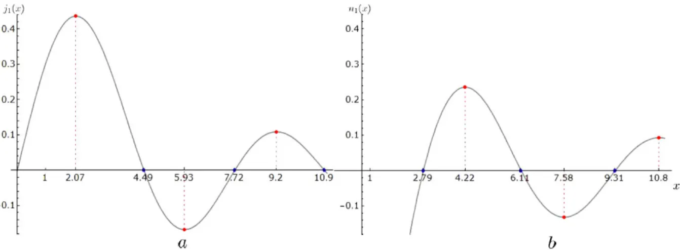
FIGURE1. Plot of the real and imaginary parts of the spherical Hankel function:j1(ka)andn1(ka), respectively, singularazing their lowest
roots:x1,sandy1,s, identifying the nodal lines, including the resonant cavity modes, and the positions of their extreme values: xext1,s and yext
1,s, optimizing the radiation by antennas.
The quantity inside the parenthesis in the first line is identi-fied askatimes the Wronskian of the spherical Bessel func-tions: i/k2a2. The result of the next line yields the
relation-ship between the amplitudes of the vector potential and the current distribution:
A0= 4πika2K0. (14)
The current Eq. (1), the vector potential Eq. (6) and the electric intensity field Eq. (7) all share parallel circle field lines. The field linesd~l= ˆrdr+ ˆθrdθ for the magnetic in-duction field inside and outside Eqs. (10) and (11), can also be evaluated from the tangentiality conditions:
dr
2j1(kr) cosθ =
rdθ
−sinθdrd [rj1(kr)]
, (15)
dr
2h(1)1 (kr) cosθ
= rdθ
−sinθd dr
h
rh(1)1 (kr)i. (16) Both equations are separable and integrable, leading to the equations for the lines passing by a point (r0, θ0), in any
meridian plane:
h(1)1 (ka)krj1(kr) sin2θ=h(1)1 (ka)kr0j1(kr0)
×sin2θ0 r0< a , (17)
j1(ka)krh(1)1 (kr) sin2θ=j1(ka)kr0h(1)1 (kr0)
×sin2θ
0 r0> a . (18)
Here the inclusion of the coefficient of the other spherical Bessel function in each of these equations, coming from Eq. (6), allows also the direct comparison of the field lines inside and outside the spherical surface: continuous in the contributions from the real parts, and discontinuous in the contributions from the imaginary parts associated with the Wronskian in Eq. (13).
Figure 1 displays the coefficients in Eqs. (17)-(18) as the real and imaginary parts of the Hankel function: j1(ka)and
n1(ka), respectively. The roots of the first function: x1,s = 4.49,7.72,10.9...determine the nodal circle lines inside the boundary surface, and those ofn1:y1,s= 2.79,6.11,9.31... determine the nodal circle lines outside. The extremes ofj1
determine the optimal amplitude for the external fields. Figures 2 a,b,c illustrate magnetic induction field lines of Eqs.(10) and (11) in their forms of Eqs.(17) and (18), in-side and outin-side the spherical surface in black, on any merid-ian plane at a given instant of time. The alternating lines in red and blue are closed, exhibiting their solenoidal character, and have opposite circulation directions; their separatrices in green dashed circles indicate the vanishing of the field there. Notice also the discontinuities of the field lines at the spheri-cal surface where the current is distributed, Eq.(12).
On the other hand, the conditions for the transverse elec-tric TE modes of the cavity with vanishing radial and polar components of the electric intensity can be appreciated in Eq. (8), and the vanishing of the normal component of the magnetic induction at the source boundary: j1(ka) = 0 in
Eq.(10) leads to the choices of the nodes from Fig. 1. The appearance of this common coefficient in the external elec-tric intensity field, Eq. (9), and in the external magnetic in-duction field, Eq. (11), leads to the vanishing of the elec-tromagnetic fields everywhere outside. Figures 3 a,b,c il-lustrate the magnetic induction field lines in the lower TE modes of the resonant cavity for the respective frequencies:
ω = (4.48724, 7.71886,10.9005), in units of (c/a). The fields along the axis of the cavity also vanish.
FIGURE2. Magnetic induction field lines inside and outside the source spherical surface on black, in any meridian plane and at a given time, for the choices of(a)ka= 1,(b)ka= 2.0710and(c)ka= 5.9280.
FIGURE3. Magnetic induction field lines inside the spherical surface, in any meridian plane and at a given time, for the resonant TE cavity modes for(a)ka= 4.48724,(b)ka= 7.71886and(c)ka= 10.9005.
It is very important to recognize that the results obtained so far are exact. Then, we analyze successively the quasi-static limit and the radiation limit. In fact, for the first one when kr ¿ 1, the ordinary spherical Bessel function be-comes linear and the spherical Hankel function is inversely proportional to the square of the radial coordinate:kr/3and
−i/k2r2, respectively. Then, the magnetic induction field
in-side, Eq. (10), becomes
~
B(r < a, θ, ϕ) =−A0 i
k2a2
2k
3
³
ˆ
rcosθ−θˆsinθ ´
= 4πK0
3 2ˆk, (19)
where the connection between the amplitudesA0andK0has
been used from Eq. (14), and identifying the unit axial vector ˆ
k; in conclusion, the magnetic induction field inside is ax-ial and uniform. Notice that in Fig. 2a) the field inside the sphere is no longer uniform, even forka= 1, and outside is contained by the first node in Fig. 1b).
The field outside, Eq. (11), takes the following form:
~
B(r > a, θ, ϕ) =−A0
µ ia
3k 
ˆ
r2 cosθ+ ˆθsinθ r3
= 4πK0 3
a3
r3
³
3ˆr(ˆr·kˆ)−ˆk´, (20) in which the angular distribution of an axial dipole moment and its inverse cube radial dependence are identified. The respective static magnetic dipole moments determining the fields inside and outside are4πK0/3and4πK0a3/3,
consis-tent with the amplitudes in Eqs. (19)-(20).
It is convenient to point out the different radial depen-dences of the coefficients in Eqs. (19) and (20): independent of the radiusaand with the cube ofa, respectively, reflecting the ratio between the inner and outer dipolar radial depen-dences in the solutions for the Laplace equationrvs1/r2.
On the other hand, in the far away zone wherekrÀ1,
h(1)1 (kr)→ −
eikr
kr , d dr
h
h(1)1 (kr)
i
→ −ike
ikr
then, the radial contribution to the field in Eq. (11) and the term in the derivative ofrin the polar angle direction vanish sooner than the surviving term in the radiation zone:
~
B(r > a, θ, ϕ, t) =−A0j1(ka)ˆθsinθ
d dr
h
h(1)1 (kr)i
×e−iωt→ −4πK0θˆsinθka2j1(ka)
ei(kr−ωt)
r . (22)
Its companion electric intensity field from Eq.(9) be-comes:
~
E(r > a, θ, ϕ, t) =ikϕˆsinθA0j1(ka)h(1)1 (kr)
×e−iωt→4πK
0ϕˆsinθka2j1(ka)e
i(kr−ωt)
r . (23)
These are the exact results for the radiation fields from the sources distributed on the spherical surface, with a common amplitude determined by the value ofj1(ka)there, the same
phase, perpendicularE~ andB~ fields, with a vector product in the radial direction ϕˆ×(−θˆ) = ˆr with asin2θ angu-lar distribution, and a poangu-larization in the ϕˆ direction, per-pendicular to the meridian plane. Now, we can take again the point source limit, arriving at the common amplitude 4πK0a3k2/3 =µk2, using the respective value of the point
static dipole moment and connecting with the familiar re-sults in the books [1-11], including the square dependence on the wave number. At the same time the dynamic magnetic dipole moment can be identified as 4πK0a2j1(ka)/k,
con-sistent with its own dimensions, with the exact amplitudes in Eqs. (22)-(23), and with the point-dipole source limit.
3.
Electric Dipole Sources and Fields
This section involves electric dipole distributions of surface charge density and linear current density along meridian half-circles on the spherical surface:
σ=σ0cosθe−iωt, (24)
~
K=K0θˆsinθe−iωt. (25)
Both densities are connected by the continuity equation
∇ ·K~ +∂σ
∂t = 0, (26)
which allows to obtain the relationship between their respec-tive amplitudes:
K02 cosθ
a −iωσ0cosθ= 0 ∴ K0=
iωσ0a
2 (27)
and to convince the reader about their respective polar angle dependences.
Instead of constructing the scalar and vector potentials, we choose to construct the force fields from their inhomoge-neous Helmholtz equation [11]:
¡
∇2+k2¢B~(~r, t) =−4π
c ∇ ×J~(~r, t), (28)
¡
∇2+k2¢E~(~r, t) =4π
c µ
∇ρ(~r, t) +1
c
∂J(~r, t)
∂t 
, (29)
whereJ~=Kδ~ (r−a)andρ=σδ(r−a). We construct the solution for the magnetic induction field first, Eq. (28), by using the multipole expansion of the outgoing-wave Green function [13]:
G+(~r, ~r0) =eik|~r−~r 0|
|~r−~r0| =ik
X
l
(2l+ 1)
×Pl(ˆr·ˆr0)jl(kr<)h(1)l (kr>) (30)
~
B(~r, t) =1
c Z
∇0×J~(~r0, t)G+(~r, ~r0)d3r0, (31)
where its transverse source is the rotational of the current density, whose explicit form follows from Eq. (25):
∇ ×J~= ˆϕK0sinθ r
d
dr[rδ(r−a)]. (32)
For the dipole source of Eq. (32), only the terml = 1in the sum of Eq. (30) is needed, thus
~
B(~r, t) =ik3K0
c e
−iωt ∞
Z
0
r0 d
dr0 [r
0δ(r0−a)]
×j1(kr<)h(1)1 (kr>)dr0 π
Z
0 2π
Z
0
ˆ
ϕ0sin2θ0
×[sinθsinθ0cosϕcosϕ0+ sinθsinθ0sinϕsinϕ0
+ cosθcosθ0]dθ0dϕ0. (33) The unit vector in its cartesian components ϕˆ0 =
−ˆısinϕ0 + ˆcosϕ0 projects the first and second terms in the square brackets, representing rˆ · rˆ0, when the integration over ϕ0 is performed with explicit result
πsinθsinθ0[ˆcosϕ−ıˆsinϕ] =πsinθsinθ0ϕˆ. This shows that the magnetic induction field is in the direction of parallel circles inherited from its source in Eq. (32). Correspond-ingly, the integration over the third term in the square brack-ets vanishes. Next the integration overθ0,
π
Z
0
sin2θ0sinθsinθ0dθ0
= sinθ
1
Z
−1
(1−η2)dη= 4
3sinθ (34)
The first term vanishes because the Dirac delta function vanishes in both limits. Then the results inside and outside the source spherical surface become, respectively:
~
B(r < a, θ, ϕ, t) =−ϕˆ4πi
c K0sinθ(ka)j1(kr)
×
µ d d(ka)
h
(ka)h(1)1 (ka)
i¶ e−iωt
(36)
~
B(r > a, θ, ϕ, t) =−ϕˆ4πi
c K0sinθ(ka)
×
µ d
d(ka)[(ka)j1(ka)]
h(1)1 (kr)e−iωt (37)
The magnetic induction field shows a discontinuity in its par-allel circle components at the source spherical surface
ˆ
r×
³ ~
Be−B~i´ ¯¯¯
¯
r=a =4π
c K ,~ (38)
according to Ampere’s law [11], measuring the magnitude of the meridian current distribution:
ˆ
θ4πika
c K0sinθ µ
d
d(ka)[(ka)j1(ka)]h
(1) 1 (kr)
−j1(kr) d
d(ka)
h
(ka)h(1)1 (ka)i ¶¯¯¯¯ r=a
= ˆθ4πika
c K0sinθ
−ika k2a2 =
4π
c θKˆ 0sinθ , (39)
where the term inside the parenthesis is identified askatimes the negative of the Wronskian of the spherical Bessel func-tions:−i/k2a2.
While the solution for the electric intensity field could be constructed from its sources, being the gradient of the charge density and the time derivative of the current distribution in Eq. (29), as we already did for the magnetic induction field, it is more expedient to use the Maxwell connection between both fields:
1
c ∂ ~E
∂t =∇ ×B ,~ (40)
−θˆsinθ r
d
d(kr) (kr)h
(1) 1 (kr)
× d
d(ka)[(ka)j1(ka)]e
−iωt. (42)
Notice the continuity of its tangential meridian compo-nents at the spherical boundary, as required by Faraday’s law. On the other hand, notice the discontinuity of its radial com-ponents at the same boundary in agreement with Gauss’ law:
ˆ
r·
³ ~ Ee−E~i
´¯¯ ¯
r=a= 4πK0
ω
2 cosθ r (ka)
×
µ d
d(ka)[(ka)j1(ka)]h
(1) 1 (kr)
−j1(kr)
d d(ka)
h
(ka)h(1)1 (ka)
i ¶¯¯ ¯ ¯
r=a
= 4π2K0ka ωa
−ika k2a2 cosθ
= 4π µ
−2i ωaK0
cosθ= 4πσ0cosθ , (43)
leading to the same relationship of Eq. (27) for the ampli-tudesK0andσ0.
The electric field lines inside and outside the spherical boundary are defined by
dr
2j1(kr)cosrθ
= rdθ
−sinθ
r d
dr[rj1(kr)]
, (44)
dr
2h(1)1 (kr)cosθ r
= rdθ
−sinθ
r d dr
h
rh(1)1 (kr)
i, (45)
which coincide with those of Eqs.(15)-(16). They have the same shape as those in Eqs.(17)-(18) but differ in their coef-ficients involving the derivatives of the product of the radial coordinate with the other Bessel function,
d d(ka)
h
(ka)h(1)1 (ka)ikrj1(kr) sin2θ= d
d(ka)
×
h
(ka)h(1)1 (ka)
i
FIGURE 4. Plot of the real and imaginary parts ofkatimes the spherical Hankel function: (ka)j1(ka)and (ka)n1(ka), respectively, singularazing their lowest roots, optimizing the radiation by antennas, and the positions of their extreme values identifying the inner nodal lines and the resonant cavity TM modes; the outer nodal lines are those ofn1(ka), Eq. (47).
FIGURE5. Electric intensity field lines inside and outside the source spherical surface on black, in any meridian plane and at a given time, for the choices of(a)ka= 1,(b)ka= 4.48724and(c)ka= 7.71886.
d
d(ka)[(ka)j1(ka)]krh
(1)
1 (kr) sin2θ=
d d(ka)
×[(ka)j1(ka)]kr0h(1)1 (kr0) sin2θ0 r0> a . (47)
As in the previous section, the inclusion of the coefficient in-volving the other spherical Bessel function in each of these equations allows also the direct comparison of the field lines inside and outside the spherical surface: continuous in the contributions from the real parts, and discontinuous in the contributions from the imaginary parts associated with the Wronskian in Eq. (43).
Figures 5 a,b,c illustrate the electric intensity field lines in the vicinity of the source spherical surface for increasing val-ues ofka= 1,4.48724,7.71886, the last two corresponding to the nodes of Fig. 4a, which optimize the fields outside. The different colors of the lines inside and outside is due to the charge distribution on the spherical boundary, making their radial components discontinuous while their tangential
components are continuous. In Fig. 5a the value ofkais too small and there are no nodal spheres inside. In Fig. 5b and 5c, one and two internal spherical nodes are recognized in green corresponding to extreme values in Fig. 4a. The lines outside have their respective spherical nodes determined by the nodes in Fig. 4b, alternating their directions in between. Notice the field lines leaving or arriving perpendicularly, from or to the source spherical surface, and becoming tangential to the first outer spherical node.
On the other hand, the conditions for the transverse mag-netic TM modes of the cavity with vanishing radial and po-lar components of the magnetic induction can be appreci-ated in Eq.(36), and the vanishing of the tangential polar component of the electric intensity at the source boundary: (d/d(ka)) [kaj1(ka)] = 0 leads to the choices of the
FIGURE6. Electric intensity field lines inside the source spherical surface on black, in any meridian plane and at a given time, for the resonant TM cavity modes:(a)ka= 2.74371,(b)ka= 6.11676and(c)ka= 9.31662.
modes with respective frequencies:ω = (2.74371, 6.11676, 9.31662), in units ofc/a, associated with the extreme values in Fig. 4a with0,1, and 2nodes, respectively. They origi-nate and end perpendicularly, from and to the source spheri-cal surface, consistent with Gauss’s law. In Fig. 6a there are no internal nodes. In Fig. 6b and 6c the lines leaving or arriv-ing from and to the spherical surface also become tangential to the neighbouring inner spherical node; moving farther in, the reader may identify the similarity with the field lines in Figs. 3a and 3b.
We also analyse the quasi-static and radiation limits for the exact results obtained so far. For the first limit,kr ¿1, the electric intensity field inside, Eq. (41), becomes:
~
E(r < a, θ, ϕ) =4πK0
ω (ka) µ
ˆ
r2kcosθ
3 −θˆ 2ksinθ
3
×
µ i k2a2
=−4π
3 σ0ˆk , (48) where the identification between the amplitudesK0andσ0,
Eq. (27), has been used; then, the electric intensity field in-side is axial and uniform. The reader should compare its downward direction with the upward direction of its counter-part of Eq. (19) for the magnetic induction field, for upward pointing electric and magnetic dipoles, respectively. Notice also that, in a similar manner to the magnetic induction in the previous section, in Fig. 5a the electric intensity field inside the source sphere is no longer uniform, even forka= 1, and outside is contained by the first node in Fig. 4b.
The field outside Eq. (42) takes the form:
~
E(r > a, θ, ϕ) = 4πK0
ω
2ka
3
µ
ˆ
r2 cosθ r
µ
−i k2r2
−θˆsinθ r
i k2r2
¶¶
= 4πσ0 3
a3
r3
µ
3ˆr µ
ˆ
r·kˆ 
−ˆk 
, (49) in which the angular distribution of an axial electric dipole moment and its inverse cube radial dependence are identi-fied. The different directions and space dependences of the
field inside and outside, Eqs. (48)-(49), are accompanied also by the difference in their respective static electric dipole mo-ments: 4πσ0/3and4πσ0a3/3, in the same ratio as those in
Eqs. (19)-(20) in Sec. 2.
On the other hand, in the far away radiation zone where
krÀ1the radial contribution to the electric intensity field in Eq. (42) vanishes sooner than the polar-angle direction term:
~
E(r > a, θ, ϕ, t) =−θˆ4πK0 ω (ka)
sinθ r
× d
d(ka)[kaj1(ka)]
d d(kr)
£
−eikr¤e−iωt
=−θˆ2πka2σ0sinθ d
d(ka)[kaj1(ka)]
ei(kr−ωt)
r , (50)
and its companion magnetic induction field outside in this limit from Eq.(37) becomes:
~
B(r > a, θ, ϕ, t) = ˆϕ4πi
c K0sinθ(ka)
× d
d(ka)[kaj1(ka)]e
ikrre−iωt
=−ϕˆ2πka2σ
0sinθ d
d(ka)[kaj1(ka)]
ei(kr−ωt)
r . (51)
These are exact results for the radiation fields, produced by electric dipole sources distributed on the spherical surface, sharing the same amplitude, the same phase, being perpen-dicular to each other, their vector product(−θˆ)×(−ϕˆ) = ˆr
being radial with thesin2θangular distribution, and the po-larization in meridian planes. Their point source limit in-volves the common amplitude4πa3σ
0k2/3 =pk2,
connect-ing also with the familiar results in the books [1-11]. In general, the dynamic electric dipole moment is identified as (4πσ0a2/k)(d/d(ka)) [kaj1(ka)], consistent with the
4.
Discussion
This section contains successively a summary and discussion of the quantitative and illustrative results in Secs. 2 and 3, a comparison of their similarities, differences and comple-mentarities, as well as the formulation of some comments of didactic interest.
In the case of the magnetic dipole source, Eq. (1) de-scribes its current parallel circle field lines and dipolarity on the boundary spherical surface. The corresponding vector po-tential, Eqs. (2)-(6), and electric intensity evaluated as the time derivative of the latter, Eqs. (7)-(9), share the direction and angular dipolarity of the source, as well as the radial de-pendence and the respective coefficients in terms of the spher-ical Bessel functions, ordinary and of Hankel type, inside and outside, respectively; both are continuous at the bound-ary spherical surface. The magnetic induction is evaluated as the rotational of the vector potential, Eqs. (10)-(11), inside and outside, with radial and polar components in each merid-ian plane; their radial components at the spherical bound-ary are continuous, consistent with Gauss’ law; while their polar components show a discontinuity at the same bound-ary, connected with the dipolar current source as required by Ampere’s law, Eqs. (12)-(13), leading to the relationship be-tween the potential and source amplitudes, Eq. (14); the field lines inside and outside are also identified in their differen-tial equation forms, Eqs. (15)-(16) and their integrated forms (17)-(18); they are the bases for Figs. 2a,b,c illustrating their behaviour in the vicinity, inside and outside, of the source spherical surface where the Faraday and Maxwell electro-magnetic inductions come at play. Figures 3 a, b, c corre-spond to the resonant cavity TE modes determined by the boundary condition of the vanishing ofj1(ka), which
guar-antees that the external fields also vanish, Eqs. (9) and (11). On the other hand, the electric dipole source involves both a charge and a meridian half-circle current distributed on the spherical surface, Eqs. (24)-(25), connected via the continuity equation, Eq. (26), leading to the relationship be-tween their respective amplitudes Eq. (27). The magnetic induction field satisfies the Helmholtz equation with the ro-tational of the current distribution as its source Eq. (28); it can be evaluated as the integral of the latter multiplied by the outgoing-wave Green function in its multipole expansion form Eq. (30). The rotational of the current distribution has parallel circle field lines with a sine of the polar angle depen-dence, as the original meridian current distribution; only the dipolar component in the mulipole expansion is selected by the angular integrations, Eqs. (33)-(34), and the magnetic in-duction field inherits the parallel circle field lines and the sine of the polar angle of its source; its radial dependence is that of the ordinary spherical Bessel and Hankel functions, inside and outside, with coefficients coming from the radial integtion as the negative of the derivative of the product of the ra-dial coordinate and the other Bessel function at the radius of the spherical boundary, Eqs. (35)-(37). The tangential com-ponents of the magnetic induction at the spherical boundary
show a discontinuity, which by Ampere’s law Eq. (38) re-produces the original meridian current distribution, Eq. (39). The electric intensity is evaluated as the rotational of the mag-netic induction via their Maxwell connection Eq. (40), with the explicit forms of Eqs. (41)-(42); exhibiting field lines in each meridian plane with a discontinuity in the radial di-rection at the spherical boundary connected with the surface charge distribution by Gauss’ law, Eq. (43), and consistent with the relationship between the charge and current ampli-tudes; the polar angle components are continuous, consistent with Faraday’s law; their field lines turn out to have the same shapes, Eqs. (44)-(45), as those of the magnetic induction for the magnetic dipole source Eqs. (15)-(16), allowing for the difference in their respective coefficients Eqs. (46)-(47) and Eqs. (17)-(18). Figures 5a, b, c illustrate their behaviour in the vicinity, inside and outside, of the source spherical sur-face, where the normal components are discontinuous, for increasing values of the frequency. Figures 6a, b, c illustrate the electric intensity field lines for the TM modes of the reso-nant cavities determined by the vanishing of the derivative of the product of the radial coordinate and the ordinary spheri-cal Bessel function, or the positions of the extremes of such a product, Fig. 4a, guaranteeing also the vanishing of the ex-ternal fields, Eqs. (37) and (42); notice that the field lines end radially at the source spherical surface where the charges are distributed.
1. R.P. Feynman, R.B. Leighton, M.L. Sands. The Feynman Lec-tures on Physics, Vol. 2 (Addison-Wesley, 1963).
2. P.C. Clemow, An Introduction to Electromagnetic Theory (Cambridge University Press, USA, 1973), Chapter 5.
3. J.R. Reitz, F.J. Milford, Foundations of Electromagnetic The-ory, 3rd ed. (Addison-Wesley, Reading, Mass, USA, 1979), Chapter 20.
4. M.A. Heald, J.B. Marion, Classical Electromagnetic Radiation (Academic Press, New York, USA, 1980), Chapter 8.
5. R.K. Wangsness, Electromagnetic Fields (John Wiley and Sons, New York, USA, 1986), Chapter 28.
6. P.Lorrain, D.R. Corson, Electromagnetic Fields (W.H. Freeman and Co, San Francisco, USA, 1988), Chapter 38.
7. J.Vanderlinde, Classical Electromagnetic Theory (John Wiley and Sons, New York, USA, 1993), Chapter 10.
8. D.J. Griffiths, Introduction to Electrodynamics. 4th ed. (Pear-son, USA, 2013), Chapter 11.
9. W. Greiner, Classical Electrodynamics (Springer-Verlag, New York, USA, 1998), Chapter 21.
10. W.K.H. Panofsky, M. Phillips, Classical Electricity and Mag-netism, 2nd ed. (Addison-Wesley, 1962)
11. J.D. Jackson, Classical Electrodynamics, 3rd ed. (John Wiley and Sons, USA 1998), Chapter 9.
12. E. Ley-Koo, A. G´ongora-T, Rev. Mex. Fis. 34 (1988) 645
13. A. G´ongora-T, E. Ley-Koo, Rev. Mex. Fis. 52E (2006)