Beacon Free Localization in mobile Ad-Hoc Networks Based on a Modified Taylor Series Multilateration Technique-Edición Única

(1)

Monterrey, Nuevo León a

Nombre y Firma AUTOR (A)

de 200.

INSTITUTO TECNOLÓGICO Y DE ESTUDIOS SUPERIORES DE MONTERREY

PRESENTE.-Por medio de la presente hago constar que soy autor y titular de la obra denominada

en los sucesivo LA OBRA, en virtud de lo cual autorizo a el Instituto Tecnológico y de Estudios Superiores de Monterrey (EL INSTITUTO) para que efectúe la divulgación, publicación, comunicación pública, distribución, distribución pública y reproducción, así como la digitalización de la misma, con fines académicos o propios al objeto de EL INSTITUTO, dentro del círculo de la comunidad del Tecnológico de Monterrey.

El Instituto se compromete a respetar en todo momento mi autoría y a otorgarme el crédito correspondiente en todas las actividades mencionadas anteriormente de la obra.

(2)

(3)

Beacon Free Localization in mobile AdHoc Networks Based on

a Modified Taylor Series Multilateration TechniqueEdición

Única

Title

Beacon Free Localization in mobile AdHoc Networks

Based on a Modified Taylor Series Multilateration

TechniqueEdición Única

Authors

José Manuel Rodríguez Delgado

Affiliation

Tecnológico de Monterrey, Campus Monterrey

Issue Date

20081101

Item type

Tesis

Rights

Open Access

Downloaded

19Jan2017 01:52:35

(4)

INSTITUTO T E C N O L Ó G I C O Y D E ESTUDIOS SUPERIORES DE

M O N T E R R E Y

CAMPUS MONTERREY

DIVISION DE TECNOLOGÍAS DE I N F O R M A C I Ó N Y ELECTRÓNICA

PROGRAMA DE GRADUADOS EN INGENIERÍA

Beacon free localization in mobile AdHoc networks

based on a modified Taylor series multilateration

technique

Presented as a partial fulfillment of the requirements for the degree of

Master of Science in Electronic Engineering

Jose Manuel Rodriguez Delgado

Thesis

Major in Telecommunications

Monterrey, N.L. November 2008

TECNOLÓGICO

DE MONTERREY.

(5)

INSTITUTO T E C N O L Ó G I C O Y DE ESTUDIOS S U P E R I O R E S DE M O N T E R R E Y

CAMPUS M O N T E R R E Y

DIVISIÓN DE TECNOLOGÍAS DE INFORMACIÓN Y ELECTRÓNICA P R O G R A M A DE GRADUADOS EN INGENIERÍA

The members of the thesis committee hereby approve the thesis of

José Manuel Rodríguez Delgado as a partial fulfillment of the requirements for the degree of Master of Science in

Electronic Engineering Major in Telecommunications

Thesis Committee:

David Muńoz Rodríguez, Ph.D. Synodal

César Vargas Rosales, Ph.D. Synodal

Joaquín Acevedo Mascarúa, Ph.D. Director of the Graduate Program

November 2008

(6)

To my parents,

(7)

Acknowledgments

To my parents, José Manuel Rodríguez Gutiérrez and Leticia Marlene Delgado Jaramillo, thank you for you love, support and comprehension. To my sisters Melissa Marlene Rodriguez Delgado and Leslie Ivette Rodríguez Delgado thank you for your your love and support. To all my family for all they support and love during this years.

To my advisor, Frantz Bouchereau Lara, PhD., for the teachings, friendship, gui dance and help. To my synodals, César Vargas, PhD., and David Muńoz, PhD., for the revision and comments of this research work. Special thanks to Victor Hugo Perez Gonzales, M.C., for his friendship, help and support. To my friends Sergio, Jannett, Peraza, Gilberto, Saracho, Carlos, Cecy, Juan, Omar, Ever, Miguel A. and IRG for all your help and friendship.

JOSÉ MANUEL RODRÍGUEZ DELGADO

INSTITUTO TECNOLÓGICO Y DE ESTUDIOS SUPERIORES DE MONTERREY November 2008

(8)

Beacon free localization in mobile AdHoc networks

based on a modified Taylor series multilateration

technique

José Manuel Rodríguez Delgado, M.S.

INSTITUTO TECNOLÓGICO Y DE ESTUDIOS SUPERIORES DE MONTERREY, 2008

Thesis advisor: Frantz Bouchereau Lara, Ph.D.

(9)

List of Figures

3.1. MSE using Taylor-series method Vel=2 . . . .

16 3.2. MSE using Taylor-series method Vel=6 . . . .

16 3.3. MSE using Taylor-series method Vel=10 . . . .

17 3.4. MSE using Modified Taylor-series method Vel=2 . . . .

18 3.5. MSE using Modified Taylor-series method Vel=6 . . . .

18 3.6. MSE using Modified Taylor-series method Vel=10 . . . .

19 4.1. Position estimation using Centroid . . . .

21 4.2. MSE using Taylor-series method and Centroid with a Vel=2 . . . .

22 4.3. MSE using Taylor-series method and Centroid with a Vel=6 . . . .

22 4.4. MSE using Taylor-series method and Centroid with a Vel=10 . . . .

23 4.5. MSE using Modified Taylor-series method and Centroid with a Vel=2 .

23 4.6. MSE using Modified Taylor-series method and Centroid with a Vel=6 .

24 4.7. MSE using Modified Taylor-series method and Centroid with a Vel=10

24 4.8. MSE using Modified Taylor-series with averaged estimations with a Vel=2 26

4.9. MSE using Modified Taylor-series with averaged estimations with a Vel=6 27

4.10. MSE using Modified Taylor-series with averaged estimations with a Vel=10 27

4.11. MSE using Modified Taylor-series with averaged estimations and

cen-troid with a Vel=2 . . . .

28 4.12. MSE using Modified Taylor-series with averaged estimations and

cen-troid with a Vel=6 . . . .

28 4.13. MSE using Modified Taylor-series with averaged estimations and

cen-troid with a Vel=10 . . . .

29 4.14. MSE using Taylor-series method Vel=2 and beacon density of 5% . . .

30 4.15. MSE using Taylor-series method Vel=6 and beacon density of 5% . . .

31 4.16. MSE using Taylor-series method Vel=10 and beacon density of 5% . . .

31 4.17. MSE using Modified Taylor-series method Vel=2 and beacon density of

5% . . . .

32 4.18. MSE using Modified Taylor-series method Vel=6 and beacon density of

5% . . . .

32

(12)

4.19. MSE using Modified Taylor-series method Vel=10 and beacon density of

5% . . . .

33 4.20. MSE using Taylor-series method with centroid, Vel=2 and beacon

den-sity of 5% . . . .

34 4.21. MSE using Taylor-series method with centroid, Vel=6 and beacon

den-sity of 5% . . . .

34 4.22. MSE using Taylor-series method with centroid, Vel=10 and beacon

den-sity of 5% . . . .

35 4.23. MSE using Modified Taylor-series method with centroid, Vel=2 and

bea-con density of 5% . . . .

35 4.24. MSE using Modified Taylor-series method with centroid, Vel=6 and

bea-con density of 5% . . . .

36 4.25. MSE using Modified Taylor-series method with centroid, Vel=10 and

beacon density of 5% . . . .

36 4.26. MSE using Modified Taylor-series method with averaged estimations,

Vel=2 and beacon density of 5% . . . .

37 4.27. MSE using Modified Taylor-series method with averaged estimations,

Vel=6 and beacon density of 5% . . . .

38 4.28. MSE using Modified Taylor-series method with averaged estimations,

Vel=10 and beacon density of 5% . . . .

38 4.29. MSE using Modified Taylor-series method with averaged estimations and

centroid, Vel=2 and beacon density of 5% . . . .

39 4.30. MSE using Modified Taylor-series method with averaged estimations and

centroid, Vel=6 and beacon density of 5% . . . .

39 4.31. MSE using Modified Taylor-series method with averaged estimations and

centroid, Vel=10 and beacon density of 5% . . . .

40 4.32. RMSE using Taylor-series method . . . .

41 4.33. RMSE using Taylor-series method and beacon density of 5% . . . .

41 4.34. RMSE using Taylor-series method with centroid . . . .

42 4.35. RMSE using Taylor-series method with centroid and beacon density of 5% 42

4.36. RMSE using Modified Taylor-series method . . . .

43 4.37. RMSE using Modified Taylor-series method and beacon density of 5% .

43 4.38. RMSE using Modified Taylor-series method with centroid . . . .

44 4.39. RMSE using Modified Taylor-series method with centroid and beacon

density of 5% . . . .

44 4.40. RMSE using Averaged Estimations on Modified Taylor-series method .

45 4.41. RMSE using Averaged Estimations on Modified Taylor-series method

and beacon density of 5% . . . .

45 4.42. RMSE using Averaged Estimations on Modified Taylor-series method

with centroid . . . .

46

(13)

4.43. RMSE using Averaged Estimations on Modified Taylor-series method

with centroid and beacon density of 5% . . . .

46 4.44. RMSE of different Simulations . . . .

47 4.45. Standard Deviation of RMSE of different Simulations . . . .

48

(14)

List of Tables

3.1. Mean MSE of simulations of Taylorseries method and Modified Taylor

series method without improvements 19 4.1. Mean MSE of simulations of Taylorseries method and Modified Taylor

series method with centroid 25 4.2. Use of the centroid in Taylorseries method and Modified Taylorseries . 25

4.3. Mean MSE of simulations of Modified Taylorseries method without cen

troid and with centroid using averaged estimations 29 4.4. Mean MSE of simulations of Taylorseries method and Modified Taylor

series method with beacons 33 4.5. Mean MSE of simulations of Taylorseries method and Modified Taylor

series method with the use of centroid and beacons 37 4.6. Mean MSE of simulations of Modified Taylorseries method without cen

troid and with centroid using beacons and averaged estimations . . . . 40

5.1. Mean MSE of simulations without beacons 49 5.2. Mean MSE of simulations with beacons 50

(15)

Chapter 1 Introduction

In an AdHoc wireless sensor network the information is measured with sensors scattered over an area of interest, this sensors work together in cooperative localization to form a map of the network with the information measured. This wireless sensor networks can be used for a wide range of monitoring and control applications [1][2][3]. The localization of this information is obtained trough some measurements models like Time of Arrival ( T O A ) , Angle of Arrival ( A O A ) , and Received Signal Strength (RSS).

1.1. Problem Description

Obtaining the position of a sensor in a static wireless sensor network implies that the information received from the sensors can be found easily and the position can be estimated quickly and an update of the position of this sensor is a process that doesn't requires too much work. But in a dynamic wireless sensor network, the information of the position of the sensors is changing continuously and keeping a track of the position of all the nodes in the network results in a work more challenging.

1.2. Objective

The objective of this thesis is to present improvements to an algorithm used to locate nodes so we can keep a record of the moving nodes in a network without a dramatic increment in the error estimation of this algorithm, instead keeping the MSE of the localization stable.

(16)

Chapter 1. Introduction. 2

1.3. Justification

Maintaining a stable error in the localization of the nodes of a network means that we can keep and track the movements of the nodes with a error that can be predicted, this means that the tracking of the nodes is more easy to follow.

1.4. Contribution

The improvement of the localization of the nodes in a wireless sensor network means that the information obtained in the sensors can be located more precisely and this information can be followed if the sensor moves.

1.5. Thesis Organization

(17)

Chapter 2 Theoretical Background

2.1. AdHoc Networks

An adhoc Network is a collection of two or more devices equipped with wireless communications and networking capability. Such devices can communicate with an¬ other node that is immediately within their radio range or one outside their radio range. For the later scenario, an intermediate node is used to relay or forward the packet from the source toward the destination [4].

An adhoc wireless network is selforganizing and adaptive. This means that a formed network can be deformed onthefly without without the need of any system administration. Adhoc nodes should be able to detect the presence of other nodes and to perform the handshaking to allow communications and the sharing of information and services [4].

Since adhoc wireless devices can take different forms(for example, palmtop, lap top, internet mobile phone, etc), the computation, storage and communications capabil¬ ities of such devices will vary tremendously. Adhoc devices should not only detect the presence of connectivity with neighboring devices/nodes, but also identify what type the devices are and their corresponding attributes. Since an adhoc wireless network does not rely on any fixed network entities, the network itself is essentially infrastruc tureless. There is no need for any fixed radio base stations, no wires or fixed routers. However, due to the presence of mobility, routing information will have to change to reflect changes in link connectivity [4].

3

(18)

Chapter 2. Theoretical Background. 4 such devices will also vary. Since adhoc networks rely on forwarding data packets sent by other nodes, power consumption becomes a critical issue [4].

2.2. Wireless Sensor Networks

Recently, there has been considerable attention devoted to wireless sensor net works [5] [6], which are crucial for the digital battlefield. These sensors are minute in size and possess both communication and storage capabilities. Some are so small that they take the form of dust, which means that it would be extremely hard for enemies to detect and destroy them [4].

Microsensors are not only used in the military. In the healthcare industry, sensors allow continuous monitoring of lifecritical information. In the food industry, biosensor technology applied to quality control can help prevent rejected products from being shipped out, thus enhancing consumer satisfaction levels. in agriculture, sensors can help to determine the quality of soil and moisture level; they can also detect other biorelated compounds. Sensors are also widely used for environmental and weather information gathering. They enable us to make preparations in times of bad weather and natural disaster [4].

A wireless sensor network is one form of an adhoc wireless network. Sensors are wirelessly connected and they, at appropriate times, relay information back to some selected nodes. These selected nodes then perform some computation based on the col¬ lected data (a process commonly known as data fusion) to derive an ultimate statistic (that reflects an assessment of the environment and tactical conditions) to allow critical decisions to be made [4].

(19)

Chapter 2. Theoretical Background. 5

2.3. Positioning in AdHoc Wireless Sensor Net¬

works

Due to the adhoc nature of sensor network, its is important to extract location information from data collected for location aware routing and from information dis¬ semination protocols and query processing in a sensor network. it is especially difficult to estimate node positions in an adhoc networks without a common clock as well as in absolutely unsynchronized networks. Most localization methods in sensor networks are based on RF signals. In terms of systems, the types of localization solutions can generally be classified into three categories: localization with beacons, localization with moving beacons, and beaconfree localization [7].

2.3.1. Localization with Beacons

In Sensor networks, some nodes are equipped with special positioning devices that are aware of their locations (e.g., equipped with a GPS receiver). These nodes are called beacons. Other nodes that do not initially know their locations are called unknowns. When these systems perform localization, the unknowns are located using ranging or connectivity (also know as proximity) based methods [8], [9]. Generally, an unknown has estimated its position, it becomes a beacon and other unknowns can use it in their position estimations. The mayor challenge in localization with beacons is to make localization algorithms as robust as possible using as a few beacons as possible. The resulting design consumes little energy and few radio resources [7].

2.3.2. Localization with Moving Beacons

(20)

Chapter 2. Theoretical Background. 6 tain position estimates. However, optimizing mobility is not feasible for full coverage in some areas. The relationship between mobility, navigation, and localization in the context of wireless sensor networks with mobile beacons or targets has been studied in [12]. Mobility can aid in network node localization. Also, once localized, network nodes can localize and track a mobile object(robot) and guide its navigation. Work in [12] exploits the applicationspecific nature of sensor networks to further optimize for localization. This work significantly builds upon prior approaches, incorporating additional constraints over time through sensor measurements of the distance to an unknown target rather than a beacon. Results indicate that mobility of targets can be used to significantly enhance position estimation accuracy, even when the number of reference nodes is small [7].

2.3.3. BeaconFree Localization

In non urban outdoor environments, localization may be achieved using several beacons equipped with GPS. However, equipping sensors with GPS does not work in indoor or urban environments. in addition, the use of beacons, even assuming that sensors are scattered randomly at the start, increases the cost of building a sensor network. In practice, a larger network may be designed to operate without beacons, which is know as beaconfree design. Such a design determines the position of every node via local nodetonode communication. Beaconfree positioning should be a fully decentralized solution: all nodes start from a random initial coordinate assignment. Then, they cooperate with each other using only local distance estimations to figure out a coordinate assignment. The resulting coordinate assignment has both translation and orientation degrees of freedom and has to be correctly scaled [7].

2.4. Measurements and Error Sources

(21)

Chapter 2. Theoretical Background. 7 these errors are unpredictable and we model them as random. However, in a particular environment, objects are predominantly stationary. Thus, for a network of mostly sta¬ tionary sensors, environmentdependent errors will be largely constant over time [13]. Below are summarized typical measurements and their mayor sources of error.

2.4.1. RSS

RSS is defined as the voltage measured by a receiver's received signal strength indicator (RSSI) circuit. Often, RSS is equivalently reported as measured power, i.e., the squared magnitude of the signal strength. We can consider the RSS of acoustic, RF, or other signals. Wireless sensors communicate with neighboring sensors, so the RSS of RF signals can be by each receiver during normal data communication without presenting additional bandwidth or energy requirements. RSS measurements are rela¬ tively inexpensive and simple to implement in hardware. They are an important and popular topic of localization research. Yet, RSS measurements are notoriously unpre¬ dictable [13].

In free space, signal power decays proportional to d 2_{, where d is the distance}

between the transmitter and receiver. In real world channels, multipath signals and shadowing are two mayor sources of environment dependence in the measured RSS. Multiple signals with different amplitudes and phases arrive at the receiver, and these signals add constructively of destructively as a function of the frequency, causing frequencyselective fading. Assuming that frequencyselective effects are diminished, environmentdependent errors in RSS measurements are caused by shadowing, such as the attenuation of a signal due to obstructions (furniture, walls, trees, buildings, and more) that a signal must pass through or diffract around on the path between the transmitter and the receiver [13].

2.4.2. TOA

TOA is the measured time at which a signal (RF, acoustic, or other) first arrives at a receiver. The measured T O A is the time of transmission plus a propagationinduced time delay. This time delay, Titj, between transmission at sensor i and reception at

sensor j is equal to the transmitterreceiver separation distance, di)j, divided by the

propagation velocity, vp. The cornerstone of timebased techniques is the receiver's

(22)

Chapter 2. Theoretical Background. 8 hampered both by additive noise and multipath signals [13].

Even in the absence of multipath signals, the accuracy of the arrival time is limited by additive noise. Estimation of time delay in additive noise is a relatively mature field [14]. Typically, the T O A estimate is the time that maximizes the crosscorrelation be¬ tween the received signals and the known transmitted signal. This estimator is known as a simple crosscorrelator (SCC) [13].

TOAbased range errors in multipath channels can be many times greater than those caused by additive noise alone. Essentially, all latearriving multipath compo¬ nents are selfinterference that effectively decrease the SNR of the desired LOS signal. Rather that finding the highest peak of the crosscorrelation, in the multipath channel, the receiver must find the firstarriving peak because there is no guarantee that the LOS signal will be the strongest of the arrival signals. This can be done by measuring the time that the crosscorrelation first crosses a threshold [13].

Generally, errors in T O A estimation are caused by two problems:

Earlyarriving multipath. many multipath signals arrive very soon after the LOS signal, and their contributions to the crosscorrelation obscure the location of the peak from the LOS signal.

Attenuated LOS. The LOS signal can be severely attenuated compared to the late arriving multipath components, causing it to be "lost in the noise" and missed completely; this leads to large positive errors in the T O A estimate.

In dense sensor networks, in which any pair of sensors can measure T O A , we have the distinct advantage of being able to measure T O A between neighbors [13].

2.4.3. AOA

(23)

Chapter 2. Theoretical Background. 9 respect to the node center are known. A second approach to AOA estimation uses the RSS ratio between two (or more) directional antennas located on the sensor. Two directional antennas pointed in different directions, such that their main beams over¬ lap, can be used to estimate the AOA from the ratio of their individual RSS values [13].

(24)

Chapter 3 Position Location by Taylor Series

Estimation

Taylor series estimation gives a leastsumsquarederror solution to a set of lin¬ earized algebraic equations. This method is an iterative scheme for solution of the simultaneous set of algebraic position equations using an initial guess at the beginning of the method and this guess is updated at each step of the method. The advantages of using this method is that multiple independent measurements to a single are av¬ eraged naturally, also this method works also combining multiple measurements and mixedmode measurements using geometrical factors [15] [16].

3.1. Mathematical Procedure

For this case of study, is restricted the method to a two dimensional position location, adopting a rectangular set of coordinates.

u₌ [ x, y] T ( 3 . 1 )

Where u is the true position of the NOI

s°° = k ° , y ° ]T_(3.2)

Where s° is the true position of the ith node used in the localization of the NOI, where i = 1, 2, • • • , ns nodes.

The mathematical problem of estimating u given i measurements can be expressed as the following algebraic relationship

(25)

Chapter 3. Position Location by Taylor Series Estimation. 11

f (u,s°) = T = M E (3.3) Where T is the vector of correct measurements, M is the vector of measurement

data and E is the vector of error. We asume that the error is normally distributed with zero mean and covariance Q

If we use

u

g = [x

g ,y

g]T ( 3 . 4 )

As guesses of the true position of the NOI, through Taylor series expansion of f (u, s°) around ug and ignoring the second and higher order terms:

f (u,s°)\u=Ug + A5u ~ M E (3.5)

Where 5u = u — ug, A is a matrix equal to the partial derivative of f (u, s°) with

respect to u and evaluated at ug.

(3.6)

And the approximate relations of (3.5) can be writhen as

A5u = W — E (3.7)

where

W = M — f ( u , s ° ) U

9

(3.8)

The choice of 5u that gives the least sum squared error in these relations (3.8) with the weighting matrix Q 1

5u = [ AT_{Q "}1_{A ]}1_AT_Q1_W (3.9)

The obtained solution is then used to update the first estimate of u obtaining a new estimation of u

u( 1 )₌_ug₊_5u_(3.10)

This process can be repeated several times using the new estimation u( 1 )_in (3.6)

(26)

Chapter 3. Position Location by Taylor Series Estimation. 12 of this nodes are uncertain.

3.2. Modified Taylor Series Estimation in presence

of land positions errors

This method is an improvement to the Taylorseries method, in this proposed method the the Taylorseries expansion is not only nade in the source location, but also in the nodes used to locate the NOI. As a result, a more accurate estimation of the NOI can be obtained and also the nodes participating in the location are also estimated

[17].

We consider a scenario were an array of M receivers, s°, for i = 1 , • • •, M is used to determine the position of a unknown emitter u where u = [x, y ]T_{and s° = [x°, y ° ]}T_.

The distance between the emitter and the receiver i is:

r°° = \u — s°° \ = ^ ( x — x°° )2 + (y — y ° )2_(3.11)

We are interested in estimating the position of the NOI from measurements, r», where r = r° + A r and A r is the measurement noise. In this problem, the receiver positions have error so that

st = s°° + A st (3.12)

Where As» is the vector error in receiver position

Let 6 — [uT_{, s °}T_{, • • • ,}_s°jMT_]T_{be the unknown parameter vector of true emitter and}

receiver positions. The mathematical problem of estimating 6 can be expressed as the following algebraic relationship

f (6) = T = M — E (3.13) Where T = [r°T_{, s °}T_]T_{, r °}T_{= [r°, • • • , ]} T_{is the vector of true measurements and}

s° = [s°T_{, • • • , ]} T_{is the vector of true receiver positions. M = [r}

1 ; • • • , r M , s

T_{, • • • , ]}T

is the vector of measurement data, and E = [Ar1, • • • , A r , A s1

T_{, • • • , A s}T_] T_{is the er¬}

(27)

Q _{= [} Q d Q

J <3i 4_>

Where 0 is an ( 2 M x M ) matrix of zeros, Qd = E[ArAr

T_]_{is the covariance matrix}

of distance measurement noise, where A r = [Ari, • • •, A rM] and Qp = E [ A s A s

T_] is the

covariance matrix of receiver position noise, where A s = [ A sT_{, • • •, A s}T_]T.

Let 9„ — , sT

g, • • •, ] T be the initial solution guess. The proposed method

linearizes (3.13) through Taylor series expansion of f (9) around 9g, and ignoring the

second order terms:

f (9)\0=0o + A69 ~ M E (3.15)

Where 59 is a vector equal to 59g = [du^ , 5s\gj, • • •, 5s 1

Mg]

T = 9 — 9

g and A is an

matrix equal to the partial derivative of f (9) with respect to 9 and evaluated at 9g

A df (e) df (e)

du ds (3.16)

Let rc

gi r c be the range defined in (3.11) with true emitter location replaced with

the guess emitter location ug. Since T = [ r

o T_{, s}o T_]T_{, A can be expressed as}

where

A _3s°du ds

d s °

du ds _e=eo

(3.17)

" dri "

du

du _e=e

o drM

du ( u g - S M , O ) T r

M , g

ds

ds ds

x

o x

i , o

V (x

o-x

i , o)2

+(y

o-y

i , o)2_V (x

o-x

i , o )2

+(y

o-y

i , o)2

X g - X M , O Vo - V M , o

^ / ( x g - X M , O )2

+ ( v o - V M , o )2

^ ( x g - X M , O )2

+ ( v o - V M , o )2

(3.18)

-(u

o-s

i , o)T

r

i , o

- ( u g - S M , O ) J

(3.19) 0

(28)

du _e=e = [O] (3.20)

o

ds _e=e = [I] (3.21)

o

Where 0 is a 2 x 1 column vector of zeros, O is a 2 M x 2 zero matrix and I is an 2 M identity matrix.

The approximation relationship in (3.15) can be rewritten as

A59 = W — E (3.22)

where

W = M — f (9)\e=Qg (3.23)

From (3.23), the weighted LS solution of 59 with weighting matrix Q 1_is

59 = [ AT

Q 1_{A ]} 1 _AT Q 1W (3.24)

The obtained solution is then equal to

9( 1 )_{= 9g + 59 (3.25)}

Because of the approximation error from linearization, improvement in solution accuracy can be made by repeating the Taylor series linearization in (3.15) with 9( 1 )

used as 9g.

3.3. Simulations

(29)

Chapter 3. Position Location by Taylor Series Estimation. 15 node can be heard by other nodes. The measurements taken are affected with a error normally distributed with zero mean.

Once the NOI performs the method of localization, his previous position is up¬ graded with the new position and the new NOI is the second node closest to the center of the area, this process is repeated till all the nodes of the area have been updated, once this happens all the nodes move again with an random velocity and a random direction that is only affected when a node reach the perimeter or the area were the direction is changed following a billar behavior.

The parameters used to run this simulations are: Square area with an area of 10,000 m

• Node density of 0.1 nodes/m2

A measurement range of 10 m

• A velocity that can go randomly to a maximum of 2, 6 or 10 m / s for each node • Range measurement variance of 5

10000 Movements of all the nodes

(30)

9000

8000

7000

6000

5000

4000

3000

2000

1000

0 1000 2000 3000 4000 5000 6000 7000 8000 9000 10000 Movements

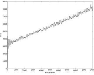
Figure 3.1: MSE using Taylorseries method Vel=2

9000

8000

7000

6000

5000

4000

3000

2000

1000

0 1000 2000 3000 4000 5000 6000 7000 8000 9000 10000 Movements

LU CO s

0

LU CO s

[image:30.612.158.480.119.386.2] [image:30.612.158.478.439.695.2]

(31)

9000

8000

7000

6000

5000

4000

3000

2000

1000

0 1000 2000 3000 4000 5000 6000 7000 8000 9000 10000 Movements

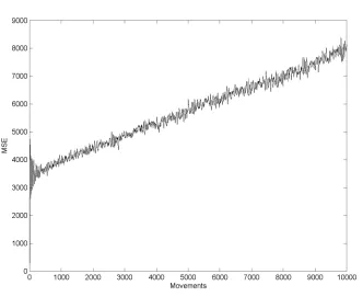
Figure 3.3: MSE using Taylorseries method Vel=10

In figures(3.43.6) we can see that the Modified Taylorseries method is improving the localization of the nodes maintaining a stable MSE during all the movements of the network. We can see that an increment of the velocity increment the MSE of the localization but is a stable increment.

LU CO s

[image:31.612.156.488.116.387.2]

(32)

8.5

7.5

6.5

5.5

0 1000 2000 3000 4000 5000 6000 7000 8000 9000 10000 Movements

Figure 3.4: MSE using Modified Taylorseries method Vel=2

64

62

60

58

56

54

52

50

48

46

44

1000 2000 3000 4000 5000 6000 7000 8000 9000 10000 Movements

8

LU CO E 7

6

LU CO E

[image:32.612.161.478.123.385.2] [image:32.612.163.475.440.692.2]

(33)

155

150

145

140

135

130

125

115

110

1051 1 1 1 1 1 1 1 1 1_I

0 1000 2000 3000 4000 5000 6000 7000 8000 9000 10000 Movements

Figure 3.6: MSE using Modified Taylorseries method Vel=10

In this simulations, the mean of neighboring nodes in each iteration of the local ization is 28.7542 nodes per NOI and the average distance of this nodes with the NOI is 6.5726m an in the next table we can see the mean of the MSE of the simulations:

Table 3.1: Mean MSE of simulations of Taylorseries method and Modified Taylorseries method without improvements

TS MTS Vel=2 5.6379 x 103_6.5788

Vel=6 5.6713 x 103_54.1282

Vel=10 5.7206 103_123.2186

[image:33.612.160.486.121.385.2]

(34)

Chapter 4 Proposed Solution

4.1. Position Estimation through Centroid

One of the first methods we will use to improve the localization of the nodes in the

network is the use of the graft method of the centroid. This method is used when the

Taylor-series or Modified Taylor-series algorithm estimate a position outside the radius

that is created with the movement of the NOI, if the velocity of the node is 2

m/s

then

this radius is equal to 2 meters. In this case, the position estimate is replaced with the

estimation made though centroid.

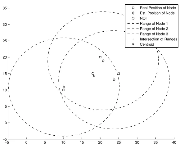
This method consist in tracing a circle with a radius equal to the measurement

range of the nodes using as the center of this circle the real position of the NOI, this is

only to determinate which neighboring nodes will participate in the localization. Then

every neighbor trace a circle with the center in the estimated position of this nodes,

then every intersection of the circles is used to build a geometric figure where the

cen-troid of this new figure is used as the new position estimation of the NOI, this process

can be seen in the figure(4.1) where the intersection of 3 estimated neighboring nodes

are used to estimate the position of the NOI.

(35)

Chapter 4. Proposed Solution.

21

−5 0 5 10 15 20 25 30 35 40

−5 0 5 10 15 20 25 30

35 Real Position of Node

Est. Position of Node NOI

[image:35.612.173.463.123.363.2]

Range of Node 1 Range of Node 2 Range of Node 3 Intersection of Ranges Centroid

Figure 4.1: Position estimation using Centroid

In the next simulations will be use the same parameters of the simulations used

in chapter 3:

Square area with an area of 10,000

m

2

Node density of 0.1

nodes/m

2

A measurement range of 10

m

A velocity that can go randomly to a maximum of 2, 6 or 10

m/s

for each node

Range measurement variance of 5

10000 Movements of all the nodes

(39)

Chapter 4. Proposed Solution.

25 Table 4.1: Mean MSE of simulations of Taylor-series method and Modified Taylor-series

method with centroid

TS

M-TS

Vel=2

1 .

5838

×

10

3

6.4743

Vel=6

1 .

6075

×

10

3

53.2546

Vel=10

1 .

6560

×

10

3

122.1188

In the table 4.2 we can see the use of the centroid in the localization of the NOI.

This data show that almost all the nodes use the centroid with the Taylor-series method,

which is the reason that the MSE is in a certain value.

Table 4.2: Use of the centroid in Taylor-series method and Modified Taylor-series

TS

M-TS

Vel=2

999.0903

94.25 Vel=6

982.13

32.13 Vel=10

956.68

17.46

4.2. Average of Estimations to Improve

Localiza-tions

The next method used to improve the localization of the NOI is to use an average

of the position estimations used in the nodes. When the NOI is estimated, is also

estimated the neighboring nodes that were used to made the estimation of the NOI,

normally when the next NOI is estimated this node uses almost all of the neighboring

nodes used in the previous estimation, and at the end of the new estimation, this nodes

updates the new position, forgetting the last update they have in previous estimations.

(40)

Chapter 4. Proposed Solution.

26 iterations of the algorithm

In the next figures the Modified Taylor-series method is used with the averaged

estimations (figures(4.8-4.10)) and then used also with the centroid (figures(4.11-4.13)).

0 1000 2000 3000 4000 5000 6000 7000 8000 9000 10000 4.5

29

0 1000 2000 3000 4000 5000 6000 7000 8000 9000 10000 70

75 80 85 90 95 100

Movements

MSE

Figure 4.13: MSE using Modified Taylor-series with averaged estimations and centroid

with a Vel=10

We can see in the table 4.3 that in this method, the centroid make little difference

improving the localization:

Table 4.3: Mean MSE of simulations of Modified Taylor-series method without centroid

and with centroid using averaged estimations

M-TS

M-TS Centroid

Vel=2

5.3009

5.2881

Vel=6

33.8392

33.7798

Vel=10

86.5084

86.4218

4.3. Use of Beacons

(44)

Chapter 4. Proposed Solution.

30 In the next simulations, the parameters will be the same, with the exception that

will include a certain percent of beacons in the network. For this simulations will use

a 5% of the nodes of the network:

Square area with an area of 10,000

m

2

Node density of 0.1

nodes/m

2

A measurement range of 10

m

A velocity that can go randomly to a maximum of 2, 6 or 10

m/s

for each node

Range measurement variance of 5

10000 Movements of all the nodes

5% of beacons

In the next figures(4.14-4.16) will use only the Taylor-series method without any

improvement and in the figures(4.17-4.19) the Modified Taylor-series is show.

0 1000 2000 3000 4000 5000 6000 7000 8000 9000 10000 0

33

0 1000 2000 3000 4000 5000 6000 7000 8000 9000 10000 105

110 115 120 125 130 135 140 145

Movements

[image:47.612.173.465.126.359.2]

MSE

Figure 4.19: MSE using Modified Taylor-series method Vel=10 and beacon density of

5%

We can see that alone, the beacons can’t make much a difference with respect to

the figures(3.1-3.6) and the table 4.4.

Table 4.4: Mean MSE of simulations of Taylor-series method and Modified Taylor-series

method with beacons

TS

M-TS

Vel=2

5 .

6553

×

10

3

6.5667

Vel=6

5 .

7688

×

10

3

53.7176

Vel=10

5 .

8297

×

10

3

121.4451

(48)

Chapter 4. Proposed Solution.

34

0 1000 2000 3000 4000 5000 6000 7000 8000 9000 10000 0

100 200 300 400 500 600 700

Movements

[image:48.612.171.466.125.361.2]

MSE

Figure 4.20: MSE using Taylor-series method with centroid, Vel=2 and beacon density

of 5%

0 1000 2000 3000 4000 5000 6000 7000 8000 9000 10000 0

36

0 1000 2000 3000 4000 5000 6000 7000 8000 9000 10000 44

46 48 50 52 54 56 58 60 62

Movements

[image:50.612.176.464.129.359.2]

MSE

Figure 4.24: MSE using Modified Taylor-series method with centroid, Vel=6 and beacon

density of 5%

0 1000 2000 3000 4000 5000 6000 7000 8000 9000 10000 105

110 115 120 125 130 135 140 145

Movements

MSE

[image:50.612.172.464.436.669.2]

(51)

Chapter 4. Proposed Solution.

37 In the figures(4.20-4.22) and table 4.5, we can see that the incursion of the beacons

in the Taylor-series method with centroid improve the localization in the network, but

in have a minimum impact in the localization with the Modified Taylor-series method

with centroid as seen in the previous figures(4.23-4.25).

Table 4.5: Mean MSE of simulations of Taylor-series method and Modified Taylor-series

method with the use of centroid and beacons

TS

M-TS

Vel=2

216.9250

6.6017

Vel=6

103.0274

53.0159

Vel=10 112.4107

120.3012

Now we will simulate the network using Modified Taylor-series with averaged

es-timations, with and without centroid. The figures(4.26-4.28) will not use the centroid

and figures(4.29-4.31) will use the centroid.

0 1000 2000 3000 4000 5000 6000 7000 8000 9000 10000 4.6

39

0 1000 2000 3000 4000 5000 6000 7000 8000 9000 10000 4.5

5 5.5 6

Movements

[image:53.612.172.466.130.359.2]

MSE

Figure 4.29: MSE using Modified Taylor-series method with averaged estimations and

centroid, Vel=2 and beacon density of 5%

0 1000 2000 3000 4000 5000 6000 7000 8000 9000 10000 29

30 31 32 33 34 35 36 37 38 39

Movements

MSE

[image:53.612.175.463.436.667.2]

(54)

Chapter 4. Proposed Solution.

40

0 1000 2000 3000 4000 5000 6000 7000 8000 9000 10000 75

80 85 90 95 100

Movements

[image:54.612.174.465.124.361.2]

MSE

Figure 4.31: MSE using Modified Taylor-series method with averaged estimations and

centroid, Vel=10 and beacon density of 5%

In the table 4.6 is showed that the centroid doesn’t improve too much in the

localization:

Table 4.6: Mean MSE of simulations of Modified Taylor-series method without centroid

and with centroid using beacons and averaged estimations

M-TS

M-TS Centroid

Vel=2

5.3013

5.3216

Vel=6

33.5193

33.4984

Vel=10

85.1387

84.9934

4.4. Comparative between Simulations

(55)

Chapter 4. Proposed Solution.

41 The first comparative is with the Taylor series method with and without the use

of beacons:

0 1000 2000 3000 4000 5000 6000 7000 8000 9000 10000 0

10 20 30 40 50 60 70 80 90 100

Movements

RMSE

TS Vel=2 TS Vel=6 TS Vel=10

Figure 4.32: RMSE using Taylor-series method

0 1000 2000 3000 4000 5000 6000 7000 8000 9000 10000 0

10 20 30 40 50 60 70 80 90 100

RMSE

Movements TS Vel=2 & Beacons 5%

TS Vel=6 & Beacons 5% TS Vel=10 & Beacons 5%

Figure 4.33: RMSE using Taylor-series method and beacon density of 5%

(56)

Chapter 4. Proposed Solution.

42 the use of beacons:

0 1000 2000 3000 4000 5000 6000 7000 8000 9000 10000 0

5 10 15 20 25 30 35 40 45

Movements

RMSE

TS Vel=2 with Centroid TS Vel=6 with Centroid TS Vel=10 with Centroid

Figure 4.34: RMSE using Taylor-series method with centroid

0 1000 2000 3000 4000 5000 6000 7000 8000 9000 10000 0

5 10 15 20 25 30

Movements

RMSE

[image:56.612.163.483.149.376.2]

TS Vel=2 with Centroid & Beacon 5% TS Vel=6 with Centroid & Beacon 5% TS Vel=10 with Centroid & Beacon 5%

Figure 4.35: RMSE using Taylor-series method with centroid and beacon density of 5%

(57)

Chapter 4. Proposed Solution.

43 individually the improvement doesn’t have a great impact in the localization of the

nodes.

Next we have the comparative using the Modified Taylor series method:

0 1000 2000 3000 4000 5000 6000 7000 8000 9000 10000 0

2 4 6 8 10 12

Movements

RMSE

M−TS Vel=2 M−TS Vel=6 M−TS Vel=10

Figure 4.36: RMSE using Modified Taylor-series method

0 1000 2000 3000 4000 5000 6000 7000 8000 9000 10000 0

2 4 6 8 10 12

density of 5%

M−TS Average Vel=2 with Centroid & Beacons 5% M−TS Average Vel=6 with Centroid & Beacons 5% M−TS Average Vel=10 with Centroid & Beacons 5%

Figure 4.43: RMSE using Averaged Estimations on Modified Taylor-series method with

centroid and beacon density of 5%

(61)

C

h

a

p

te

r

4 .

P

ro

p

o

se

d

S

o

lu

ti

o

n

.

47 sim

u

la

tio

n

s.

In

th

e

fi

gu

re

4.

44 ar

e

ex

p

re

ss

ed

th

is

re

su

lt

s

to

ma

ke

a

ea

sy

co

mp

ar

at

iv

e

b

et

w

ee

n

al

l

th

e

me

th

o

d

s

u

se

d

in

th

is

w

or

k

.

Al

so

in

fi

gu

re

4.

45 ar

e

sh

ow

ed

th

e

st

an

d

ar

d

ev

ia

tio

n

of

th

e

R

M

S

E

of

th

e

sim

u

la

tio

n

s,

th

is

re

su

lt

s

ar

e

ob

ta

in

ed

fr

om

th

e

re

su

lt

s

or

th

e

R

M

S

E

w

it

h

ou

t

th

e

u

se

of

th

e

M

ov

in

g

av

er

ag

e

fi

lt

er

u

se

d

in

th

e

co

mp

ar

at

iv

e

fi

gu

re

s

(4

.3

2-4.

43 ).

0 10 20 30 40 50 60 70 80 90

TS Vel= 2 TS Vel= 6 TS Vel= 10 TS Vel= 2 & Beacons 5% TS Vel= 6 & Beacons 5% TS Vel= 10 & Beacons 5% TS Vel= 2 with Centroid TS Vel= 6 with Centroid TS Vel= 10 with Centroid TS Vel= 2 with Centroid & Beacons 5% TS Vel= 6 with Centroid & Beacons 5% TS Vel= 10 with Centroid & Beacons 5% M-TS Vel= 2 M-TS Vel= 6 M-TS Vel= 10 M-TS Vel= 2 & Beacons 5% M-TS Vel= 6 & Beacons 5% M-TS Vel= 10 & Beacons 5% M-TS Vel= 2 with Centroid M-TS Vel= 6 with Centroid M-TS Vel= 10 with Centroid M-TS Vel= 2 with Centroid & Beacons 5% M-TS Vel= 6 with Centroid & Beacons 5% M-TS Vel= 10 with Centroid & Beacons 5% M-TS Avg. Est. Vel= 2 M-TS Avg. Est. Vel= 6 M-TS Avg. Est. Vel= 10 M-TS Avg. Est. Vel= 2 & Beacons 5% M-TS Avg. Est. Vel= 6 & Beacons 5% M-TS Avg. Est. Vel= 10 & Beacons 5% M-TS Avg. Est. Vel= 2 with Centroid M-TS Avg. Est. Vel= 6 with Centroid M-TS Avg. Est. Vel= 10 with Centroid M-TS Avg. Est. Vel= 2 with Centroid & Beacons 5% M-TS Avg. Est. Vel= 6 with Centroid & Beacons 5% M-TS Avg. Est. Vel= 10 with Centroid & Beacons 5%

[image:61.792.230.488.121.518.2]

(62)

C

h

a

p

te

r

4 .

P

ro

p

o

se

d

S

o

lu

ti

o

n

.

48

0 2 4 6 8 10 12

TS Vel= 2 TS Vel= 6 TS Vel= 10 TS Vel= 2 & Beacons 5% TS Vel= 6 & Beacons 5% TS Vel= 10 & Beacons 5% TS Vel= 2 with Centroid TS Vel= 6 with Centroid TS Vel= 10 with Centroid TS Vel= 2 with Centroid & Beacons 5% TS Vel= 6 with Centroid & Beacons 5% TS Vel= 10 with Centroid & Beacons 5% M-TS Vel= 2 M-TS Vel= 6 M-TS Vel= 10 M-TS Vel= 2 & Beacons 5% M-TS Vel= 6 & Beacons 5% M-TS Vel= 10 & Beacons 5% M-TS Vel= 2 with Centroid M-TS Vel= 6 with Centroid M-TS Vel= 10 with Centroid M-TS Vel= 2 with Centroid & Beacons 5% M-TS Vel= 6 with Centroid & Beacons 5% M-TS Vel= 10 with Centroid & Beacons 5% M-TS Avg. Est. Vel= 2 M-TS Avg. Est. Vel= 6 M-TS Avg. Est. Vel= 10 M-TS Avg. Est. Vel= 2 & Beacons 5% M-TS Avg. Est. Vel= 6 & Beacons 5% M-TS Avg. Est. Vel= 10 & Beacons 5% M-TS Avg. Est. Vel= 2 with Centroid M-TS Avg. Est. Vel= 6 with Centroid M-TS Avg. Est. Vel= 10 with Centroid M-TS Avg. Est. Vel= 2 with Centroid & Beacons 5% M-TS Avg. Est. Vel= 6 with Centroid & Beacons 5% M-TS Avg. Est. Vel= 10 with Centroid & Beacons 5%

Typ

e

o

f Sim

Std. Deviation of RMSE

(63)

Chapter 5 Conclusions

5.1. Conclusions

We can see trough all the simulations and results of the tests in the networks, Modified Taylor series method give us the best performance in te localization of the nodes in a network, as we can see in the tables 5.1 and 5.2 where the best performance obtained trough the simulations is when we use the Modified Taylor series method with the use of the averaged estimations and the beacons and centroid contribute little in the improvement of the MSE.

Table 5.1: Mean MSE of simulations without beacons

TS MTS TS cent MTS cent MTS avg MTS avg cent Vel=2 5.6379 x 103

6.5788 1.5838 x 103

6.4743 5.3009 5.2881 Vel=6 5.6713 x 103_{54.1282 1.6075 x 10}3_{53.2546 33.8392 33.7798}

Vel=10 5.7206 x 103_{123.2186 1.6560 x 10}3_{122.1188 86.5084 86.4218}

(64)

Chapter 5. Conclusions. 50

Table 5.2: Mean MSE of simulations with beacons

TS MTS TS cent MTS cent MTS avg MTS avg cent Vel=2 5.6553 x 103

6.5667 216.9250 6.6017 5.3013 5.3216 Vel=6 5.7688 x 103_{53.7176 103.0274 53.0159 33.5193 33.4984}

Vel=10 5.8297 x 103_{121.4451 112.4107 120.3012 85.1387 84.9934}

With this, one conclusion that we can find is that the use of centroid and bea¬ cons doesn't improve substantially the MSE in the network, with this, the use of this methods only increase the use of power and time to process the information, wasting resources where the use of the Modified Taylor series method with averaged estimations could be a more efficient way of improve the localization in the network.

5.2. Future Research

(65)

Bibliography

[1] Y Sankarasubramaniam I. Akyildiz, W . Su and E. Cayirci. Wireless sensor net works: A survey. Computer Networks J., 38(4):393422, Mar 2002.

[2] N.S. Correal and N. Patwari. Wireless sensor networks: Challenges and opportu nities. Virginia Tech Symp. Wireless Personal Communications, pages 19, June 2001.

[3] N.S. Correal M. Perkins and R.J. O'Dea. Emergent wireless sensor network limi tations: A plea for advancement in core technologies. IEEE Sensors, 2:15051509, June 2002.

[4] C. K. Toh. Ad Hoc Mobile Wireless Networks. Prentice Hall, 2002.

[5] Ramsesh Govindan Deborah Estrin and John Heidemann. Scalable coordination in sensor networks. Technical report, USC/ISI, 1999.

[6] John Heidemann Ya Xu and Deborah Estrin. Adaptive energyconserving routing for multihop ad hoc networks. Technical report, USC/ISI, 2000.

[7] W . Guo G. Sun, J. Chen and K.J.R. Liu. Signal processing techniques in network aided positioning. IEEE Signal Processing Mag., 22(4):1223, July 2005.

[8] D. Niculescu and B. Nath. Ad hoc positioning system (aps) using aoa. Proc. IEEE INFOCOM 2003, 3:17341743, 2003.

[9] D. Estrin N. Bulusu, J. Heidemann and T. Tran. Selfconfigurating localization systems: Design and experimental evaluation. ACM Trans. Embedded Comput. Syst., 3(1):2460, Feb 2004.

[10] A. Sabharwal A. Chakrabarti and B. Aazhang. Using predictable observer mobility for power efficient design of sensor networks. Proc. IPSN 2003, pages 129145.

(66)

Bibliography. 52 [11] M.L. Sichitiu and V. Ramadurai. Localization of wireless sensor networks with a

mobile beacon. Technical report, Center of Advances in Computing and Commu¬ nications (CACC), 2003.

[12] S. Pattem A. Galstyan, B. Krishnamachari and K. Lerman. Distributed online localization in sensor networks using a moving target. Proc. Information Processing in Sensor Networks (IPSN2004)., pages 6170, 2004.

[13] Spyros Kyperountas Alfred O. Hero III Randolph L. Moses Neal Patwari, Joshua N. Ash and Neiyer S. Correal. Locating the nodes. IEEE Signal Processing Mag.,

22(4):5469, July 2005.

[14] Piscataway. Coherence and Time Delay Estimation. IEEE Press, 1993.

[15] W . H. Foy. Positionlocation solution by taylorseries estimations. IEEE Transac¬ tions on Aerospace and Electronic Systems, AES12:187194, March 1976.

[16] Don J. Torrieri. Statistical theory of passive location systems. IEEE Transactions on Aerospace and Electronic Systems, AES20(2):183197, March 1984.

[17] L. Kovavisaruch and K. C. Ho. Modified taylorseries method for source and receiver localization using tdoa measurements with erroneous receiver positions.

Beacon Free Localization in mobile Ad-Hoc Networks Based on a Modified Taylor Series Multilateration Technique-Edición Única

Beacon Free Localization in mobile Ad­Hoc Networks Based on

a Modified Taylor Series Multilateration Technique­Edición

Única

Title

Beacon Free Localization in mobile Ad­Hoc Networks

Based on a Modified Taylor Series Multilateration

Technique­Edición Única

Authors

José Manuel Rodríguez Delgado

Affiliation

Tecnológico de Monterrey, Campus Monterrey

Issue Date

2008­11­01

Item type

Tesis

Rights

Open Access

Downloaded

19­Jan­2017 01:52:35

Beacon free localization in mobile Ad­Hoc networks

based on a modified Taylor series multilateration

technique

Master of Science in Electronic Engineering

Jose Manuel Rodriguez Delgado

Thesis

Major in Telecommunications

TECNOLÓGICO

DE MONTERREY.

Thesis Committee:

Acknowledgments

JOSÉ MANUEL RODRÍGUEZ DELGADO

Beacon free localization in mobile Ad­Hoc networks

based on a modified Taylor series multilateration

technique

Contents

List of Figures

3.1. MSE using Taylor-series method Vel=2 . . . .

16

3.2. MSE using Taylor-series method Vel=6 . . . .

16

3.3. MSE using Taylor-series method Vel=10 . . . .

17

3.4. MSE using Modified Taylor-series method Vel=2 . . . .

18

3.5. MSE using Modified Taylor-series method Vel=6 . . . .

18

3.6. MSE using Modified Taylor-series method Vel=10 . . . .

19

4.1. Position estimation using Centroid . . . .

21

4.2. MSE using Taylor-series method and Centroid with a Vel=2 . . . .

22

4.3. MSE using Taylor-series method and Centroid with a Vel=6 . . . .

22

4.4. MSE using Taylor-series method and Centroid with a Vel=10 . . . .

23

4.5. MSE using Modified Taylor-series method and Centroid with a Vel=2 .

23

4.6. MSE using Modified Taylor-series method and Centroid with a Vel=6 .

24

4.7. MSE using Modified Taylor-series method and Centroid with a Vel=10

24

4.8. MSE using Modified Taylor-series with averaged estimations with a Vel=2 26

4.9. MSE using Modified Taylor-series with averaged estimations with a Vel=6 27

4.10. MSE using Modified Taylor-series with averaged estimations with a Vel=10 27

4.11. MSE using Modified Taylor-series with averaged estimations and

cen-troid with a Vel=2 . . . .

28

4.12. MSE using Modified Taylor-series with averaged estimations and

cen-troid with a Vel=6 . . . .

28

4.13. MSE using Modified Taylor-series with averaged estimations and

cen-troid with a Vel=10 . . . .

29

4.14. MSE using Taylor-series method Vel=2 and beacon density of 5% . . .

30

4.15. MSE using Taylor-series method Vel=6 and beacon density of 5% . . .

31

4.16. MSE using Taylor-series method Vel=10 and beacon density of 5% . . .

Beacon Free Localization in mobile AdHoc Networks Based on

a Modified Taylor Series Multilateration TechniqueEdición

Beacon Free Localization in mobile AdHoc Networks

TechniqueEdición Única

20081101

19Jan2017 01:52:35

Beacon free localization in mobile AdHoc networks

Beacon free localization in mobile AdHoc networks