Checking unimodality using isotonic regression: an
application to breast cancer mortality rates
Rueda1, C., Ugarte2∗,3, M.D. and Militino2,3, A.F. 1Department of Statistics and Operations Research, Valladolid University
Facultad de Ciencias, 47005 Valladolid, Spain
2Department of Statistics and Operations Research, Public University of Navarre 3INAMAT, Public University of Navarre
Campus de Arrosadia, 31006 Pamplona, Spain e-mail2∗: [email protected]
Abstract
In some diseases it is well-known that a unimodal mortality pattern exists. A clear ex-ample in developed countries is breast cancer, where mortality increased sharply until the nineties and then decreased. This clear unimodal pattern is not necessarily applicable to all regions within a country. In this paper, we develop statistical tools to check if the unimodal-ity pattern persists within regions using order restricted inference. Break points as well as confidence intervals are also provided. In addition, a new test for checking monotonicity against unimodality is derived allowing to discriminate between a simple increasing pattern and an up-then-down response pattern. A comparison with the widely used joinpoint regres-sion technique under unimodality is provided. We show that the joinpoint technique could fail when the underlying function is not piecewise linear. Results will be illustrated using age-specific breast cancer mortality data from Spain in the period 1975-2005.
Keywords: change point, isotonic regression, order restricted inference, temporal trends, joint point regression, segmented regression
1
Introduction
The analysis of mortality and incidence trends is very informative when analyzing cancer inci-dence or mortality (Ruiz-Medina et al., 2014). Changes in the (temporal) trend could be due to many reasons like an improvement in the treatment of the disease, better habits or life style in the population or just the effect of a screening program. The detection of these changes in trends is then of great interest for epidemiologists and public health researchers. In the epi-demiological literature, the classical procedure used to detect trend changes is called joinpoint regression. The joinpoint regression software developed by the National Cancer Institute of the United States is widely used (Molodecky et al., 2012, Simard et al., 2012, de Souza et al., 2013, Hur et al., 2013, L´opez-Campos et al., 2013). The implemented method is developed by Kim et al. (2000), although the basics of the method are older (Sprent, 1961, Hudson, 1966, Feder, 1975, Lerman, 1980). The objective of the joinpoint technique is to find not only trend changes
Manuscript
but also its location. In many applications of regression in different fields, the response and the explanatory variable exhibit a unimodal pattern, i.e., the response variable increases up to a certain unknown point and then decreases. This up-then-down response pattern is usually called an umbrella or unimodal ordering. Unimodal regression often arises in the analysis of epidemiological data, such as dose response studies, where the response increases with the dose until a certain level and then decreases. Additional examples are given by Morton-Jones et al.(2000), Banerjee et al. (2009) or Gunn and Dunson (2005). Many of these applications are aimed to locate the peak and to test the null hypothesis of a simpler increasing pattern. An interesting case is the analysis of surveillance data from an epidemic (Bock et al., 2008), where the interest relies on an early detection of the peak of the epidemic that can be accomplished with thep-value of the mentioned test. Different parametric approaches can be used to estimate a unimodal relationship and the corresponding peak, such as fitting a quadratic or a joinpoint regression. Nonparametric approaches can also be used. For example, Ugarte et al (2010) choose the peak as a simple choice of selecting the maximum of a smoothed version of the data and more recently K¨ollmann et al. (2012) use splines for the same goal. Both, the parametric and the nonparametric solutions have important drawbacks. The parametric approaches require a careful choice of the form of the function giving biased estimates of the location of the peak under an erroneous specification of the function. The nonparametric approaches are not easy to implement and require user-specified choices, such as bandwidth, smoothing parameters or the number and placement of knots. The adopted proposal of this paper is a semiparametric regression approach with specific advantages. It is very simple and it gives a location estimate of the peak without assuming a specific form of the regression function.
The goal of this paper is threefold. First, to propose the isotonic regression (Robertson et al.,1988) as a sensible tool that outperforms joinpoint regression in unimodal patterns. Sec-ond, to derive conditional tests for checking unimodality and for testing monotonicity against unimodality. Akaike Information criterion (AIC) measures are also provided and confidence in-tervals for the peaks are given using a parametric bootstrap approach. Third, to analyze trend changes and its location in breast cancer mortality.
Several authors have dealt with related problems using the isotonic regression for monotone regression models or for alternative shape constraints. Some representative references are Brunk (1970), Dykstra (1983), Hastie and Tibshirani (1986), Bachetti (1989), Huang (2002), Andersson et al. (2004), Meyer (2008), Shively et al. (2011) and Rueda and Lombard´ıa (2012) among many others. There has been also considerable previous work on procedures testing homogeneity against monotonicity or unimodality (see for example Basso and Salmaso, 2011, Shi, 1988 and Wolfe, 2006), but the problem of considering testing monotonicity against unimodality has not been studied yet. This particular test will be very useful in the application considered in this paper. Although it is known that breast cancer mortality rates show a clear unimodality pattern in some developed countries (Malvezzi et al. 2012), we are particularly interested here in testing if this unimodality pattern persists in small areas within the country. The methodology derived will be also useful to analyze data from a variety of applications in many fields whenever the interest relies on checking if the functional relationship between the response and the explanatory variable exhibit a unimodal or monotone pattern.
condi-tional tests for checking unimodality and testing monotonicity against unimodality are derived. Section 4 illustrates the methodology analyzing breast cancer mortality data in Spain and its Autonomous Regions in the period 1975-2005. A comparison with the results obtained using joinpoint regression is also provided. A discussion closes this paper.
2
Isotonic regression for fitting and testing temporal trends in
mortality rates
Let Yt be the number of deaths in year t, fromt=t1, . . . , tn in a given region. It is commonly
assumed that Yt is Poisson distributed with mean µt = ntrt, where rt is the unknown rate of
mortality and nt is the population at risk. Once the rate is estimated at each year we could
represent the mortality temporal trend in that particular region. Our interest here relies on checking if there exists a break-point in the temporal trend, and if it does, to estimate it. In what follows a brief introduction of the underlying methodology is provided. Letr= (rt1, . . . , rtn) be
the vector of rates. LetM ={r∈ <n|rt1 ≤ · · · ≤rt
n} be the set representing the monotonicity
of rates over the study period (this means that there is not a rate trend change over the years) and U = {r ∈ <n|r
t1 ≤ · · · ≤ rq ≥ rq+1 ≥ · · · ≥ rtn, t1 ≤ q ≤ tn} be the set representing
a temporal pattern of unimodality. To check for the presence of a unimodality pattern and therefore, the existence of a break point in the rate temporal trend r, we consider first the simple case where an initial guess for the mode or break point (ψ), ψ0 =q is given. Consider
the following hypotheses
H0q:rt1 ≤ · · · ≤rq=rq+1=· · ·=rtn,
H1q:rt1 ≤ · · · ≤rq≥rq+1≥ · · · ≥rtn,
H2 :r∈ <n.
Two tests will be performed. The first test checks for the existence of unimodality. Namely
H1q vs. H2−H1q (1)
and the second one checks for the presence of a break-point before the end of the period under study
H0q vs. H1q−H0q. (2)
The maximum likelihood estimatorsbr0q andbr1q under H0q and H1q are obtained by solving
max
{r∈<n|r
t1≤···≤rq=rq+1=···=rtn}
l(r) (3)
and
max
{r∈<n|r
t1≤···≤rq≥rq+1≥···≥rtn}
wherel(r) is the Poisson log-likelihood given by
l(r) =
tn X
t=t1
ytlog (rt) +ytlog (nt)−log (yt!)−rtnt
!
.
In the case of ψ being unknown, a plug-in approach is performed. Firstly, the observed mode
b
ψ=q is derived by solving
max
t1≤q≤tn
max
{r∈<n|r
t1≤···≤rq≥rq+1≥···rtn} l(r)
(5)
and then, it is plugged in tests (1) and (2). In the case that (5) has multiple solutions, the highest value is selected as the mode. The solution to the optimization problems (3), (4) and (5) is achieved using isotonic regression. These problems can be solved as a weighted least squares fit of the observed ratesv= (vt1, . . . , vtn), wherevt=yt/nt and the weights are given bywt=nt,
subject to monotonicity or unimodality constraints. A convenient algorithm for carrying this out is stated by Shi (1988) and it has been implemented in the R package Iso (see Turner, 2013). Confidence intervals (CI) can be also computed. The methodology to derive CIs under restrictions has not been treated very extensively in the literature. Some interesting papers are written by Hwang and Peddada (1994), Peddada (1997) and Pan (1997). More recently, Strand et al. (2010) compare alternative proposals to derive CI for monotone regression pointing out the parametric bootstrap as the best choice. Parametric bootstrap has been considered in this paper to obtain CIs.
2.1 The AIC criterion and the degrees of freedom
To choose between a monotoneM or a unimodalU pattern, an AIC-type criterion similar to the AIC criterion (Akaike, 1973) used in linear regression is proposed. This alternative is simpler than the test approach we will derive in the next section. A general definition of this criterion for a restricted statistical model with parameter spacer∈K, whereKis any subset in<nis given by AIC(brK) =−2l(
br
K) + 2g(D
K(v)),l(.) is the log-likelihood of the estimated model,g(DK(v)) is
a penalty term, gis a real function often defined as g(x) =x and DK(v) are the model degrees
of freedom, also called the divergence. They are generally defined as DK(v) = tn P
t=t1 ∂br
K(v) ∂vt ,
and particularly here DK(v) = n−][t,br
K t = br
K
t+1]. The use of the AIC statistic in isotonic
models backs to Anraku (1999), yet posterior modifications have been introduced (see Zhao and Peng, 2002, and Liu et al. 2009). In this paper, the idea of Kato (2009) and Rueda (2013) proposing a penalty term equal to 2DK(v) in a regression context has been applied. Although
computing DK(v) is straightforward in most parametric models, the restricted case is not so
3
The conditional likelihood ratio test
In this section the conditional tests for testing (1) and (2) are derived. Initially, normal dis-tributions with known variances are assumed. The case of unknown variances and the Poisson model as well as other exponential distributions will be considered as extensions of this simple model. Let us assume thatYt∼N(rt, σt), whereσtare known parameters. Here, the maximum
likelihood estimate (MLEs) ofr underH0q and H1q are the solutions to the optimization
prob-lems (3) and (4) respectively, where now l(r) is the normal log-likelihood. The MLEs are also obtained through the isotonic regression of v= (v1, . . . , vtn), where vt=yt and wt= 1/σt.
Let us consider H0 : r ∈ K0 and Ha : r ∈ Ka, where K0 and Ka are any subsets in <n, and
the testing problem H0 vs. Ha−H0. For this general testing problem the likelihood ratio
statisticT is defined as
T = 2(l(ˆra)−l(ˆr0)),
where l(.) is the normal log-likelihood and ˆra and ˆr0 are the MLE under the alternative and the null hypothesis respectively. Let D = DKa(v) −DK0(v) be the data-dependent degrees
of freedom of T. Under suitable regularity conditions, the distribution of T has proven to be conditionally distributed as a χ2d when rt1 = · · · =rtn (in what follows we denote r0 a vector
whose components are equal), and dis the observed value ofD, i.e,
prr0(T ≤c|D=d) =pr(χ
2
d≤c),
(see Men´endez et al., 1992 and Hu and Wright, 1994). The conditionalα level test rejects when
T ≥c(d) wherec(d) is defined as the 1−α0 percentile of theχ2ddistribution such that
α0 =pr χ2d≥c(d)= α
1−prr0(T = 0)
. (6)
The parameter configuration r0 has proven to be the least favorable configuration (LFC) of
parameters under the null hypothesis for the likelihood ratio test (LRT) in regular testing problems. Besides, it has been shown that, asymptotically, the LFC is alsor0 for the conditional
test under non oblique hypothesis (see Wollan and Dykstra, 1986 and Men´endez et al., 1991). This important fact guarantees that the conditional test is asymptotically anαlevel test allowing to obtain a p-value from a χ2d distribution. When prr0(T = 0) is a very small number for
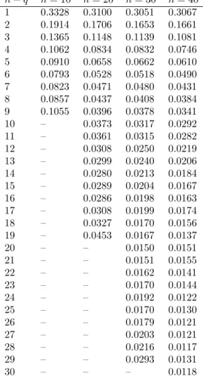
Table 1: pr(TMq = 0) for different values of n and q, equal weights and independent N(0,1)
distributions
n−q n= 10 n= 20 n= 30 n= 40
1 0.3328 0.3100 0.3051 0.3067 2 0.1914 0.1706 0.1653 0.1661 3 0.1365 0.1148 0.1139 0.1081 4 0.1062 0.0834 0.0832 0.0746 5 0.0910 0.0658 0.0662 0.0610 6 0.0793 0.0528 0.0518 0.0490 7 0.0823 0.0471 0.0480 0.0431 8 0.0857 0.0437 0.0408 0.0384 9 0.1055 0.0396 0.0378 0.0341
10 – 0.0373 0.0317 0.0292
11 – 0.0361 0.0315 0.0282
12 – 0.0308 0.0250 0.0219
13 – 0.0299 0.0240 0.0206
14 – 0.0280 0.0213 0.0184
15 – 0.0289 0.0204 0.0167
16 – 0.0286 0.0198 0.0163
17 – 0.0308 0.0199 0.0174
18 – 0.0327 0.0170 0.0156
19 – 0.0453 0.0167 0.0137
20 – – 0.0150 0.0151
21 – – 0.0151 0.0155
22 – – 0.0162 0.0141
23 – – 0.0170 0.0144
24 – – 0.0192 0.0122
25 – – 0.0170 0.0130
26 – – 0.0179 0.0121
27 – – 0.0203 0.0121
28 – – 0.0216 0.0117
29 – – 0.0293 0.0131
3.1 Testing unimodality against <n
In this section testing problem (1) is considered. Let T1q be the LR statistic, the conditional
test rejects H1q when T1q ≥c(d) and c(d) is defined in (6). Problem (1) is regular because the
alternative is a linear subspace. Therefore, following similar arguments to those given by Iverson and Harp (1987) it can be proved that the level of the test is attained atr0 and that the size of
the test for other parameter values in the null hypothesis is asymptotically smaller thanα.
Remark 1 A small practical difficulty with the conditional test just defined is the evaluation of
prr0(T1q = 0), which depends on wt, q, and n. It can be computed by simulation. Moreover,
taking into account thatpr(v∈ {rt1 ≤ · · · ≤rq ≥rq+1≥ · · · ≥rtn})≤pr(v∈T O), whereT O is
the tree order cone (see Robertson et al., 1988), it is easy to prove that prr0(T1q= 0)→n→∞ 0.
In particular, ifwt=w,prr0(T1q= 0)≤
1
(n−1)!. Therefore, to simplify computation, in scenarios with moderate or large n, c(d) is simply defined as the 1−α percentile of the χ2d distribution. The loss of power is not significant for moderate or large n values.
Remark 2 i) There is a natural extension when working with normal distributions with un-known but common variances. The conditional test is easy to formulate using the results by Men´endez et al. (1992). The F distribution is then used instead of the chi-squared distribution for the test statistic.
ii) For the case of the Poisson distribution and other exponential families, the results above are true when (nt) is big enough. The fact that the asymptotic distribution of the LR statistic is the
same as the one in the normal case (see Robertson et al., 1988; Chapter 4) guarantees that the results are asymptotically valid in exponential families.
3.2 Testing monotonicity against unimodality
In this section testing problem (2) is considered. The corresponding LR statistic is denoted by
T0q. This is a non regular problem as both hypotheses are defined by cones that are not linear
subspaces. However, we will show that also in this case the conditional test can be successfully applied. The conditional test rejects H0q when T0q ≥c(d), where c(d) is defined as the 1−α0
percentile of a χ2d distribution with α0 = 1−pr α
r0(T0q=0). Denote by Πq(r) the size in r of the
conditional test defined for testing problem (2). Then,
Πq(r) =
X
d
prr(T0q ≥c(d)|D=d)prr(D=d). (7)
Theorem 3 proves two results. Firstly, we show that the distribution of the LR statistic T0q
conditioned toD=dis aχ2dand subsequently, that the size of the conditional test forr0 equals
α. Moreover, it is also possible to prove that the size of the conditional test is smaller thanαfor other parameter values in the null hypothesis, using both simulation and asymptotic theoretical results (Men´endez et al., 1991).
Theorem 3 Let T0q be the LR statistic for testing H0q against H1q−H0q and Πq the function
defined in (7). Then, we have: i) prr0(T0q≥c|D=d) =pr χ
2
d≥c
Remark 4 To use the test in practice, prr0(T0q = 0)needs to be computed. For givenn,q, and
wi it can be easily obtained by simulation (see Tables 1 and 2).
Remark 5 There is a natural extension of these results when working with normal distribu-tions with unknown but common variances. Moreover, results are also asymptotically valid in exponential families (Robertson et al., 1988, Chapter 4).
Table 2: prW(TMq = 0) for n= 31 and different values of q and wt,1 ≤ t ≤31. Independent N(0, sdt), sdt= 1/√wt distributions
n−q wt= 1 wt=t wt=n−t+ 1 wt=nt
1 0.3204 0.3260 0.3277 0.3131
2 0.1657 0.1738 0.1427 0.1597
3 0.1113 0.1194 0.0802 0.1089
4 0.0832 0.0894 0.0507 0.0796
5 0.0678 0.0746 0.0343 0.0656
6 0.0556 0.0628 0.0262 0.0545
7 0.0471 0.0544 0.0197 0.0464
8 0.0390 0.0463 0.0157 0.0391
9 0.0368 0.0432 0.0136 0.0370
10 0.0347 0.0387 0.0119 0.0341
11 0.0295 0.0352 0.0073 0.0299
12 0.0259 0.0329 0.0076 0.0263
13 0.0249 0.0299 0.0084 0.0247
14 0.0236 0.0292 0.0070 0.0238
15 0.0214 0.0262 0.0055 0.0224
16 0.0208 0.0256 0.0051 0.0208
17 0.0183 0.0237 0.0052 0.0188
18 0.0187 0.0232 0.0055 0.0189
19 0.0185 0.0237 0.0052 0.0191
20 0.0177 0.0206 0.0044 0.0181
21 0.0156 0.0198 0.0046 0.0163
22 0.0160 0.0177 0.0052 0.0162
23 0.0165 0.0175 0.0058 0.0171
24 0.0157 0.0157 0.0060 0.0161
25 0.0157 0.0153 0.0053 0.0153
26 0.0159 0.0142 0.0055 0.0161
27 0.0180 0.0127 0.0069 0.0178
28 0.0196 0.0112 0.0076 0.0198
29 0.0239 0.0121 0.0105 0.0239
4
Illustration
The test derived in Section 3 is illustrated using female breast cancer mortality data from Spain in the period 1975-2005. It is known (see Malvezzi et al., 2012) that in many developed countries like Spain, breast cancer mortality increased sharply until the nineties and then decreased. In this section we are interested in testing if this unimodality pattern persists in all the Autonomous Regions of Spain. An Autonomous Region is constituted by one single or a group of provinces and it has its own local government. The problem of checking unimodality in Autonomous Regions is of interest as they have their own health system and habits and therefore some differences may be found. Isotonic regression will be also used to find break points and confidence intervals for the regions where unimodality persists. However, the common procedure to estimate break points in epidemiology is the well-known joinpoint regression model (see for example, Statistical Research and Applications Branch, National Cancer Institute, 2009), therefore, a comparison between isotonic regression and joinpoint regression will be made first, to show the reasons why isotonic regression will be used in this context. The comparison will be made analyzing both real data and simulated data under the scenario of unimodality pattern (a single break point) mimicking the real mortality data from Spain. A similar procedure is used by Turner and Wollan (1997). These authors demonstrate that the isotonic estimator of the mode is consistent, simple to understand, and performs satisfactorily in practice. In the following we show that the isotonic estimator is working well in the epidemiological context considered here. However, the joinpoint regression method has two serious drawbacks; it could be seriously biased and it is not robust because when we slightly modify the studied period, the estimator provides a different mode, in contrast to the isotonic estimator.
4.1 Comparing isotonic regression and joinpoint regression
When studying trends in mortality or incidence data, it is often of interest to uncover break points. The well-known joinpoint regression models, also called segmented regression models, have been used for this aim. These models explain the relationship between the response and the explanatory variables by means of different lines called segments. In this particular application we know in advance the existence of a single break point. In this regard, Ugarte et al. (2010) report a sharp increase of female breast cancer mortality and then a downturn around the nineties in different age-groups (< 45, 45-64, ≥ 65). The epidemiological literature also reported that the decline of breast cancer mortality in Spain is delayed when the age of the group is increased. The decline starts earlier in younger women probably reflecting the increasing survival of cases (Berrino et al., 2007). Joinpoint regression finds the break point using the following model in each age-group
yt ∼ P oisson(rtnt/100000)
log(yt) = log(nt/100000) +β0+β1t+β2(t−ψ)+ (8)
whereyt is the female mortality counts from breast cancer in a specific age-group at time t,nt
is the population at risk and rt is the corresponding mortality rate (per 100,000 individuals).
line adjusted up tothe break-point ψ and β2 is the difference-in-slopes. The nonlinear term in
(8) has an approximate intrinsic linear representation permitting to express the model as a kind of generalized linear model (Muggeo, 2003). Given an initial guess for the break point, ˜ψ, model (8) can be estimated by fitting iteratively the generalized linear model with linear predictor
log(nt/100000) +β0+β1t+β2(t−ψ˜)++γI(t >ψ˜)− (9)
whereI(·)− = −I(·) andγ is the parameter that can be understood as a re-parametrization of
ψaccounting for the break point estimation. The R packagesegmentedby Muggeo (2008) offers facilities to estimate and summarize generalized linear models with segmented relationships. It uses a method that allows to estimate simultaneously all the model parameters yielding also, at the possible convergence, the approximate full covariance matrix. In our application we have fitted the model using this package.
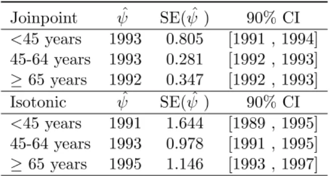
Table 3: Break point estimates of breast cancer mortality rates ˆψ as well as confidence intervals by age groups using both joinpoint and isotonic regression
Joinpoint ψˆ SE( ˆψ ) 90% CI
<45 years 1993 0.805 [1991 , 1994] 45-64 years 1993 0.281 [1992 , 1993]
≥65 years 1992 0.347 [1992 , 1993] Isotonic ψˆ SE( ˆψ ) 90% CI
<45 years 1991 1.644 [1989 , 1995] 45-64 years 1993 0.978 [1991 , 1995]
≥65 years 1995 1.146 [1993 , 1997]
Table 3 shows estimated break points, standard errors, and confidence intervals (1−α = 0.9) of the break points computed using joinpoint and isotonic regression. Surprisingly, in the join-point regression the same break join-point is found for the first two age-groups whereas for the third age group the break point is estimated one year in advance, something unexpected by epidemiologists. However, isotonic regression provides more reasonable and comprehensive re-sults. As reported in the epidemiological literature, the mortality decline starts earlier in the first (younger) age-group and from there on it suffers a delay. Computational code to fit both models are available from the authors under request.
4.1.1 Simulation study
offset, and a smooth function of the time approximated using P-splines with B-spline bases. The estimated smooth rates were considered the “true rates”. The real value of the break point is con-sidered to be the mode of the smoothed curve, more specifically the nearest integer was selected (see the first row of 1). Finally, the simulation was run following the next steps. 1) Generate 1000 samples of size nin each age-group from a Poisson distribution with mean rt=nt/100000∗rˆt,
wherent is the population at risk in yeart, and ˆrt are the estimated smooth rates. 2) Fit both
a joinpoint regression and a isotonic regression to each simulated data set and obtain break points. 3) Compute the mean bias (MB) and the root mean squared error (RMSE) of the break
point estimators. M B= 10001 P1000
j=1
ˆ
ψj−ψ
, RM SE =
r
1 1000
P1000
j=1
ˆ
ψj−ψ
2
where ˆψj
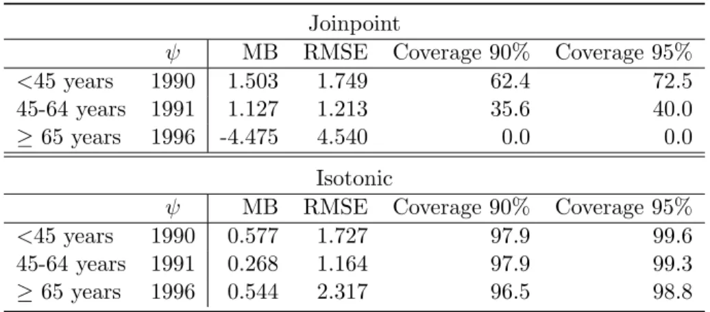
is the break point estimate using the jth simulated sample for each age-group andψ is the true value of the break point for that age-group. Results of the simulation study are given in Table 4. Graphical representation of the results are shown in the second (joinpoint regression) and third row (isotonic regression) of 1. Both, Table 4 and the graphical results point out a much larger bias for the joinpoint regression analysis. In this particular simulation study we find larger RMSE in two age groups for the joinpoint analysis. It is striking that coverage probabilities even reach the zero value for particular unimodal patterns (like the simulated pattern of the third age-group). Consequently, jointpoint regression should not be used when the underlying shape of the curve is not piecewise linear. The reason for the over-coverage in the isotonic case is due to the discrete nature of the mode distribution.
We have also analyzed breast cancer mortality rates (real data) for two more periods: 1975-2010 and 1980-2010. When representing crude rates a unimodal pattern is observed too. However, while the isotonic regression model provides the same break points in all the periods, the join-point regression model gives different break join-point estimates depending on the period. In this sense, we may affirm that the isotonic regression model is robust.
Table 4: MB, RMSE, and coverage probabilities using joinpoint and isotonic regression. The first column gives the true break point ψin each age-group
Joinpoint
ψ MB RMSE Coverage 90% Coverage 95%
<45 years 1990 1.503 1.749 62.4 72.5 45-64 years 1991 1.127 1.213 35.6 40.0
≥65 years 1996 -4.475 4.540 0.0 0.0
Isotonic
ψ MB RMSE Coverage 90% Coverage 95%
<45 years 1990 0.577 1.727 97.9 99.6 45-64 years 1991 0.268 1.164 97.9 99.3
3.0
3.5
4.0
4.5
Spain (<45 years)
1975 1980 1985 1990 1995 2000 2005
ψ =1990
35
40
45
50
Spain (45−64 years)
1975 1980 1985 1990 1995 2000 2005
ψ =1991
60
70
80
90
1975 1980 1985 1990 1995 2000 2005
Spain (≥65 years)
ψ =1996
Joinpoint 0 100 200 300 400
1975 1980 1985 1990 1995 2000 2005
Joinpoint 0 200 400 600 800
1975 1980 1985 1990 1995 2000 2005
Joinpoint 0 100 200 300 400
1975 1980 1985 1990 1995 2000 2005
Isotonic 0 50 100 150 200 250
1975 1980 1985 1990 1995 2000 2005
Isotonic 0 50 100 150 200 250 300
1975 1980 1985 1990 1995 2000 2005
Isotonic
0
50
100
150
1975 1980 1985 1990 1995 2000 2005
4.2 Checking unimodality in Spanish regions
The interest relies on testing if the unimodality pattern observed in the 45-65 age-group in the whole of Spain is also observed by Autonomous Regions. In those regions where unimodality is present, the break point estimate will be computed using isotonic regression. As already stated, this is important as each Spanish region has its own health system, and then, we might expect to observe different break point estimates among regions. In particular, Spanish regions have implemented breast cancer screening programs in different moments and this could affect the mortality decline differently. A test for checking unimodality versus any other pattern is performed first. Results are given in columnp-values of 5. The null hypothesis is only rejected for Castilla and Le´on. Then, the test developed in Section 3 for checking monotonicity against unimodality is calculated for the rest of the regions. The null hypothesis is rejected in all the cases and then, a unimodality pattern is considered (p-valuesMU in 5). We have carefully analyzed the data of Castilla and Le´on in this period. It seems there could be a problem registering the data in 1995. There were 111 mortality cases in 1994 and the same number of cases in 1996, whereas in 1995 the number of cases increased till 165, what is a bit surprising. With a moderate change in this data, the unimodality pattern is accepted. Moreover, using the AIC criteria (see Table 5 whereAICU = 61.09,AICM = 116.99), the unimodal pattern seems to be preferable to the monotone model also in Castilla and Le´on. As expected, different break point estimates in the regions are observed. Whereas there are regions where the downturn starts in the mid-eighties like Arag´on, Asturias, Extremadura, Navarra, and Pa´ıs Vasco, there are other regions where the decline in breast cancer mortality is delayed till mid-nineties like Castilla-La Mancha, Andaluc´ıa, Balear Islands, Galicia or Madrid.
5
Discussion
Table 5: Break point estimates using isotonic regression for breast cancer mortality rates (45-64 years) in all the Spanish Autonomous Regions, standard errors, confidence intervals, Akaike information criterion for the Monotone model (AICM) and Akaike information criterion for the Unimodal Model (AICU)
ˆ
ψ SE( ˆψ) 90% CI p-values p-valuesMU AICM AICU 1 Andaluc´ıa 1994 1.143 [1992 , 1995] 0.995 8.966e-07 68.16 41.11 2 Arag´on 1986 1.764 [1986 , 1991] 0.452 5.299e-08 75.68 42.09 3 Asturias, Principado de 1985 3.760 [1985 , 1995] 0.942 2.854e-04 41.39 28.20 4 Balears, Illes 1994 2.943 [1986 , 1995] 0.422 5.592e-08 75.80 42.58 5 Canarias 1989 2.360 [1986 , 1995] 0.531 1.752e-13 101.39 40.87 6 Cantabria 1989 3.756 [1981 , 1995] 0.639 8.887e-03 42.36 37.30 7 Castilla - La Mancha 1995 2.212 [1989 , 1996] 0.180 1.125e-03 58.46 48.43 8 Castilla - Le´on 1991 1.235 [1989 , 1996] 0.019 4.192e-12 116.99 61.09 9 Catalu˜na 1993 1.780 [1988 , 1994] 0.977 0.000e+00 233.89 38.13 10 Comunitat Valenciana 1993 1.043 [1990 , 1993] 0.680 8.695e-13 105.94 46.16 11 Extremadura 1983 3.346 [1983 , 1993] 0.202 2.819e-03 55.27 47.85 12 Galicia 1994 2.022 [1988 , 1994] 0.490 1.327e-05 66.00 45.47 13 Madrid 1994 1.712 [1989 , 1995] 0.784 9.133e-14 103.99 41.40
14 Murcia 1991 3.168 [1987 , 1997] 0.928 4.164e-02 37.87 37.35
15 Navarra 1986 3.511 [1986 , 1995] 0.150 1.001e-06 74.98 48.51 16 Pa´ıs Vasco 1988 2.012 [1987 , 1993] 0.996 1.780e-10 80.16 33.34 17 Rioja, La 1993 1.637 [1989 , 1995] 0.232 3.745e-04 59.77 47.11
6
Appendix
The mathematical tools for understanding the proofs included in this appendix are not basic. For those readers who are not expert, we recommend first to read carefully the classical book by Robertson et al. (1988). New notation is also used to simplify the proofs. Let us define U
as the union of cones Uq such that U =∪tqn=t1Uq, where Uq ={r∈ <n|rt1 ≤ · · · ≤rq ≥rq+1 ≥ · · · ≥rtn}. Then, the testing problems (1) and (2) can be reformulated as follows
H1q :r∈Uq vs. H2−H1q, (10)
H0q:r∈Mq vs. H1q−H0q, (11)
where Mq =M∩Uq. Rd is referred as the set D=d. The estimatorsbr
1q and
br
0q are given by
the weighted projection of v with weights W = diag(wt1, . . . , wtn) in the convex cones Uq and Mq, defined asPW(v|Uq) andPW(v|Mq) respectively (see Robertson et al., 1988). In order to
simplify notation the weight matrix is eliminated from the projection operator in what follows. Lemma 1 shows that the cones defining the null and the alternative hypotheses in (11) verify a non oblique property. Then, Lemma 1 is used in the proof of Theorem 3.
6.1 Lemma 1
(i) Let LU and LM be subsets verifying P(v|Uq) = P(v|LU), P(P(v|Uq)|Mq) = P(v|LM). Then,LM ⊂LU
(ii) The regionsMq=M∩Uq and Uq are non oblique
P(P(v|Uq)|Mq) =P(v|Mq).
6.2 Proof of Lemma 1
(i) LU and LM can be defined by a set of linear inequalities as follows:
LM ={v∈Rn|vi =vi+1, i∈B}and LU ={v∈Rn/vi =vi+1, i∈A}, whereB, A⊂ {1, . . . , n−
1}. The results will follow by showing that A ⊂ B. Leti ∈ A, then P(v|Uq)i = P(v|Uq)i+1.
Now, as the coneMq is an acute cone we have that P(P(v|Uq)|Mq)i =P(P(v|Uq)|Mq)i+1 (see
Men´endez and Salvador, 1991) and the result follows.
(ii) Let LU and LM be subspaces verifying P(v|Uq) = P(v|LU), P(P(v|Uq)|Mq) = P(v|LM). Then, from basic properties of projections onto subspaces and convex cones, we have that for a given v
v=P(v|Uq) +P(v|Uqp) =P(v|Uq|Mq) +P(v|Uq|Mqp) +P(v|Uqp),
from (i) we have that LU ⊂LM, and then,
Now, as Mq⊂Uq, and both are closed convex cones, then Uqp⊂Mqp and
P(v|Uq|Mqp) +P(v|Uqp) =P(v|L⊥M ∩LU) +P(v|L⊥U)Mqp.
We also have that
P(v|Uq|Mq) =P(v|LM)Mq,
and
< P(v|LM), P(v|L⊥M ∩LU) +P(v|L⊥U)>≤0.
Then, from statements above and basic properties of projections onto convex cones, we have that
P(v|LM) =P(v|Mq). (12)
Now, for v∈ <n and LU and LM subspaces as in (i), we have that
P(P(v|Uq)|Mq) =P(v|LM) =P(v|Mq)
and this last statement shows thatMq and Uq are non-oblique.
6.3 Proof of Theorem 3
(i) From Lemma 1 (ii), Lemma 2.2. in Men´endez et al. (1992), and basic properties of polar cones,T0q is given by
T0q =kP(v|Uq∩Mqp)k2=kP(v|Uq∩Mp)k2. (13)
LetRdbe given byRd={v∈ <n|P(v|Uq∩Mp) =P(v|L), dimL=d}. From Lemma 1 is easy to
prove thatRd={v∈ <n|P(v|Uq) =P(v|LU), P(v|Mq) =P(v|LM), d=dim(LU)−dim(LM)}.
Now Shapiro(1988) shows that, for r0, the conditional distribution of T0q given to the subsets Rd is a chi-squared with ddegrees of freedom and the result follows.
(ii) From (i) and equality
R0 ={v∈ <n|P(v|Uq) =P(v|Mq)}={v∈ <n/T0q(v) = 0},
we have that
Πq(r0) =
X
d
prr0(T0q≥c(d)|v∈Rd)prr0(v∈Rd) =
X
d
pr χ2d> c(d)
prr0(v∈Rd) =
α
1−prr0(T0q= 0)
X
d
prr0(v∈Rd) =
α
1−prr0(T0q= 0)
(1−prr0(v∈R0)) =α
Acknowledgments: This work has been supported by the Spanish Ministry of Science and Innovation (project MTM 2011-22664 jointly sponsored with Feder grants, project MTM 2012-37129 and project MTM2014-51992-R). The work has been also partially supported by the Health Department of Navarre Government (Project 113, Res. 2186/2014).
Bibliography
Andersson, E., Bock, D. and Fris´en M. (2004). Detection of truning points in business cycles.
Journal of Business Cycle Measurement and Analysis,1, 93-108.
Anraku, K. (1999). An information criterion for parameters under a simple order restriction.
Biometrika,86, 141-152.
Akaike, H. (1973). Information theory and the extension of the maximum likelihood principle. In: Petrov, B. N., Csaki, F. (Eds), Proceedings of the Second International Symposium on Information Theory. Akademiai Kiado, Budapest, 267-281.
Bachettti, P. (1989). Additive isotonic models. Journal of the American Statistical Association,
84, 289-294.
Banerjee, M., Mukherjee, D. and Mishra, S. (2009). Semiparametric binary regression models under shape constraints with an application to Indian schooling data. Journal of Econo-metrics,149, 101-117.
Bartholomew, D.J. (1961). A test of homogeneity for means under restricted alternatives.Journal of the Royal Statistical Society, Series B,23, 239-281.
Basso D., and Salmaso L. (2011). A permutation test for umbrella alternatives. Statistics and Computing 21, 45-54 (correction: 2001;20:655).
Berrino, F., De Angelis, R., Sant, M., Rosso, S., Lasota, M.B., Coebergh, J.W., et al. (2007). Survival for eight major cancers and all cancers combined for European adults diagnosed in 1995-99: results of the EUROCARE-4 study. Lancet Oncology,8, 773-783.
Bock, D., Andersson, E. and Fris´en, M. (2008). Statistical Surveillance of Epidemics: Peak Detection of Influenza in Swewden. Biometrical Journal,1, 71-85.
Brunk, H.D. (1970). Estimation of isotonic regression (with discussion). In: Puri, M.L. (Ed). Nonparametric Techniques in Statistical Inference. Cambridge University Press, Cam-bridge.
De Souza, D. L B, Curado, M.P., Bernal, M.M. et al. (2013). Mortality trends and prediction of HPV-related cancers in Brazil. European Journal of Cancer Prevention,22, 380-387.
Dykstra, R. (1983). An algorithm for restricted least squares regression. Annals of Statistics,
Feder, P.I. (1975). On Asymptotic Distribution Theory in Segmented Regression Problems: Identified Case. Annals of Statistics,3, 76-83.
Gunn, L.H. and Dunson, D.B. (2005). A transformation approach for incorporating monotone or unimodal constraints. Biostatistics,6, 434-449.
Hastie, T. and Tibshirani, R. (1986). Generalized additive models. Statistical Science, 3, 297-310.
Huang, J. (2002). A note on estimating a partly linear model under monotonicity constraints.
Journal of Statistical Planning and Inference,107, 345-351.
Hudson, D. (1966). Fitting segmented curves whose join points have to be estimated. Journal of the American Statistical Association,61, 1097-1129.
Hu, X. and Wright, F. T. (1994). Likelihood ratio tests for a class of non-oblique hypotheses.
Annals of the Institute of Statistical Mathematics,46(1), 137-145.
Hur, C., Miller, M., Kong, C.Y. et al. (2013). Trends in esophageal adenocarcinoma incidence and mortality. Cancer,119(6), 1149-1158.
Hwang, J. G. and Peddada, S. D. (1994). Confidence interval estimation subject to order restrictions. Annals of Statistics,22, 67-93.
Iverson, G.J. and Harp, S.A. (1987). A conditional likelihood ratio test for order restrictions in exponential families. Mathematical Social Sciences,14, 141-159.
Kato, K. (2009). On the degrees of freedom in shrinkage estimation.Journal of Multivariate Analysis, 100, 1338-1352.
Kim, H.J., Fay, M.P., Feuer, E.J. and Midthune, D.N. (2000). Permutation tests for joinpoint regression with applications to cancer rates. Statistics in Medicine,19, 335-351 (correction: 2001,20,655).
K¨ollmann, C., Bornkamp, B. and Ickstadt, K. (2012). Unimodal regression using Bernstein-Schoenberg-splines and penalties. Technical Report. Universiy of Dortmund.
Lagarde, A., Beausoleil, C., Belcher, S.M., Belzunces, L.P., Emond, C., Guerbet, M. and Rousselle, C. (2015) Non-monotonic dose-response relationships and endocrine disruptors: a qualitative method of assessment. Environmental Health, 14, doi:10.1186/1476-069X-14-13.
Lerman, P.M. (1980). Fitting Segmented Regression Models by Grid Search. Applied Statistics,
29, 77-84.
Liu T, Lin N, Shi N, and Zhang B. (2009). Information criterion-based clustering with order-restricted candidate profiles in short time-course microarray experiments. BMC Bioinfor-matics,10:146. doi: 10.1186/1471-2105-10-146.
L´opez-Campos, J. L., Ruiz-Ramos, M., Soriano, J. B. (2013). COPD mortality rates in An-dalusia, Spain, 1975-2010: a joinpoint regression analysis. International Journal of Tuber-culosis and Lung Disease,17, 131-136.
Malvezzi, M., Bertuccio, P., Levi, F., La Vecchia, C. and Negri, E. (2012). European cancer mortality predictions for the year 2012. Annals of Oncology,23, 1044-1052.
Men´endez J.A. and Salvador B. (1991). Anomalies of the likelihood ratio test for testing restricted hypotheses. Annals of Statistics,19, 889-898.
Men´endez, J.A., Rueda C. and Salvador, B. (1991). Conditional test for testing a face of the tree order cone. Communications in Statistics -Simulation and Computation, 20(2&3), 751-762.
Men´endez, J. A., Rueda, C., and Salvador, B. (1992). Dominance of likelihood ratio tests under cone constraints. Annals of Statistics,20, 2087-2099.
Meyer, M. (2008). Inference using shape-restricted regression splines. Annals of Statistics,2, 1013-1033.
Meyer, M. and Woodruff, M. (2000). On the degrees of freedom in shape-restricted regression.
Annals of Statistics,28, 1083-1104.
Molodecky, N. A., Soon, I.S., Rabi, D.M. et al. (2012). Increasing Incidence and Prevalence of the Inflammatory Bowel Diseases With Time, Based on Systematic Review. Gastroen-terology,142, 46-54.
Morton-Jones, T., Diggle, P., Parker, L., Dickinson, H.O. and Binks, K.(2000). Additive isotonic regression models in epidemiology. Statistics in Medicine,9, 849-59.
Muggeo, V.M.R.(2003). Estimating regression models with unknown break-points. Statistics in Medicine,22, 3055-3071.
Muggeo, V.M.R. (2008). segmented: an R Package to Fit Regression Models with Broken-Line Relationships. R News, 8/1, 20-25. URL http://cran.r-project.org/doc/Rnews/
O’Connell, R.G., Dockree, P.M. and Kelly, S.P. (2012). A supramodal accumulation-to-bound signal that determines perceptual decisions in humans. Nature Neuroscience, 15, 1729-1735.
Pan. G. (1997). Confidence subset containing the unknown peaks of an umbrella ordering.
Journal of the American Statistical Association,92(437), 307-314
Robertson, T., Wright, F.T. and Dykstra, R.L. (1988). Order Restricted Statistical Inference. Wiley.
Rueda, C. and Lombard´ıa, M.J. (2012). Small area semiparametric additive monotone models.
Statistical Modelling,12, 527-549.
Rueda, C. (2013). Degrees of freedom and model selection in semiparametric additive monotone regression. Journal of Multivariate Analysis,117, 88-99.
Ruiz-Medina, M.D., Espejo, R.M., Ugarte, M.D., and Militino, A.F. (2014). Functional time series analysis of spatio-temporal epidemiological data. Stoch Environ Res Risk Assess,
28, 943-954. DOI 10.1007/s00477-013-0794-y.
Shapiro, A. (1988). Towards a unified theory of inequality constraints testing in multivariate analysis. International Statistical Review,56, 49-62
Shi, N.Z. (1988). A test of homogeneity for umbrella alternatives and tables of the level probabilities. Commun. Statist. Theory Meth.,17, 657-670.
Shively, T.S., Walker, S.G., Damien, P. (2011). Nonparametric function estimation subject to monotonicity, convexity, and other shape constraints. Journal of Econometrics 161, 166-181.
Simard, E. P., Ward, E. M., Siegel, R. et al. (2012). Cancers with increasing incidence trends in the United States: 1999 through 200. CA: A Cancer Journal for Clinicians,62, 118-128.
Sprent, P. (1961). Some hypotheses concerning two-phase regression lines. Biometrics, 17, 634-645.
Statistical Research and Applications Branch, National Cancer Institute (2013). Joinpoint Regression Program, Version 4.0.4 - May 2013.
Strand, M., Zhang, Y. and Swihart, B. (2010). Monotone nonparametric regression and con-fidence intervals. Communications in Statistics: Simulation and Computation, 39(4), 828-845.
Susko, E. (2013). Likelihood ratio tests with boundary constraints using data-dependent de-grees of freedom. Biometrika,100, 1019-1023.
Thomas, S.C. (2010). Photosynthetic capacity peaks at intermediate size in temperate decid-uous trees. Tree physiology,30, 555-573.
Turner, R. (2013). Iso: Functions to Perform Isotonic Regression. R package version 0.0-12. http://CRAN.R-project.org/package=Iso.
Ugarte, M.D., Goicoa, T., Etxeberria, J., Militino, A.F. and Poll´an, M.(2010). Age-specific spatio-temporal patterns of female breast cancer mortality in Spain (1975-2005). Annals of Epidemiology,20, 906-916.
Vandenberg, L.N., Colborn, T., Hayes, T.B., Heindel, J.J., Jacobs Jr, D.R., Lee, D.H., Shioda, T., Soto, A.M., vom Saal, F.S., Welshons, W.V., Zoeller, R.T. and Myers, J.P. (2012). Hormones and endocrine-disrupting chemicals: low-dose effects and nonmonotonic dose responses. Endocrine Reviews,33, 378-455.
Wolfe, D.A. (2006). Nonparametric distribution-free procedures for order restricted alter-natives. In: Ahsanullah,M., raquad, M.Z. (eds) Recent developments in order random variables. Nova Science. New York.
Wollan, P.C. and Dykstra R.L (1986). Conditional Test with an order restriction as a null hypothesis inAdvances in Order Restricted Statistical Inference. Lecture Notes in Statistcs,
37, 279-295.