Understanding and Attributing Climate Change

(1)

9

Understanding and Attributing

Climate Change

Coordinating Lead Authors:

Gabriele C. Hegerl (USA, Germany), Francis W. Zwiers (Canada)

Lead Authors:

Pascale Braconnot (France), Nathan P. Gillett (UK), Yong Luo (China), Jose A. Marengo Orsini (Brazil, Peru), Neville Nicholls (Australia), Joyce E. Penner (USA), Peter A. Stott (UK)

Contributing Authors:

M. Allen (UK), C. Ammann (USA), N. Andronova (USA), R.A. Betts (UK), A. Clement (USA), W.D. Collins (USA), S. Crooks (UK), T.L. Delworth (USA), C. Forest (USA), P. Forster (UK), H. Goosse (Belgium), J.M. Gregory (UK), D. Harvey (Canada), G.S. Jones (UK), F. Joos (Switzerland), J. Kenyon (USA), J. Kettleborough (UK), V. Kharin (Canada), R. Knutti (Switzerland), F.H. Lambert (UK), M. Lavine (USA), T.C.K. Lee (Canada), D. Levinson (USA), V. Masson-Delmotte (France), T. Nozawa (Japan), B. Otto-Bliesner (USA), D. Pierce (USA), S. Power (Australia), D. Rind (USA), L. Rotstayn (Australia), B. D. Santer (USA), C. Senior (UK), D. Sexton (UK), S. Stark (UK), D.A. Stone (UK), S. Tett (UK), P. Thorne (UK), R. van Dorland (The Netherlands), M. Wang (USA), B. Wielicki (USA), T. Wong (USA), L. Xu (USA, China), X. Zhang (Canada), E. Zorita (Germany, Spain)

Review Editors:

David J. Karoly (USA, Australia), Laban Ogallo (Kenya), Serge Planton (France)

This chapter should be cited as:

Hegerl, G.C., F. W. Zwiers, P. Braconnot, N.P. Gillett, Y. Luo, J.A. Marengo Orsini, N. Nicholls, J.E. Penner and P.A. Stott, 2007:

Under-standing and Attributing Climate Change. In: Climate Change 2007: The Physical Science Basis. Contribution of Working Group I to the

(2)

Executive Summary

Evidence of the effect of external infl uences on the climate system has continued to accumulate since the Third Assessment Report (TAR). The evidence now available is substantially stronger and is based on analyses of widespread temperature increases throughout the climate system and changes in other climate variables.

Human-induced warming of the climate system is widespread.Anthropogenic warming of the climate system can be detected in temperature observations taken at the surface, in the troposphere and in the oceans. Multi-signal detection and attribution analyses, which quantify the contributions of different natural and anthropogenic forcings to observed changes, show that greenhouse gas forcing alone during the past half century would likely have resulted in greater than the observed warming if there had not been an offsetting cooling effect from aerosol and other forcings.

It is extremely unlikely (<5%) that the global pattern of warming during the past half century can be explained without external forcing, and very unlikely that it is due to known natural external causes alone. The warming occurred in both the ocean and the atmosphere and took place at a time when natural external forcing factors would likely have produced cooling.

Greenhouse gas forcing has very likely caused most of the observed global warming over the last 50 years. This conclusion takes into account observational and forcing uncertainty, and the possibility that the response to solar forcing could be underestimated by climate models. It is also robust to the use of different climate models, different methods for estimating the responses to external forcing and variations in the analysis technique.

Further evidence has accumulated of an anthropogenic infl uence on the temperature of the free atmosphere as measured by radiosondes and satellite-based instruments. The observed pattern of tropospheric warming and stratospheric cooling is very likely due to the infl uence of anthropogenic forcing, particularly greenhouse gases and stratospheric ozone depletion. The combination of a warming troposphere and a cooling stratosphere has likely led to an increase in the height of the tropopause. It is likely that anthropogenic forcing has contributed to the general warming observed in the upper several hundred meters of the ocean during the latter half of the 20th century. Anthropogenic forcing, resulting in thermal expansion from ocean warming and glacier mass loss, has

very likely contributed to sea level rise during the latter half of the 20th century. It is diffi cult to quantify the contribution of anthropogenic forcing to ocean heat content increase and glacier melting with presently available detection and attribution studies.

It is likely that there has been a substantial anthropogenic contribution to surface temperature increases in every continent except Antarctica since the middle of the 20th

century. Anthropogenic infl uence has been detected in every continent except Antarctica (which has insuffi cient observational coverage to make an assessment), and in some sub-continental land areas. The ability of coupled climate models to simulate the temperature evolution on continental scales and the detection of anthropogenic effects on each of six continents provides stronger evidence of human infl uence on the global climate than was available at the time of the TAR. No climate model that has used natural forcing only has reproduced the observed global mean warming trend or the continental mean warming trends in all individual continents (except Antarctica) over the second half of the 20th century.

Diffi culties remain in attributing temperature changes on smaller than continental scales and over time scales of less than 50 years. Attribution at these scales, with limited exceptions, has not yet been established. Averaging over smaller regions reduces the natural variability less than does averaging over large regions, making it more diffi cult to distinguish between changes expected from different external forcings, or between external forcing and variability. In addition, temperature changes associated with some modes of variability are poorly simulated by models in some regions and seasons. Furthermore, the small-scale details of external forcing, and the response simulated by models are less credible than large-scale features.

Surface temperature extremes have likely been affected by anthropogenic forcing.Many indicators of climate extremes and variability, including the annual numbers of frost days, warm and cold days, and warm and cold nights, show changes that are consistent with warming. An anthropogenic infl uence has been detected in some of these indices, and there is evidence that anthropogenic forcing may have substantially increased the risk of extremely warm summer conditions regionally, such as the 2003 European heat wave.

There is evidence of anthropogenic infl uence in other parts of the climate system. Anthropogenic forcing has likely

contributed to recent decreases in arctic sea ice extent and to glacier retreat. The observed decrease in global snow cover extent and the widespread retreat of glaciers are consistent with warming, and there is evidence that this melting has likely

contributed to sea level rise.

Trends over recent decades in the Northern and Southern Annular Modes, which correspond to sea level pressure reductions over the poles, are likely related in part to human activity, affecting storm tracks, winds and temperature patterns in both hemispheres. Models reproduce the sign of the Northern Annular Mode trend, but the simulated response is smaller than observed. Models including both greenhouse gas and stratospheric ozone changes simulate a realistic trend in the Southern Annular Mode, leading to a detectable human infl uence on global sea level pressure patterns.

(4)

precipitation over the 20th century appear to be consistent with the anticipated response to anthropogenic forcing. It is more likely than not that anthropogenic infl uence has contributed to increases in the frequency of the most intense tropical cyclones. Stronger attribution to anthropogenic factors is not possible at present because the observed increase in the proportion of such storms appears to be larger than suggested by either theoretical or modelling studies and because of inadequate process knowledge, insuffi cient understanding of natural variability, uncertainty in modelling intense cyclones and uncertainties in historical tropical cyclone data.

Analyses of palaeoclimate data have increased confi dence in the role of external infl uences on climate. Coupled climate models used to predict future climate have been used to understand past climatic conditions of the Last Glacial Maximum and the mid-Holocene. While many aspects of these past climates are still uncertain, key features have been reproduced by climate models using boundary conditions and radiative forcing for those periods. A substantial fraction of the reconstructed Northern Hemisphere inter-decadal temperature variability of the seven centuries prior to 1950 is very likely

attributable to natural external forcing, and it is likely that anthropogenic forcing contributed to the early 20th-century warming evident in these records.

Estimates of the climate sensitivity are now better constrained by observations. Estimates based on observational constraints indicate that it is very likely that the equilibrium climate sensitivity is larger than 1.5°C with a most likely value between 2°C and 3°C. The upper 95% limit remains diffi cult to constrain from observations. This supports the overall assessment based on modelling and observational studies that the equilibrium climate sensitivity is likely 2°C to 4.5°C with a most likely value of approximately 3°C (Box 10.2). The transient climate response, based on observational constraints, is very likely larger than 1°C and very unlikely to be greater than 3.5°C at the time of atmospheric CO₂ doubling in response to a 1% yr–1_{increase in CO}

2, supporting the overall assessment that the transient climate response is very unlikely greater than 3°C (Chapter 10).

Overall consistency of evidence.Many observed changes in surface and free atmospheric temperature, ocean temperature and sea ice extent, and some large-scale changes in the atmospheric circulation over the 20th century are distinct from internal variability and consistent with the expected response to anthropogenic forcing. The simultaneous increase in energy content of all the major components of the climate system as well as the magnitude and pattern of warming within and across the different components supports the conclusion that the cause of the warming is extremely unlikely (<5%) to be the result of internal processes. Qualitative consistency is also apparent in some other observations, including snow cover, glacier retreat and heavy precipitation.

Remaining uncertainties.Further improvements in models and analysis techniques have led to increased confi dence in the understanding of the infl uence of external forcing on climate since the TAR. However, estimates of some radiative forcings remain uncertain, including aerosol forcing and inter-decadal variations in solar forcing. The net aerosol forcing over the 20th century from inverse estimates based on the observed warming likely ranges between –1.7 and –0.1 W m–2_{. The consistency} of this result with forward estimates of total aerosol forcing (Chapter 2) strengthens confi dence in estimates of total aerosol forcing, despite remaining uncertainties. Nevertheless, the robustness of surface temperature attribution results to forcing and response uncertainty has been evaluated with a range of models, forcing representations and analysis procedures. The potential impact of the remaining uncertainties has been considered, to the extent possible, in the overall assessment of every line of evidence listed above. There is less confi dence in the understanding of forced changes in other variables, such as surface pressure and precipitation, and on smaller spatial scales.

(5)

9.1 Introduction

The objective of this chapter is to assess scientifi c understanding about the extent to which the observed climate changes that are reported in Chapters 3 to 6 are expressions of natural internal climate variability and/or externally forced climate change. The scope of this chapter includes ‘detection and attribution’ but is wider than that of previous detection and attribution chapters in the Second Assessment Report (SAR; Santer et al., 1996a) and the Third Assessment Report (TAR; Mitchell et al., 2001). Climate models, physical understanding of the climate system and statistical tools, including formal climate change detection and attribution methods, are used to interpret observed changes where possible. The detection and attribution research discussed in this chapter includes research on regional scales, extremes and variables other than temperature. This new work is placed in the context of a broader understanding of a changing climate. However, the ability to interpret some changes, particularly for non-temperature variables, is limited by uncertainties in the observations, physical understanding of the climate system, climate models and external forcing estimates. Research on the impacts of these observed climate changes is assessed by Working Group II of the IPCC.

9.1.1 What are Climate Change and Climate Variability?

‘Climate change’ refers to a change in the state of the climate that can be identifi ed (e.g., using statistical tests) by changes in the mean and/or the variability of its properties, and that persists for an extended period, typically decades or longer (see Glossary). Climate change may be due to internal processes and/or external forcings. Some external infl uences, such as changes in solar radiation and volcanism, occur naturally and contribute to the total natural variability of the climate system. Other external changes, such as the change in composition of the atmosphere that began with the industrial revolution, are the result of human activity. A key objective of this chapter is to understand climate changes that result from anthropogenic and natural external forcings, and how they may be distinguished from changes and variability that result from internal climate system processes.

Internal variability is present on all time scales. Atmospheric processes that generate internal variability are known to operate on time scales ranging from virtually instantaneous (e.g., condensation of water vapour in clouds) up to years (e.g., troposphere-stratosphere or inter-hemispheric exchange). Other components of the climate system, such as the ocean and the large ice sheets, tend to operate on longer time scales. These components produce internal variability of their own accord and also integrate variability from the rapidly varying atmosphere (Hasselmann, 1976). In addition, internal variability is produced by coupled interactions between components, such as is the case with the El-Niño Southern Oscillation (ENSO; see Chapters 3 and 8).

Distinguishing between the effects of external infl uences and internal climate variability requires careful comparison between observed changes and those that are expected to result from external forcing. These expectations are based on physical understanding of the climate system. Physical understanding is based on physical principles. This understanding can take the form of conceptual models or it might be quantifi ed with climate models that are driven with physically based forcing histories. An array of climate models is used to quantify expectations in this way, ranging from simple energy balance models to models of intermediate complexity to comprehensive coupled climate models (Chapter 8) such as those that contributed to the multi-model data set (MMD) archive at the Program for Climate Model Diagnosis and Intercomparison (PCMDI). The latter have been extensively evaluated by their developers and a broad investigator community. The extent to which a model is able to reproduce key features of the climate system and its variations, for example the seasonal cycle, increases its credibility for simulating changes in climate.

The comparison between observed changes and those that are expected is performed in a number of ways. Formal detection and attribution (Section 9.1.2) uses objective statistical tests to assess whether observations contain evidence of the expected responses to external forcing that is distinct from variation generated within the climate system (internal variability). These methods generally do not rely on simple linear trend analysis. Instead, they attempt to identify in observations the responses to one or several forcings by exploiting the time and/or spatial pattern of the expected responses. The response to forcing does not necessarily evolve over time as a linear trend, either because the forcing itself may not evolve in that way, or because the response to forcing is not necessarily linear.

The comparison between model-simulated and observed changes, for example, in detection and attribution methods (Section 9.1.2), also carefully accounts for the effects of changes over time in the availability of climate observations to ensure that a detected change is not an artefact of a changing observing system. This is usually done by evaluating climate model data only where and when observations are available, in order to mimic the observational system and avoid possible biases introduced by changing observational coverage.

9.1.2 What are Climate Change Detection and Attribution?

(6)

detect a particular response might occur for a number of reasons, including the possibility that the response is weak relative to internal variability, or that the metric used to measure change is insensitive to the expected change. For example, the annual global mean precipitation may not be a sensitive indicator of the infl uence of increasing greenhouse concentrations given the expectation that greenhouse forcing would result in moistening at some latitudes that is partially offset by drying elsewhere (Chapter 10; see also Section 9.5.4.2). Furthermore, because detection studies are statistical in nature, there is always some small possibility of spurious detection. The risk of such a possibility is reduced when corroborating lines of evidence provide a physically consistent view of the likely cause for the detected changes and render them less consistent with internal variability (see, for example, Section 9.7).

Many studies use climate models to predict the expected responses to external forcing, and these predictions are usually represented as patterns of variation in space, time or both (see Chapter 8 for model evaluation). Such patterns, or ‘fi ngerprints’, are usually derived from changes simulated by a climate model in response to forcing. Physical understanding can also be used to develop conceptual models of the anticipated pattern of response to external forcing and the consistency between responses in different variables and different parts of the climate system. For example, precipitation and temperature are ordinarily inversely correlated in some regions, with increases in temperature corresponding to drying conditions. Thus, a warming trend in such a region that is not associated with rainfall change may indicate an external infl uence on the climate of that region (Nicholls et al., 2005; Section 9.4.2.3). Purely diagnostic approaches can also be used. For example, Schneider and Held (2001) use a technique that discriminates between slow changes in climate and shorter time-scale variability to identify in observations a pattern of surface temperature change that is consistent with the expected pattern of change from anthropogenic forcing.

The spatial and temporal scales used to analyse climate change are carefully chosen so as to focus on the spatio-temporal scale of the response, fi lter out as much internal variability as possible (often by using a metric that reduces the infl uence of internal variability, see Appendix 9.A) and enable the separation of the responses to different forcings. For example, it is expected that greenhouse gas forcing would cause a large-scale pattern of warming that evolves slowly over time, and thus analysts often smooth data to remove small-scale variations. Similarly, when fi ngerprints from Atmosphere-Ocean General Circulation Models (AOGCMs) are used, averaging over an ensemble of coupled model simulations helps separate the model’s response to forcing from its simulated internal variability.

Detection does not imply attribution of the detected change to the assumed cause. ‘Attribution’ of causes of climate change is the process of establishing the most likely causes for the detected change with some defi ned level of confi dence (see Glossary). As noted in the SAR (IPCC, 1996) and the TAR (IPCC, 2001), unequivocal attribution would require controlled experimentation with the climate system. Since that

is not possible, in practice attribution of anthropogenic climate change is understood to mean demonstration that a detected change is ‘consistent with the estimated responses to the given combination of anthropogenic and natural forcing’ and ‘not consistent with alternative, physically plausible explanations of recent climate change that exclude important elements of the given combination of forcings’ (IPCC, 2001).

The consistency between an observed change and the estimated response to a hypothesised forcing is often determined by estimating the amplitude of the hypothesised pattern of change from observations and then assessing whether this estimate is statistically consistent with the expected amplitude of the pattern. Attribution studies additionally assess whether the response to a key forcing, such as greenhouse gas increases, is distinguishable from that due to other forcings (Appendix 9.A). These questions are typically investigated using a multiple regression of observations onto several fi ngerprints representing climate responses to different forcings that, ideally, are clearly distinct from each other (i.e., as distinct spatial patterns or distinct evolutions over time; see Section 9.2.2). If the response to this key forcing can be distinguished, and if even rescaled combinations of the responses to other forcings do not suffi ciently explain the observed climate change, then the evidence for a causal connection is substantially increased. For example, the attribution of recent warming to greenhouse gas forcing becomes more reliable if the infl uences of other external forcings, for example solar forcing, are explicitly accounted for in the analysis. This is an area of research with considerable challenges because different forcing factors may lead to similar large-scale spatial patterns of response (Section 9.2.2). Note that another key element in attribution studies is the consideration of the physical consistency of multiple lines of evidence.

(7)

Studies where the estimated pattern amplitude is substantially different from that simulated by models can still provide some understanding of climate change but need to be treated with caution (examples are given in Section 9.5). If this occurs for variables where confi dence in the climate models is limited, such a result may simply refl ect weaknesses in models. On the other hand, if this occurs for variables where confi dence in the models is higher, it may raise questions about the forcings, such as whether all important forcings have been included or whether they have the correct amplitude, or questions about uncertainty in the observations.

Model and forcing uncertainties are important considerations in attribution research. Ideally, the assessment of model uncertainty should include uncertainties in model parameters (e.g., as explored by multi-model ensembles), and in the representation of physical processes in models (structural uncertainty). Such a complete assessment is not yet available, although model intercomparison studies (Chapter 8) improve the understanding of these uncertainties. The effects of forcing uncertainties, which can be considerable for some forcing agents such as solar and aerosol forcing (Section 9.2), also remain diffi cult to evaluate despite advances in research. Detection and attribution results based on several models or several forcing histories do provide information on the effects of model and forcing uncertainty. Such studies suggest that while model uncertainty is important, key results, such as attribution of a human infl uence on temperature change during the latter half of the 20th century, are robust.

Detection of anthropogenic infl uence is not yet possible for all climate variables for a variety of reasons. Some variables respond less strongly to external forcing, or are less reliably modelled or observed. In these cases, research that describes observed changes and offers physical explanations, for example, by demonstrating links to sea surface temperature changes, contributes substantially to the understanding of climate change and is therefore discussed in this chapter.

The approaches used in detection and attribution research described above cannot fully account for all uncertainties, and thus ultimately expert judgement is required to give a calibrated assessment of whether a specifi c cause is responsible for a given climate change. The assessment approach used in this chapter is to consider results from multiple studies using a variety of observational data sets, models, forcings and analysis techniques. The assessment based on these results typically takes into account the number of studies, the extent to which there is consensus among studies on the signifi cance of detection results, the extent to which there is consensus on the consistency between the observed change and the change expected from forcing, the degree of consistency with other types of evidence, the extent to which known uncertainties are accounted for in and between studies, and whether there might be other physically plausible explanations for the given climate change. Having determined a particular likelihood assessment, this was then further downweighted to take into account any remaining uncertainties, such as, for example, structural uncertainties or a limited exploration of possible forcing histories of uncertain

forcings. The overall assessment also considers whether several independent lines of evidence strengthen a result.

While the approach used in most detection studies assessed in this chapter is to determine whether observations exhibit the expected response to external forcing, for many decision makers a question posed in a different way may be more relevant. For instance, they may ask, ‘Are the continuing drier-than-normal conditions in the Sahel due to human causes?’ Such questions are diffi cult to respond to because of a statistical phenomenon known as ‘selection bias’. The fact that the questions are ‘self selected’ from the observations (only large observed climate anomalies in a historical context would be likely to be the subject of such a question) makes it diffi cult to assess their statistical signifi cance from the same observations (see, e.g., von Storch and Zwiers, 1999). Nevertheless, there is a need for answers to such questions, and examples of studies that attempt to do so are discussed in this chapter (e.g., see Section 9.4.3.3).

9.1.3 The Basis from which We Begin

Evidence of a human infl uence on the recent evolution of the climate has accumulated steadily during the past two decades. The fi rst IPCC Assessment Report (IPCC, 1990) contained little observational evidence of a detectable anthropogenic infl uence on climate. However, six years later the IPCC Working Group I SAR (IPCC, 1996) concluded that ‘the balance of evidence’ suggested there had been a ‘discernible’ human infl uence on the climate of the 20th century. Considerably more evidence accumulated during the subsequent fi ve years, such that the TAR (IPCC, 2001) was able to draw a much stronger conclusion, not just on the detectability of a human infl uence, but on its contribution to climate change during the 20th century.

The evidence that was available at the time of the TAR was considerable. Using results from a range of detection studies of the instrumental record, which was assessed using fi ngerprints and estimates of internal climate variability from several climate models, it was found that the warming over the 20th century was ‘very unlikely to be due to internal variability alone as estimated by current models’.

Simulations of global mean 20th-century temperature change that accounted for anthropogenic greenhouse gases and sulphate aerosols as well as solar and volcanic forcing were found to be generally consistent with observations. In contrast, a limited number of simulations of the response to known natural forcings alone indicated that these may have contributed to the observed warming in the fi rst half of the 20th century, but could not provide an adequate explanation of the warming in the second half of the 20th century, nor the observed changes in the vertical structure of the atmosphere.

(8)

simulated greenhouse gas response was generally found to be consistent with observationally based estimates on the scales that were considered. Also, in most studies, the estimated rate and magnitude of warming over the second half of the 20th century due to increasing greenhouse gas concentrations alone was comparable with, or larger than, the observed warming. This result was found to be robust to attempts to account for uncertainties, such as observational uncertainty and sampling error in estimates of the response to external forcing, as well as differences in assumptions and analysis techniques.

The TAR also reported on a range of evidence of qualitative consistencies between observed climate changes and model responses to anthropogenic forcing, including global temperature rise, increasing land-ocean temperature contrast, diminishing arctic sea ice extent, glacial retreat and increases in precipitation at high northern latitudes.

A number of uncertainties remained at the time of the TAR. For example, large uncertainties remained in estimates of internal climate variability. However, even substantially infl ated (doubled or more) estimates of model-simulated internal variance were found unlikely to be large enough to nullify the detection of an anthropogenic infl uence on climate. Uncertainties in external forcing were also reported, particularly in anthropogenic aerosol, solar and volcanic forcing, and in the magnitude of the corresponding climate responses. These uncertainties contributed to uncertainties in detection and attribution studies. Particularly, estimates of the contribution to the 20th-century warming by natural forcings and anthropogenic forcings other than greenhouse gases showed some discrepancies with climate simulations and were model dependent. These results made it diffi cult to attribute the observed climate change to one specifi c combination of external infl uences.

Based on the available studies and understanding of the uncertainties, the TAR concluded that ‘in the light of new evidence and taking into account the remaining uncertainties, most of the observed warming over the last 50 years is likely to have been due to the increase in greenhouse gas concentrations’. Since the TAR, a larger number of model simulations using more complete forcings have become available, evidence on a wider range of variables has been analysed and many important uncertainties have been further explored and in many cases reduced. These advances are assessed in this chapter.

9.2 Radiative Forcing and Climate

Response

This section briefl y summarises the understanding of radiative forcing based on the assessment in Chapter 2, and of the climate response to forcing. Uncertainties in the forcing and estimates of climate response, and their implications for understanding and attributing climate change are also discussed. The discussion of radiative forcing focuses primarily on the period since 1750, with a brief reference to periods in the more distant past that

are also assessed in the chapter, such as the last millennium, the Last Glacial Maximum and the mid-Holocene.

Two basic types of calculations have been used in detection and attribution studies. The fi rst uses best estimates of forcing together with best estimates of modelled climate processes to calculate the effects of external changes in the climate system (forcings) on the climate (the response). These ‘forward calculations’ can then be directly compared to the observed changes in the climate system. Uncertainties in these simulations result from uncertainties in the radiative forcings that are used, and from model uncertainties that affect the simulated response to the forcings. Forward calculations are explored in this chapter and compared to observed climate change.

Results from forward calculations are used for formal detection and attribution analyses. In such studies, a climate model is used to calculate response patterns (‘fi ngerprints’) for individual forcings or sets of forcings, which are then combined linearly to provide the best fi t to the observations. This procedure assumes that the amplitude of the large-scale pattern of response scales linearly with the forcing, and that patterns from different forcings can be added to obtain the total response. This assumption may not hold for every forcing, particularly not at smaller spatial scales, and may be violated when forcings interact nonlinearly (e.g., black carbon absorption decreases cloudiness and thereby decreases the indirect effects of sulphate aerosols). Generally, however, the assumption is expected to hold for most forcings (e.g., Penner et al., 1997; Meehl et al., 2004). Errors or uncertainties in the magnitude of the forcing or the magnitude of a model’s response to the forcing should not affect detection results provided that the space-time pattern of the response is correct. However, for the linear combination of responses to be considered consistent with the observations, the scaling factors for individual response patterns should indicate that the model does not need to be rescaled to match the observations (Sections 9.1.2, 9.4.1.4 and Appendix 9.A) given uncertainty in the amplitude of forcing, model response and estimate due to internal climate variability. For detection studies, if the space-time pattern of response is incorrect, then the scaling, and hence detection and attribution results, will be affected.

(9)

9.2.1 Radiative Forcing Estimates Used to Simulate Climate Change

9.2.1.1 Summary of ‘Forward’ Estimates of Forcing for the Instrumental Period

Estimates of the radiative forcing (see Section 2.2 for a defi nition) since 1750 from forward model calculations and observations are reviewed in detail in Chapter 2 and provided in Table 2.12. Chapter 2 describes estimated forcing resulting from increases in long-lived greenhouse gases (carbon dioxide (CO₂), methane, nitrous oxide, halocarbons), decreases in stratospheric ozone, increases in tropospheric ozone, sulphate aerosols, nitrate aerosols, black carbon and organic matter from fossil fuel burning, biomass burning aerosols, mineral dust aerosols, land use change, indirect aerosol effects on clouds, aircraft cloud effects, solar variability, and stratospheric and tropospheric water vapour increases from methane and irrigation. An example of one model’s implemented set of forcings is given in Figure 2.23. While some members of the MMD at PCMDI have included a nearly complete list of these forcings for the purpose of simulating the 20th-century climate (see Supplementary Material, Table S9.1), most detection studies to date have used model runs with a more limited set of forcings. The combined anthropogenic forcing from the estimates in Section 2.9.2 since 1750 is 1.6 W m–2_{, with a 90% range of 0.6 to 2.4 W m}–2_, indicating that it is extremelylikely that humans have exerted a substantial warming infl uence on climate over that time period. The combined forcing by greenhouse gases plus ozone is 2.9 ± 0.3 W m–2_{and the total aerosol forcing (combined direct and} indirect ‘cloud albedo’ effect) is virtually certain to be negative and estimated to be –1.3 (90% uncertainty range of –2.2 to –0.5 W m–2_{; see Section 2.9). In contrast, the direct radiative forcing} due to increases in solar irradiance is estimated to be +0.12 (90% range from 0.06 to 0.3) W m–2_{. In addition, Chapter 2} concludes that it is exceptionally unlikely that the combined natural (solar and volcanic) radiative forcing has had a warming infl uence comparable to that of the combined anthropogenic forcing over the period 1950 to 2005. As noted in Chapter 2, the estimated global average surface temperature response from these forcings may differ for a particular magnitude of forcing since all forcings do not have the same ‘effi cacy’ (i.e., effectiveness at changing the surface temperature compared to CO₂; see Section 2.8). Thus, summing these forcings does not necessarily give an adequate estimate of the response in global average surface temperature.

9.2.1.2 Summary of ‘Inverse’ Estimates of Net Aerosol Forcing

Forward model approaches to estimating aerosol forcing are based on estimates of emissions and models of aerosol physics and chemistry. They directly resolve the separate contributions by various aerosol components and forcing mechanisms. This

must be borne in mind when comparing results to those from inverse calculations (see Section 9.6 and Supplementary Material, Appendix 9.B for details), which, for example, infer the net aerosol forcing required to match climate model simulations with observations. These methods can be applied using a global average forcing and response, or using the spatial and temporal patterns of the climate response in order to increase the ability to distinguish between responses to different external forcings. Inverse methods have been used to constrain one or several uncertain radiative forcings (e.g., by aerosols), as well as climate sensitivity (Section 9.6) and other uncertain climate parameters (Wigley, 1989; Schlesinger and Ramankutty, 1992; Wigley et al., 1997; Andronova and Schlesinger, 2001; Forest et al., 2001, 2002; Harvey and Kaufmann, 2002; Knutti et al., 2002, 2003; Andronova et al., 2007; Forest et al., 2006; see Table 9.1 – Stott et al., 2006c). The reliability of the spatial and temporal patterns used is discussed in Sections 9.2.2.1 and 9.2.2.2.

In the past, forward calculations have been unable to rule out a total net negative radiative forcing over the 20th century (Boucher and Haywood, 2001). However, Section 2.9 updates the Boucher and Haywood analysis for current radiative forcing estimates since 1750 and shows that it is extemely likely that the combined anthropogenic RF is both positive and substantial (best estimate: +1.6 W m–2_{). A net forcing close to zero would} imply a very high value of climate sensitivity, and would be very diffi cult to reconcile with the observed increase in temperature (Sections 9.6 and 9.7). Inverse calculations yield only the ‘net forcing’, which includes all forcings that project on the

fi ngerprint of the forcing that is estimated. For example, the response to tropospheric ozone forcing could project onto that for sulphate aerosol forcing. Therefore, differences between forward estimates and inverse estimates may have one of several causes, including (1) the magnitude of the forward model calculation is incorrect due to inadequate physics and/or chemistry, (2) the forward calculation has not evaluated all forcings and feedbacks or (3) other forcings project on the fi ngerprint of the forcing that is estimated in the inverse calculation.

(10)

Table 9.1. Inverse estimates of aerosol forcing from detection and attribution studies and studies estimating equilibrium climate sensitivity (see Section 9.6 and Table 9.3 for

details on studies). The 5 to 95% estimates for the range of aerosol forcing relate to total or net fossil-fuel related aerosol forcing (in W m–2_).

Forest et al. (2006)

Andronova and Schlesinger

(2001)

Knutti et al. (2002, 2003)

Gregory et al. (2002a)

Stott et al. (2006c)

Harvey and Kaufmann (2002)

Observational data used to constrain aerosol forcing

Upper air, surface and deep ocean space-time temperature, latter half of 20th century

Global mean and hemispheric difference in surface air temperature 1856 to 1997

Global mean ocean heat uptake 1955 to 1995, global mean surface air temperature increase 1860 to 2000

Surface air temperature space-time patterns, one AOGCM

Surface air temperature space-time patterns, three AOGCMs

Global mean and hemispheric difference in surface air temperature 1856 to 2000

Forcings considereda

G, Sul, Sol, Vol, OzS, land surface changes

G, OzT, Sul, Sol, Vol

G, Sul, Suli, OzT, OzS, BC+OM, stratospheric water vapour, Vol, Sol

G, Sul, Suli, Sol, Vol

G, Sul, Suli, OzT, OzS, Sol, Vol

G, Sul, biomass aerosol, Sol, Vol

Yearb _1980s ₁₉₉₀ ₂₀₀₀ ₂₀₀₀ ₂₀₀₀ ₁₉₉₀

Aerosol forcing (W m–2₎c

–0.14 to –0.74 –0.07 to –0.65 with expert prior

–0.54 to –1.3 0 to –1.2 indirect aerosol

–0.6 to –1.7 total aerosol

Fossil fuel aerosol unlikely < –1, biomass plus dust unlikely < –0.5d

Notes:

a_{G: greenhouse gases; Sul: direct sulphate aerosol effect; Suli: (fi rst) indirect sulphate aerosol effect; OzT: tropospheric ozone; OzS: stratospheric ozone; Vol:}

volcanic forcing; Sol: solar forcing; BC+OM: black carbon and organic matter from fossil fuel and biomass burning.

b Year(s) for which aerosol forcing is calculated, relative to pre-industrial conditions.

c 5 to 95% inverse estimate of the total aerosol forcing in the year given relative to pre-industrial forcing. The aerosol range refers to the net fossil-fuel related aerosol range, which tends to be all forcings not directly accounted for that project onto the pattern associated with fossil fuel aerosols, and includes all unknown forcings and those not explicitly considered (for example, OzT and BC+OM in several of the studies).

d Explores IPCC TAR range of climate sensitivity (i.e., 1.5°C to 4.5°C), while other studies explore wider ranges

forcing; see Gregory et al., 2002a; Table 9.1). By scaling spatio-temporal patterns of response up or down, this technique takes account of gross model errors in climate sensitivity and net aerosol forcing but does not fully account for modelling uncertainty in the patterns of temperature response to uncertain forcings.

Another approach uses the response of climate models, most often simple climate models or Earth System Models of Intermediate Complexity (EMICs, Table 8.3) to explore the range of forcings and climate parameters that yield results consistent with observations (Andronova and Schlesinger, 2001; Forest et al., 2002; Harvey and Kaufmann, 2002; Knutti et al., 2002, 2003; Forest et al., 2006). Like detection methods, these approaches seek to fi t the space-time patterns, or spatial means in time, of observed surface, atmospheric or ocean temperatures. They determine the probability of combinations of climate sensitivity and net aerosol forcing based on the fi t between simulations and observations (see Section 9.6 and Supplementary Material, Appendix 9.B for further discussion). These are often based on Bayesian approaches, where prior assumptions about

ranges of external forcing are used to constrain the estimated net aerosol forcing and climate sensitivity. Some of these studies use the difference between Northern and Southern Hemisphere mean temperature to separate the greenhouse gas and aerosol forcing effects (e.g., Andronova and Schlesinger, 2001; Harvey and Kaufmann, 2002). In these analyses, it is necessary to accurately account for hemispheric asymmetry in tropospheric ozone forcing in order to infer the hemispheric aerosol forcing. Additionally, aerosols from biomass burning could cause an important fraction of the total aerosol forcing although this forcing shows little hemispheric asymmetry. Since it therefore projects on the greenhouse gas forcing, it is diffi cult to separate in an inverse calculation. Overall, results will be only as good as the spatial or temporal pattern that is assumed in the analysis. Missing forcings or lack of knowledge about uncertainties, and the highly parametrized spatial distribution of response in some of these models may hamper the interpretation of results.

(11)

grew more slowly (Ramaswamy et al., 2001). Global sulphur emissions (and thus sulphate aerosol forcing) appear to have decreased after 1980 (Stern, 2005), further rendering the temporal evolution of aerosols and greenhouse gases distinct. As long as the temporal pattern of variation in aerosol forcing is approximately correct, the need to achieve a reasonable fi t to the temporal variation in global mean temperature and the difference between Northern and Southern Hemisphere temperatures can provide a useful constraint on the net aerosol radiative forcing (as demonstrated, e.g., by Harvey and Kaufmann, 2002; Stott et al., 2006c).

The inverse estimates summarised in Table 9.1 suggest that to be consistent with observed warming, the net aerosol forcing over the 20th century should be negative with likely ranges between –1.7 and –0.1 W m–2_{. This assessment accounts for the} probability of other forcings projecting onto the fi ngerprints. These results typically provide a somewhat smaller upper limit for the total aerosol forcing than the estimates given in Chapter 2, which are derived from forward calculations and range between –2.2 and –0.5 W m–2_{(5 to 95% range, median –1.3 W m}–2_{). Note} that the uncertainty ranges from inverse and forward calculations are different due to the use of different information, and that they are affected by different uncertainties. Nevertheless, the similarity between results from inverse and forward estimates of aerosol forcing strengthens confi dence in estimates of total aerosol forcing, despite remaining uncertainties. Harvey and Kaufmann (2002), who use an approach that focuses on the TAR range of climate sensitivity, further conclude that global mean forcing from fossil-fuel related aerosols was probably less than –1.0 W m–2_{in 1990 and that global mean forcing from biomass} burning and anthropogenically enhanced soil dust aerosols is ‘unlikely’ to have exceeded –0.5 W m–2_{in 1990.}

9.2.1.3 Radiative Forcing of Pre-Industrial Climate Change

Here we briefl y discuss the radiative forcing estimates used for understanding climate during the last millennium, the mid-Holocene and the Last Glacial Maximum (LGM) (Section 9.3) and in estimates of climate sensitivity based on palaeoclimatic records (Section 9.6.3).

Regular variation in the Earth’s orbital parameters has been identifi ed as the pacemaker of climate change on the glacial to interglacial time scale (see Berger, 1988 for a review). These orbital variations, which can be calculated from astronomical laws (Berger, 1978), force climate variations by changing the seasonal and latitudinal distribution of solar radiation (Chapter 6).

Insolation at the time of the LGM (21 ka) was similar to today. Nonetheless, the LGM climate remained cold due to the presence of large ice sheets in the Northern Hemisphere (Peltier, 1994, 2004) and reduced atmospheric CO₂ concentration (185 ppm according to recent ice core estimates, see Monnin et al., 2001). Most modelling studies of this period do not treat ice sheet extent and elevation or CO₂ concentration prognostically,

but specify them as boundary conditions. The LGM radiative forcing from the reduced atmospheric concentrations of well-mixed greenhouse gases is likely to have been about –2.8 W m–2_{(see Figure 6.5). Ice sheet albedo forcing is estimated} to have caused a global mean forcing of about –3.2 W m–2 (based on a range of several LGM simulations) and radiative forcing from increased atmospheric aerosols (primarily dust and vegetation) is estimated to have been about –1 W m–2_each. Therefore, the total annual and global mean radiative forcing during the LGM is likely to have been approximately –8 W m–2 relative to 1750, with large seasonal and geographical variations and signifi cant uncertainties (see Section 6.4.1).

The major mid-Holocene forcing relative to the present was due to orbital perturbations that led to large changes in the seasonal cycle of insolation. The Northern Hemisphere (NH) seasonal cycle was about 27 W m–2 _{greater, whereas there was} only a negligible change in NH annual mean solar forcing. For the Southern Hemisphere (SH), the seasonal forcing was –6.5 W m–2_{. In contrast, the global and annual mean net forcing was} only 0.011 W m–2_.

Changes in the Earth’s orbit have had little impact on annual mean insolation over the past millennium. Summer insolation decreased by 0.33 W m–2_{at 45°N over the millennium, winter} insolation increased by 0.83 W m–2_{(Goosse et al., 2005), and the} magnitude of the mean seasonal cycle of insolation in the NH decreased by 0.4 W m–2_{. Changes in insolation are also thought} to have arisen from small variations in solar irradiance, although both timing and magnitude of past solar radiation fl uctuations are highly uncertain (see Chapters 2 and 6; Lean et al., 2002; Gray et al., 2005; Foukal et al., 2006). For example, sunspots were generally missing from approximately 1675 to 1715 (the so-called Maunder Minimum) and thus solar irradiance is thought to have been reduced during this period. The estimated difference between the present-day solar irradiance cycle mean and the Maunder Minimum is 0.08% (see Section 2.7.1.2.2), which corresponds to a radiative forcing of about 0.2 W m–2_, which is substantially lower than estimates used in the TAR (Chapter 2).

(12)

9.2.2 Spatial and Temporal Patterns of the Response to Different Forcings and their Uncertainties

9.2.2.1 Spatial and Temporal Patterns of Response

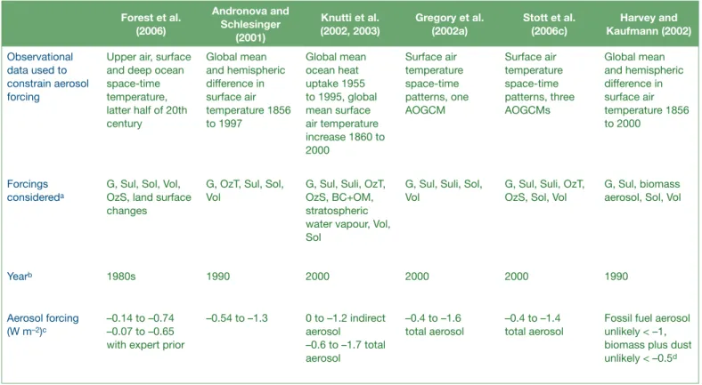
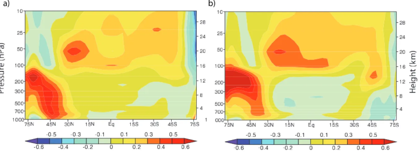
The ability to distinguish between climate responses to different external forcing factors in observations depends on the extent to which those responses are distinct (see, e.g., Section 9.4.1.4 and Appendix 9.A). Figure 9.1 illustrates the zonal average temperature response in the PCM model (see Table 8.1 for model details) to several different forcing agents over the last 100 years, while Figure 9.2 illustrates the zonal average temperature response in the Commonwealth Scientifi c and Industrial Research Organisation (CSIRO) atmospheric model (when coupled to a simple mixed layer ocean model) to fossil fuel black carbon and organic matter, and to the combined effect of these forcings together with biomass burning aerosols (Penner et al., 2007). These fi gures indicate that the modelled vertical and zonal average signature of the temperature response should depend on the forcings. The major features shown in Figure 9.1 are robust to using different climate models. On the other hand, the response to black carbon forcing has not been widely examined and therefore the features in Figure 9.2 may be model dependent. Nevertheless, the response to black carbon forcings appears to be small.

Greenhouse gas forcing is expected to produce warming in the troposphere, cooling in the stratosphere, and, for transient simulations, somewhat more warming near the surface in the NH due to its larger land fraction, which has a shorter surface response time to the warming than do ocean regions (Figure 9.1c). The spatial pattern of the transient surface temperature response to greenhouse gas forcing also typically exhibits a land-sea pattern of stronger warming over land, for the same reason (e.g., Cubasch et al., 2001). Sulphate aerosol forcing results in cooling throughout most of the globe, with greater cooling in the NH due to its higher aerosol loading (Figure 9.1e; see Chapter 2), thereby partially offsetting the greater NH greenhouse-gas induced warming. The combined effect of tropospheric and stratospheric ozone forcing (Figure 9.1d) is expected to warm the troposphere, due to increases in tropospheric ozone, and cool the stratosphere, particularly at high latitudes where stratospheric ozone loss has been greatest. Greenhouse gas forcing is also expected to change the hydrological cycle worldwide, leading to disproportionately greater increases in heavy precipitation (Chapter 10 and Section 9.5.4), while aerosol forcing can infl uence rainfall regionally (Section 9.5.4).

The simulated responses to natural forcing are distinct from those due to the anthropogenic forcings described above. Solar forcing results in a general warming of the atmosphere (Figure 9.1a) with a pattern of surface warming that is similar to that expected from greenhouse gas warming, but in contrast to the response to greenhouse warming, the simulated solar-forced warming extends throughout the atmosphere (see, e.g., Cubasch

et al., 1997). A number of independent analyses have identifi ed tropospheric changes that appear to be associated with the solar cycle (van Loon and Shea, 2000; Gleisner and Thejll, 2003; Haigh, 2003; White et al., 2003; Coughlin and Tung, 2004; Labitzke, 2004; Crooks and Gray, 2005), suggesting an overall warmer and moister troposphere during solar maximum. The peak-to-trough amplitude of the response to the solar cycle globally is estimated to be approximately 0.1°C near the surface. Such variations over the 11-year solar cycle make it is necessary to use several decades of data in detection and attribution studies. The solar cycle also affects atmospheric ozone concentrations with possible impacts on temperatures and winds in the stratosphere, and has been hypothesised to infl uence clouds through cosmic rays (Section 2.7.1.3). Note that there is substantial uncertainty in the identifi cation of climate response to solar cycle variations because the satellite period is short relative to the solar cycle length, and because the response is diffi cult to separate from internal climate variations and the response to volcanic eruptions (Gray et al., 2005).

Volcanic sulphur dioxide (SO₂) emissions ejected into the stratosphere form sulphate aerosols and lead to a forcing that causes a surface and tropospheric cooling and a stratospheric warming that peak several months after a volcanic eruption and last for several years. Volcanic forcing also likely leads to a response in the atmospheric circulation in boreal winter (discussed below) and a reduction in land precipitation (Robock and Liu, 1994; Broccoli et al., 2003; Gillett et al., 2004b). The response to volcanic forcing causes a net cooling over the 20th century because of variations in the frequency and intensity of volcanic eruptions. This results in stronger volcanic forcing towards the end of the 20th century than early in the 20th century. In the PCM, this increase results in a small warming in the lower stratosphere and near the surface at high latitudes, with cooling elsewhere (Figure 9.1b).

The net effect of all forcings combined is a pattern of NH temperature change near the surface that is dominated by the positive forcings (primarily greenhouse gases), and cooling in the stratosphere that results predominantly from greenhouse gas and stratospheric ozone forcing (Figure 9.1f). Results obtained with the CSIRO model (Figure 9.2) suggest that black carbon, organic matter and biomass aerosols would slightly enhance the NH warming shown in Figure 9.1f. On the other hand, indirect aerosol forcing from fossil fuel aerosols may be larger than the direct effects that are represented in the CSIRO and PCM models, in which case the NH warming could be somewhat diminished. Also, while land use change may cause substantial forcing regionally and seasonally, its forcing and response are expected to have only a small impact at large spatial scales (Sections 9.3.3.3 and 7.2.2; Figures 2.20 and 2.23).

(13)

Figure 9.1. Zonal mean atmospheric temperature change from 1890 to 1999 (°C per century) as simulated by the PCM model from (a) solar forcing, (b) volcanoes, (c) well-mixed greenhouse gases, (d) tropospheric and stratospheric ozone changes, (e) direct sulphate aerosol forcing and (f) the sum of all forcings. Plot is from 1,000 hPa to 10 hPa (shown on left scale) and from 0 km to 30 km (shown on right). See Appendix 9.C for additional information. Based on Santer et al. (2003a).

(14)

tend to enhance the high-latitude response of both a positive forcing, such as that of CO₂, and a negative forcing such as that of sulphate aerosol (e.g., Mitchell et al., 2001; Rotstayn and Penner, 2001). Cloud feedbacks can affect both the spatial signature of the response to a given forcing and the sign of the change in temperature relative to the sign of the radiative forcing (Section 8.6). Heating by black carbon, for example, can decrease cloudiness (Ackerman et al., 2000). If the black carbon is near the surface, it may increase surface temperatures, while at higher altitudes it may reduce surface temperatures (Hansen et al., 1997; Penner et al., 2003). Feedbacks can also lead to differences in the response of different models to a given forcing agent, since the spatial response of a climate model to forcing depends on its representation of these feedbacks and processes. Additional factors that affect the spatial pattern of response include differences in thermal inertia between land and sea areas, and the lifetimes of the various forcing agents. Shorter-lived agents, such as aerosols, tend to have a more distinct spatial pattern of forcing, and can therefore be expected to have some locally distinct response features.

The pattern of response to a radiative forcing can also be altered quite substantially if the atmospheric circulation is affected by the forcing. Modelling studies and data comparisons suggest that volcanic aerosols (e.g., Kirchner et al., 1999; Shindell et al., 1999; Yang and Schlesinger, 2001; Stenchikov et al., 2006) and greenhouse gas changes (e.g., Fyfe et al., 1999; Shindell et al., 1999; Rauthe et al., 2004) can alter the North Atlantic Oscillation (NAO) or the Northern Annular Mode (NAM). For example, volcanic eruptions, with the exception of high-latitude eruptions, are often followed by a positive phase of the NAM or NAO (e.g., Stenchikov et al.,

2006) leading to Eurasian winter warming that may reduce the overall cooling effect of volcanic eruptions on annual averages, particularly over Eurasia (Perlwitz and Graf, 2001; Stenchikov et al., 2002; Shindell et al., 2003; Stenchikov et al., 2004; Oman et al., 2005; Rind et al., 2005a; Miller et al., 2006; Stenchikov et al., 2006). In contrast, NAM or NAO responses to solar forcing vary between studies, some indicating a response, perhaps with dependence of the response on season or other conditions, and some fi nding no changes (Shindell et al., 2001a,b; Ruzmaikin and Feynman, 2002; Tourpali et al., 2003; Egorova et al., 2004; Palmer et al., 2004; Stendel et al., 2006; see also review in Gray et al., 2005).

In addition to the spatial pattern, the temporal evolution of the different forcings (Figure 2.23) generally helps to distinguish between the responses to different forcings. For example, Santer et al. (1996b,c) point out that a temporal pattern in the hemispheric temperature contrast would be expected in the second half of the 20th

century with the SH warming more than the NH for the fi rst two decades of this period and the NH subsequently warming more than the SH, as a result of changes in the relative strengths of the greenhouse gas and aerosol forcings. However, it should be noted that the integrating effect of the oceans (Hasselmann, 1976) results in climate responses that are more similar in time between different forcings than the forcings are to each other, and that there are substantial uncertainties in the evolution of the hemispheric temperature contrasts associated with sulphate aerosol forcing.

9.2.2.2 Aerosol Scattering and Cloud Feedback in Models and Observations

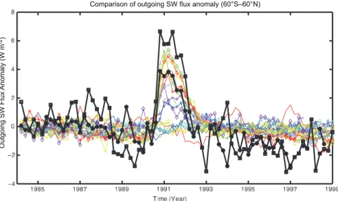
One line of observational evidence that refl ective aerosol forcing has been changing over time comes from satellite observations of changes in top-of-atmosphere outgoing shortwave radiation fl ux. Increases in the outgoing shortwave radiation fl ux can be caused by increases in refl ecting aerosols, increases in clouds or a change in the vertical distribution of clouds and water vapour, or increases in surface albedo. Increases in aerosols and clouds can cause decreases in surface radiation fl uxes and decreases in surface warming. There has been continuing interest in this possibility (Gilgen et al., 1998; Stanhill and Cohen, 2001; Liepert, 2002). Sometimes called ‘global dimming’, this phenomena has reversed since about 1990 (Pinker et al., 2005; Wielicki et al., 2005; Wild et al., 2005; Section 3.4.3), but over the entire period from 1984 to 2001, surface solar radiation has increased by about 0.16 W m–2_yr–1 on average (Pinker et al., 2005). Figure 9.3 shows the

(15)

atmosphere outgoing shortwave radiation fl ux anomalies from the MMD at PCMDI, compared to that measured by the Earth Radiation Budget Satellite (ERBS; Wong et al., 2006) and inferred from International Satellite Cloud Climatology Project (ISCCP) fl ux data (FD) (Zhang et al., 2004). The downward trend in outgoing solar radiation is consistent with the long-term upward trend in surface radiation found by Pinker et al. (2005). The effect of the eruption of Mt. Pinatubo in 1991 results in an increase in the outgoing shortwave radiation

fl ux (and a corresponding dimming at the surface) and its effect has been included in most (but not all) models in the MMD. The ISCCP fl ux anomaly for the Mt. Pinatubo signal is almost 2 W m–2_{larger than that for ERBS, possibly due to} the aliasing of the stratospheric aerosol signal into the ISCCP cloud properties. Overall, the trends from the ISCCP FD (–0.18 with 95% confi dence limits of ±0.11 W m–2_yr–1_{) and the} ERBS data (–0.13 ± 0.08 W m–2_yr–1_{) from 1984 to 1999 are not} signifi cantly different from each other at the 5% signifi cance level, and are in even better agreement if only tropical latitudes are considered (Wong et al., 2006). These observations suggest an overall decrease in aerosols and/or clouds, while estimates of changes in cloudiness are uncertain (see Section 3.4.3). The model-predicted trends are also negative over this time period, but are smaller in most models than in the ERBS observations (which are considered more accurate than the ISCCP FD). Wielicki et al. (2002) explain the observed downward trend by decreases in cloudiness, which are not well represented in the models on these decadal time scales (Chen et al., 2002; Wielicki et al., 2002).

9.2.2.3 Uncertainty in the Spatial Pattern of Response

Most detection methods identify the magnitude of the space-time patterns of response to forcing (sometimes called ‘fi ngerprints’) that provide the best fi t to the observations. The fi ngerprints are typically estimated from ensembles of climate model simulations forced with reconstructions of past forcing. Using different forcing reconstructions and climate models in such studies provides some indication of forcing and model uncertainty. However, few studies have examined how uncertainties in the spatial pattern of forcing explicitly contribute to uncertainties in the spatial pattern of the response. For short-lived components, uncertainties in the spatial pattern of forcing are related to uncertainties in emissions patterns, uncertainties in the transport within the climate model or chemical transport model and, especially for aerosols, uncertainties in the representation of relative humidities or clouds. These uncertainties affect the spatial pattern of the forcing. For example, the ratio of the SH to NH indirect aerosol forcing associated with the total aerosol forcing ranges from –0.12 to 0.63 (best guess 0.29) in different studies, and that between ocean and land forcing ranges from 0.03 to 1.85 (see Figure 7.21; Rotstayn and Penner, 2001; Chuang et al., 2002; Kristjansson, 2002; Lohmann and Lesins, 2002; Menon et al., 2002a; Rotstayn and Liu, 2003; Lohmann and Feichter, 2005).

9.2.2.4 Uncertainty in the Temporal Pattern of Response

Climate model studies have also not systematically explored the effect of uncertainties in the temporal evolution of forcings. These uncertainties depend mainly on the uncertainty in the spatio-temporal expression of emissions, and, for some forcings, fundamental understanding of the possible change over time.

The increasing forcing by greenhouse gases is relatively well known. In addition, the global temporal history of SO2 emissions, which have a larger overall forcing than the other short-lived aerosol components, is quite well constrained. Seven different reconstructions of the temporal history of global anthropogenic sulphur emissions up to 1990 have a relative standard deviation of less than 20% between 1890 and 1990, with better agreement in more recent years. This robust temporal history increases confi dence in results from detection and attribution studies that attempt to separate the effects of sulphate aerosol and greenhouse gas forcing (Section 9.4.1).

In contrast, there are large uncertainties related to the anthropogenic emissions of other short-lived compounds and their effects on forcing. For example, estimates of historical emissions from fossil fuel combustion do not account for changes in emission factors (the ratio of the emitted gas or aerosol to the fuel burned) of short-lived species associated with concerns over urban air pollution (e.g., van Aardenne et al., 2001). Changes in these emission factors would have slowed the emissions of nitrogen oxides as well as carbon monoxide after about 1970 and slowed the accompanying increase in tropospheric ozone compared to that represented by a single emission factor for fossil fuel use. In addition, changes in the height of SO2 emissions associated with the implementation of tall stacks would have changed the lifetime of sulphate aerosols and the relationship between emissions and effects. Another example relates to the emissions of black carbon associated with the burning of fossil fuels. The spatial and temporal emissions of black carbon by continent reconstructed by Ito and Penner (2005) are signifi cantly different from those reconstructed using the methodology of Novakov et al. (2003). For example, the emissions in Asia grow signifi cantly faster in the inventory based on Novakov et al. (2003) compared to those based on Ito and Penner (2005). In addition, before 1988 the growth in emissions in Eastern Europe using the Ito and Penner (2005) inventory is faster than the growth based on the methodology of Novakov et al. (2003). Such spatial and temporal uncertainties will contribute to both spatial and temporal uncertainties in the net forcing and to spatial and temporal uncertainties in the distribution of forcing and response.

Understanding and Attributing Climate Change

9