Controlling regional monopolies in the natural gas industry: the role of transport capacity

Controlling regional monopolies in the natural gas

industry: The role of transport capacity

F. GASMI

Toulouse School of Economics (ARQADE & IDEI)

and J.D. OVIEDO Universidad del Rosario

Abstract

This paper analyzes some optimal fiscal, pricing, and capacity investment policies for controlling regional monopoly power in the natural gas industry. By letting the set of control instruments available to the social planner vary, we provide a characterization of the technological and demand conditions under which “excess” capacity in the transport network arises in response to the loss of the two other control instruments, namely, transfers and pricing. Hence, the analysis yields some insights on an economy’s incentives to in-vest in infrastructures for the purpose of integrating geographically isolated markets.

JEL-code: L51, L95

Key words: Market power, Natural gas, Excess transport capacity.

October 2012

†_{Corresponding author: J.D. Oviedo, Universidad del Rosario, Bogota, Colombia,}

1

Introduction

Following the US and the UK that reformed their natural gas industries in the late 70s and the 80s respectively, the EU has launched in the late 90s structural policies for enhancing gas-to-gas competition with the objective of complete liberalization of the market by 2007. More recently, EU Mem-ber States have been heavily investing in the development of their pipeline networks and Liquefied Natural Gas (LNG) liners. Such investments can be seen as driven by the need to anticipate growth of demand and import de-pendency. Indeed, gas penetration in energy consumption across activities in Europe has increased from less than 10% in the 70s to a current level of about 25% with an external dependency around 50%.1 Still, some observers have come to wonder whether such large-scale investments in capacity ex-pansion are all that needed (Junola, 2003) and can be justified only on demand pressure and security of supply grounds. In this paper, we focus on the industrial organization role of transport capacity investments, namely, on their impact on market structure and the exercise of market power in the natural gas industry.

Since bringing the benefits of competition to consumers is a stated goal of the EU gas directive adopted in 1998 and amended in 2003 and given the high concentration of both commodity supply and transport in the EU region, it makes sense to investigate the role of network investments in the liberalization process. An issue that is particularly important for the EU is the nature of policies that should accompany this liberalization process and their effectiveness in mitigating the economic distortions that would result from a competitive market structure which is expected to be at best imperfect in the foreseeable future. A widely used transitory instrument for fostering gas-to-gas competition that has had varying degrees of success throughout the countries of the Union is gas release.2 _{This paper considers} fiscal, pricing, and investment in capacity policies for improving market

1_{Algeria, Norway, and Russia are the main suppliers for Europe.}

2_{Chaton et al. (2008) have analyzed gas release as a short term instrument with the}

efficiency and focuses on the role of transport network expansion.3

The relationship between network capacity and market structure in en-ergy markets has attracted the attention of both empirical and theoretical economists. For the case of the US gas industry, a large empirical literature has examined the impact of investments in sub-network interconnection on the degree of market integration and the level of competition (see, among others, Doane and Spulber, 1994, and De Vany and Walls, 1994). From a more theoretical perspective, in electricity, a stream of the literature has examined the direct impact of transmission capacity on local market power (see, e.g., Borenstein et al., 2000 and L´eautier, 2001) reaching the conclu-sion that transmisconclu-sion link expanconclu-sion is effective for promoting competition. Building on a framework developed in Cremer et al. (2003), Cremer and Laffont (2002) argue that countering local market power in the natural gas industry might necessitate building excess transport capacity. McAfee and Reny (2007) also highlight the role of excess transport capacity in the de-termination of market power in natural gas transportation markets. The purpose of this paper is to further investigate the relationship between net-work size and regional market power.

At this initial stage of our investigation, the theoretical framework on which our analysis rests assumes away information problems.4 We consider a social planner who possesses complete information on demand and technol-ogy and controls the market power of an incumbent monopoly in a regional commodity gas market with a set of three instruments: transfers between consumers and the firm, pricing of the gas commodity, and investments in the capacity of the transport network. Starting from a situation where this whole set of control instruments is available to the social planner and reducing this set by first removing transfers and then transfers and price, should make the social planner rely more intensively on transport capacity

3_{Note that the problem of market power due to geographic isolation, which is the}

subject of this paper, is common in economics. Breaking up the isolation by investing in means of communications is obviously a solution but how much to invest is the relevant question.

4_{Gasmi and Oviedo (2010) use a similar complete information framework to show how}

in order to counter monopoly power. Hence, fulfilling this objective with-out the ability to use transfers and control price can be expected to require a strictly higher level of transport capacity. Giving a characterization of the technological and demand conditions under which this “excess capacity hypothesis” holds is the main motivation of this paper. Our analytical strat-egy consists first in characterizing the optimal policies under the alternative control schemes, i.e., the optimal levels of the instruments used in each con-trol regime, and then examining the relative levels of capacity these policies prescribe. These comparisons allow us to assess the extent to which trans-port capacity compensates for the lack/loss of the two other instruments of market power control. This analysis of optimal dimensioning of networks thus yields some insights on society’s incentives to invest in infrastructure in increasingly liberalized markets.

The plan of the paper is as follows. The next section describes the model of the industry configuration we consider and its basic theoretical ingredi-ents. Sections 3, 4, and 5 characterize the optimal policies under three control schemes. These schemes are, respectively, one that lets the social planner have the largest set of instruments of market power control, namely, transfers, price, and capacity, one in which transfers are not allowed, and one in which the social planner controls only the capacity of the transport net-work. Section 6 focuses on the capacity variable and presents results on the excess capacity hypothesis. We summarize our main findings, discuss some of their policy implications, and give some directions for further research in the conclusion. Formal proofs and some illustrations of the optimal policies using some specific functional forms for the demand and cost functions are given in the appendix.

2

Industry configuration

Fm >0 is fixed cost.5 Gas is also supplied at marginal cost c in a

competi-tive market, marketCp, which is geographically distinct from marketM but

could be linked to it if a pipeline of capacityK is built at cost C(K), where

C(_·) is increasing convex, C′_{(0) = 0, and C}′′_{(0)> 0. Figure 1 below gives}

a schematic representation of this industry configuration. We assume that the regional monopoly’s marginal cost is greater than marginal cost of gas produced in market Cp, i.e., θ > c.6 Gas produced under competitive

con-ditions in marketCp and imported into the regional commodity gas market M should counter the exercise of market power by firm min this market.

s s

Cp

c

M

Cm(θ, qm) =θqm+Fm

K,C(K)

✲

Figure 1: Industry configuration

Our analysis rests on the presumption that the very reason for a social planner to support a policy of building a transport line that links these two markets is to allow imports of gas from marketCp into market M that

would bring consumers in this latter market the benefits of competition. LettingQM(·) represent these consumers’ demand function, assumed to be

downward-slopping and concave, if a quantity of gas corresponding to full capacity of the pipeline K is shipped from the competitive market into the regional market, firm m remains a monopoly on the residual demand

QM(pM)−K, wherepM is price. We assume that the social planner knows

the demand and cost functions QM(·) and Cm(·) and seeks to determine

policies that would restrain the firm from exerting its monopoly power in the regional market. An obvious yet important policy would be to interconnect this regional market and the competitive market Cp with a pipeline. The

question then is what the optimal size of this pipeline should be and the answer to this question should clearly depend on what other instruments the social planner has to mitigate the monopoly power of firmm.

5_{We assume that the fixed costF}

mis bounded and later provide a technical justification for this assumption. Even though shutting down the firm is sometimes prescribed by the optimal policies considered in this paper, the financing of this fixed cost is always taken into account.

6_{This assumption reflects the standard productive inefficiency consequence of market}

As is common in public economics, we assume that this public inter-vention takes place under second-best conditions in which public funds are raised through distortionary taxes at a (social) cost of λ >0. Also, in the industry configuration considered in the paper we focus only on demand in the regional market and any pricing policy implemented in this market wouldn’t affect welfare in the competitive market where price is at the first-best level (marginal cost c). Hence, without loss of generality, we do not include welfare achieved in this competitive market into the analysis.7

We start from a situation where the social planner has the ability to control the regional monopoly by means of three instruments, namely, (pos-sibly two-way) transfers between consumers and the firm, price, transport capacity of the network, and hence monopoly output. We then restrict the set of available control instruments. We first consider the case where the social planner may not use transfers when setting the price and capacity levels. Then, we examine the situation where in addition to the fact that transfers are not allowed, the social planner can only influence the gas com-modity price in the regional market through transport capacity that affects the residual demand of the monopoly.

3

Controlling the regional monopoly with

transfers, price, and transport capacity

In this section, we assume that the social planner may use public funds to make transfers between consumers and the firm. These funds are raised through taxation that generates welfare losses so that a monetary transfer to the firmT costs society (1 +λ)T whereλis the cost of public funds. Let

S(_·) represent gross surplus of consumers in marketM. Total supply of gas

QM(pM) in this market, composed of K units imported from the

competi-tive market and qm units produced locally by firm m, brings taxpayers an

7_{Another factor that is excluded from the analysis without affecting the main}

aggregate (net) welfareV given by

V = _{S(QM(pM))−pMQM(pM)}

+_{(1 +λ) [(pM −c)K−C(K)]} − {(1 +λ)T} (1)

This taxpayers’ welfare comprises three parts: the net surplus of consumers in the regional market M, the social valuation of profits generated by the

K units of gas imported from the competitive market, and the social cost of the transfer T made to the firm. The welfare of firm m is measured by its utility U that sums its profits from sales and the transfer it receives:

U =_{(pM −θ) [QM(pM)−K]−Fm}+T (2)

When controlling the regional monopoly, the social planner has to ac-count for the participation constraint of the firm and the constraint of non-negativity of its output:8

U _≥0 (3)

qm=QM(pM)−K ≥0 (4)

The utilitarian social welfare functionW is the sum of taxpayers’ welfareV

and firm’s utility U. Substituting for V from (1) and for T from (2) yields social welfare

W = _{S(QM(pM)) +λpMQM(pM)

−(1 +λ) [θ(QM(pM)−K) +cK+C(K) +Fm]} −λU (5)

as the social valuation of total production minus its social cost, minus the social opportunity cost of the firm’s utility. From this expression of social welfare we see that reducing the monopoly’s utility, its “rent,” is socially desirable for, as can be seen from (2), this utility includes a transfer of public funds collected through distortive taxation. Similarly, we see from (5) that the social valuation of total production explicitly includes the fiscal value of the revenues that it generates λpMQM(pM).9

8_{The output nonnegativity constraint needs to be taken into account here because}

transfersT (here unconstrained in sign and magnitude) can be used to finance any fixed cost that wouldn’t be recovered through revenues from gas.

9_{Indeed, these revenues allow the government to rely less on public funds raised through}

With transfers, monopoly output, and capacity as instruments of control, the social planner’s program consists in maximizing social welfareW given by (5) with respect to pM, K, and U, under the firm’s participation and

output nonnegativity constraints, respectively (3) and (4).10 Lettingφand

ν denote the Lagrange multipliers associated with these two constraints respectively, and using the fact that ∂S(QM)/∂QM = pM, the following

first-order conditions obtain:11

λQM+ (1 +λ) (pM−θ)Q′M +νQ′M = 0 (6)

(1 +λ) [(θ₋c)₋C′_{(K)]−ν= 0 (7)}

−(λ₋φ) = 0 (8)

φU = 0 (9)

ν[QM −K] = 0 (10)

From (8) and (9), we immediately see that the participation constraint is binding, i.e.,U = 0 and, indeed, transfers allow the social planner to totally extract (finance) the firm’s profit (deficit). Letting ε(QM) designate the

price-elasticity of demand in market M, the first-order conditions (6)-(10) allow us to state the following proposition:12

Proposition 1 When price (or equivalently output) and capacity are both

controlled by the social planner and, in addition, the latter can use public funds to make transfers between consumers and the firm, one of two following policies (K, pM, ν) arises:

(i) The policy (0< K < QM, pM > θ, ν= 0) in which the local monopoly

meets part of the market demand and price and capacity satisfy

pM −θ

pM

= pM −(c+C′(K))

pM

= λ 1 +λ

1

ε(QM)

(11)

(1 +λ)C′_{(K) = (1 +λ)(θ−c) (12)}

10_{Note that as long as the social planner controls monopoly output and transport}

ca-pacity, he totally controls price in marketM.

11_{To minimize notation and where it doesn’t lead to any ambiguity, the arguments of}

some of the demand and cost functions will be dropped in the presentation.

12_{An illustration of the approach used to solve the social planner program is provided}

(ii) The policy (K =QM, pM > c, ν > 0) in which the local monopoly is

shut down, market demand is entirely met through imports, and the markup of the import activity is given by

pM −(c+C′(QM))

pM

= λ 1 +λ

1

ε(QM)

(13)

Under policy (i), the condition (θ₋c) < C′_{(QM) holds, i.e., the firm’s}

marginal cost, θ, is smaller than the marginal cost of imports when the latter meet the entire market demand, c+C′_{(QM). Under policy (ii) the}

reverse is true.

Note that, thanks to the availability of transfers, the policies described in Proposition 1 are not responsive to the value of the fixed cost,Fm. Under

both policies we see from equations (11) and (13) that pricing obeys a Ram-sey principle according to which the price markup is inversely proportional to the price-elasticity of demand in the regional market.13 When ν = 0, i.e., when the local monopoly is active, it is indeed optimal to let it apply a markup (see (11)) since public funds are costly and the social planner can use transfers to capture this markup. As to capacity, it is set such that the social marginal cost of imports, (1 +λ)[c+C′_{(K)], is equal to the social}

marginal cost of local production, (1 +λ)θ, a relationship that can be seen from (12). When ν >0, i.e., when the firm is shut down, its fixed cost is financed through transfers and there is still a markup but now the relevant marginal cost is that of imported gas (see (13)).

4

Controlling the regional monopoly with price

and capacity only

We now assume that the social planner can still set the transport capacity and the firm’s output level, and hence fully controls price in marketM, but transfers between consumers and the firm are no longer permitted. Social

13_{Note that here the coefficient of proportionality is a function of λ and hence, in}

welfareW is expressed as

W = _{S(QM(pM))−pMQM(pM)}

+_{(1 +λ) [(pM −c)K−C(K)]}

+_{(pM −θ) [QM(pM)−K]−Fm} (14)

that is, as the sum of the net consumer surplus, the social value of the profits generated by the K units imported from the competitive market, and the profits of the firm that now cannot be transferred to consumers. Gathering terms, we obtain

W = S(QM(pM)) +λpMK

−[θ(QM(pM)−K) +Fm]−(1 +λ) [cK+C(K)] (15)

Cross-examining (5) and (15), we see that as now transfers are not allowed, the social planner assigns a fiscal valueλpMKonly to the revenues generated

by the K units shipped from the competitive market Cp into the regional

marketM.

The social planner maximizes social welfare given by (15) with respect to price and capacity, under the participation constraint (nonnegativity of profits), that now does not include transfers, and the firm’s output nonneg-ativity constraint

Πm = (pM −θ) [QM(pM)−K]−Fm ≥0 (16)

qm=QM(pM)−K ≥0 (17)

Given that transfers are not allowed, it makes sense for us to consider only the policies with pM > θ when the firm is active, which is always the case

from (16) since we assumeFm>0.14 Hence, from now on, we focus on the

set defined by the participation constraint (16) hereafter referred to as the

participation set.

Letting φ denote the Lagrange multiplier associated with the partici-pation constraint, the system of first-order conditions that characterize the

14_{When there is no fixed cost, i.e.,F}

optimal policy is given by

λK+ (pM −θ)Q′M+φ[(pM−θ)Q′M + (QM −K)] = 0 (18)

(1 +λ) [(θ₋c)₋C′_{(K)] + (λ−φ) (p}

M−θ) = 0 (19)

φ[(pM −θ) (QM−K)−Fm] = 0 (20)

(pM −θ) (QM −K)−Fm ≥0 (21)

To rule out the possibility of havingK <0 we assume that the fixed cost is bounded so that

Fm ≤ −

λQ2_M +h(1 +λ)(θ₋c)Q′

M +

√

ΓiQM

2(1 +λ)Q′ M

(22)

where Γ_≡[λQM + (1 +λ)(θ−c)Q′M]

2

−4(1 +λ)2_(θ−c)Q

MQ′M.15

The next proposition characterizes the alternative pricing and transport capacity policies associated with this two-instrument control scheme.

Proposition 2 When price (or equivalently output) and capacity are both

controlled by the social planner but the latter cannot use public funds to make transfers between consumers and the firm, there are two exclusive candidate policies (K, pM, φ) with one of them having two possible forms:

15_{This upper-bound is obtained as follows. WhenF}

m >0, we look for the conditions characterizing a policy of the type (0, pM > θ, φ > 0). Substituting for K = 0 in the system of first-order conditions (18)-(20), we see that such a policy is defined by

φ=λ+(1 +λ)(θ−c)QM

Fm

and φQM+

(1 +φ)FmQ′M

QM

= 0.

Solving forFm, yields the right-hand side term of the inequality (22). It is easy to see that anyFm smaller than this term will indeed yieldK >0. Moreover, it can be shown that (22) impliesFm≤ −Q2M/Q′M, which is a condition that ensures that the participation set be nonempty for nonnegative values ofK. The latter condition is derived as follows. For the participation set to be nonempty forK≥0 it suffices that the largestK that makes the participation constraint binding be nonnegative. Such aK is found by solving the following program:

max pM,K K

s.t. (pM−θ) [QM(pM)−K]−Fm= 0

K≥0

It is then easy to show that such a capacity level satisfies [Q′

(i) The policy (K = 0, pM > θ, φ > λ) which consists in building no

capacity and letting the local monopoly earn a markup that makes it just break even:

pM −θ

pM

= φ 1 +φ

1

ε(QM)

(23)

(ii) The policy (0 < K < QM, pM > θ, φ ≥ 0) which prescribes building

capacity and setting price above marginal cost. This policy takes one of the two following forms:

(a) The policy (0< K < QM, pM > θ, φ= 0), characterized by

pM −θ

pM

= λK

QM

1

ε(QM)

(24)

pM −(c+C′(K))

pM

= λ 1 +λ

K

QM

1

ε(QM)

(25)

(1 +λ)C′_{(K) = (1 +λ)(θ−c)−λ}2 K

Q′ M

(26)

(b) The policy (0 < K < QM, pM > θ, φ > 0) in which the pricing

and capacity building rule are characterized by

pM−θ

pM

=

λK +φ(QM −K)

(1 +φ)QM

1

ε(QM)

(27)

pM −(c+C′(K))

pM

=

λK +φ(QM −K)

(1 +λ)QM

1

ε(QM)

(28)

(1 +λ)C′_{(K) = (1 +λ)(θ−c) +} Υ

(QM−K)

(29)

where Υ _≡ m_{Πm ×}[λQM(QM−K) + (1 +λ)Q′MFm] > 0, and

m_Πm = pM−θ

(QM−K)+(pM−θ)Q′

M =

Fm

Q′

MFm+(QM−K)2

Under policy (i) the fixed cost hits its bound, i.e., the condition (22) is satisfied with equality. Whenever (22) is satisfied with strict inequality only policies of type (ii) may arise. Policy (ii-a) corresponds to the case where the marginal cost of the regional monopoly, θ, equals the “net” social marginal cost of imports, (1 +λ)[c+C′_{(K)]−λpM, i.e., Q}′

M h

C′′_(K)−C′(K) K

i − λK

Q′

MQ

′′

cost, i.e., Fm < −λK(QM_Q′−K)

M . Policy (ii-b) corresponds to the case where either of these inequalities is reversed.

From Proposition 2, we see that when the solution of the constrained welfare maximization program allows the monopoly to earn positive profits (case where φ = 0), i.e., under policy (ii-a), it makes a markup which is inversely related to the elasticity of demand and increases with the share of imports in the total consumption of gas in the regional market. The reason for this latter result is that the social marginal valuation of capacity increases with price. As to the markup made on imports, it is increasing with the share of these imports in total demand but it is less sensitive to it than the firm’s markup. From the capacity building rule under this policy, we see that the social cost of the marginal unit of gas shipped from the competitive market, (1 +λ)[c+C′_{(K)], net of the fiscal revenue of this imported gas}

unit, λpM, equals the social cost of having this unit produced by the local

monopoly,θ.

When it is optimal to let the local monopoly active and just break even

((qm>0,K >0, andφ >0)), i.e., under policy (ii-b), the markup made by

the monopoly is again inversely related to the regional market demand elas-ticity. However, the proportionality term is the ratio of the fiscal valuation of the revenues from imports,λpMK, plus the valuation the planner assigns

to the fact that revenues made by the firm help to relax the participation constraint,φpMqm, to the social valuation of the aggregate revenues in the

regional market in the case where these revenues were exclusively generated by the firm, (1 +φ)pMQM. The markup from imports has a similar

struc-ture but the denominator of the proportionality term is the social valuation of aggregate revenues in the case where total demand is met by imports, (1 +λ)pMQM.16 Under this zero-profit policy, optimal capacity makes the

“net” social cost of the marginal unit of gas shipped from the competitive market, (1 +λ)[c+C′_(K)]−λp

M, just equal to the social cost of having this

unit produced by the local monopoly,θ, net of the value the planner assigns to the contribution of this unit to the relaxation of the firm’s participation

16_{This interpretation is obtained after multiplying the right-hand side expressions of}

constraint, φ(pM −θ). Indeed, these profits can no longer be collected by

the planner who now lacks the instrument (transfers) that would allow him to do so.

Finally, under policy (i) the fixed cost is so high that it is optimal to let the regional monopoly cover full market demand and hence no capacity is built (K = 0).

5

Controlling the regional monopoly with

transport capacity only

We now assume that the social planner lacks an additional instrument of con-trol, namely, setting the monopoly’s level of output, and hence he can only partially affect price in marketM through the residual demand. Transport capacity is therefore the only instrument left to him to counter the exer-cise of local market power by the firm in this market. In practice though, we model this case as if the social planner continues to set the price level, but now this price has to fall within a profit-maximizing-constrained set of values. Let us be more specific.

For a given volume of gasK imported from the competitive market, the firm remains a monopoly in its local commodity gas market on the residual demand QM(pM)−K. Given this demand, the firm sets price so as to

maximize its profit Πm given by

Πm = (pM −θ) [QM(pM)−K]−Fm (30)

The first-order condition of this profit-maximization problem is

(pM −θ)Q′M+QM −K = 0 (31)

while the second-order condition that ensures that we are indeed at a max-imum is Ω_≡(pM −θ)Q′′_M + 2Q′_M <0.

section which we restate here:

W = S(QM(pM)) +λpMK

−θ(QM(pM)−K)−(1 +λ) [cK+C(K)]−Fm (32)

The program of the social planner consists in maximizing social welfare given by (32) with respect topM andK, under the regional monopoly participation

constraint, Πm ≥ 0, where Πm is given by (30), its output nonnegativity

constraint,qm≥0, and its profit-maximization constraint (31).17 As in the

previous section, let us focus on policies with pM > θ in which case the

firm’s output nonnegativity constraint can be ignored.18 Letting φ and η

designate the Lagrange multipliers associated with the firm’s participation and profit-maximization constraints, respectively, we obtain the following first-order conditions:19

λK+ (pM −θ)Q′M −ηΩ = 0 (33)

(λ₋φ) (pM −θ) + (1 +λ) [(θ−c)−C′(K)] +η= 0 (34)

φ[(pM −θ)(QM −K)−Fm] = 0 (35)

(pM −θ)(QM −K)−Fm ≥0 (36)

(pM −θ)Q′M+QM −K = 0 (37)

The following proposition summarizes the policies characterized by these first-order conditions.

Proposition 3 When capacity is the only instrument controlled by the so-cial planner, it is always built and there are two exclusive candidate policies

(K, pM, φ, η):

17_{Strictly speaking, the second-order condition of the firm’s profit-maximization}

pro-gram should also be taken as a constraint. The standard way to deal with this issue, is to check ex post that this second-order condition is satisfied by the solution of the program.

18_{Indeed, (p}

M−θ)>0 and (31) implyqm≥0. Note that in this case there is no need for a constraint on the size of the marginal cost gap.

19_{The Lagrange multiplier associated with the profit-maximization constraint (31),η, is}

(i) The policy (0< K < QM, pM > θ, φ= 0, η6= 0) characterized by

pM −θ

pM

=

λK₋ηΩ

QM

1

ε(QM)

=

QM −K

QM

1

ε(QM)

(38)

pM −(c+C′(K))

pM

=

λK₋η(Ω₋Q′

M)

(1 +λ)QM

1

ε(QM)

(39)

(1 +λ)C′_{(K) = (1 +λ)(θ−c)−}λ(QM −K)

QM′ −

QM −(1 +λ)K

Ω (40)

where Ω is as defined above.

(ii) The policy (0 < K < QM, pM > θ, φ > 0, η 6= 0)characterized by the

average cost pricing rule

pM−θ

pM

=

QM −K

QM

1

ε(QM)

=

p

−QM′Fm

QM

1

ε(QM)

(41)

pM −(c+C′(K))

pM

=

(1 +φ)[λK₋ηΩ] +ηQ′ M

(1 +λ)QM

1

ε(QM) ,

(42)

K =QM −

p

−QM′Fm (43)

Under policy (i) the marginal cost of the local monopoly θ plus the shadow cost of the firm’s profit maximization constraint, η, equals the “net” social marginal cost of imports, (1 +λ)[c+C′_(K)]−λp

M, and

the resulting firm’s variable profits are larger than the fixed cost, i.e., Fm <−(QM−K)

2

Q′

M . Under policy (ii) this condition holds with equality, i.e.,Fm=−(QM−K)

2

Q′

M .

Proposition 3 says that when the solution allows for positive profits by monopoly (φ = 0), i.e., under policy (i), this firm earns a markup which is proportional to the share of its output in the aggregate demand and inversely related to the elasticity of demand. The size of this markup is larger (smaller) than that under the control scheme where the social planner had total control over pricing, described in section 4, if the shadow cost of the firm’s profit maximization constraint,η, is positive (negative). Optimal capacity is determined by balancing the net social cost of having an extra unit imported from the competitive market, (1+λ)[c+C′_(K)]−λp

the cost of having that unit produced locally by the monopoly, θ, plus the social cost of complying with the profit-maximization constraint, η.

When this mono-instrument control scheme yields no profits for the local monopoly at the optimum (φ >0), i.e., under policy (ii), the firm’s markup is inversely related to the elasticity of demand but increases with the size of the fixed cost. Since in this particular case capacity is used by the social planner as a residual instrument to make the firm just break even, it is decreasing inFm (see (43)).

6

Role of transport capacity

So far, we have characterized optimal policies obtained under three control schemes that are differentiated by the set of control instruments available to the social planner. More specifically, we have considered the benchmark case in which the social planner can use transfers, capacity, and price to mitigate regional monopoly power. Then, we have studied the more realistic cases in which first, transfers are not allowed, second, neither transfers nor price control are possible. By comparing the levels of transport capacity achieved under these three alternative market power control schemes, we now provide a characterization of some conditions that would be interpreted as leading to “excess” capacity in the sense that, under these conditions, optimal policies command systematically higher levels of transport capacity.

For clarity of exposition, we refer to the schemes described in section 3 (control of price and capacity with transfers), 4 (control of price and capacity without transfers), and 5 (control of capacity only) as schemes A,

B, andCrespectively. We study the evolution of network capacity as the set of instruments that the planner uses maximize social welfare gets reduced. Letting KA_{, K}B_{, K}C_{, and p}A

M, pBM, pCM designate the optimal levels of

in order to mitigate regional monopoly power.20

6.1 Excess capacity due to the loss of transfers as a control instrument

When analyzing the impact of the loss of (only) the ability to use transfers between consumers and the firm, the relevant comparison is between schemes

A and B. We express the first-order conditions of the constrained welfare maximization programs under these schemes, (6), (7), and (18), (19) as follows:

∂WA

∂pM

+νA_Q′

M = 0 (44)

∂WA

∂K −ν

A _{= 0 (45)}

∂WB

∂pM

+φB∂Πm

∂pM

= 0 (46)

∂WB

∂K −φ

B_(p

M −θ) = 0 (47)

Examining the left-hand sides of (44), (46), and (45), (47), we see that

∂WB

∂pM

= ∂W

A

∂pM −

λ∂Πm

∂pM

(48)

∂WB

∂K =

∂WA

∂K +λ(pM−θ) (49)

A casual look at (44)-(49) suggests that the (endogenous) shadow cost of the constraint of nonnegativity of the firm’s output, νA, the (endogenous) shadow cost of its participation constraint, φB_{, and the (exogenous) social}

cost of public funds, λ, are going to influence the relative optimal levels of transport capacity. The following proposition formalizes this relationship.

Proposition 4 The loss of (only) transfers as a control instrument has the

following consequences. When the shadow cost of the participation constraint under scheme B, φB, is smaller than the social cost of public funds, λ,

20_{Each pairwise comparison is illustrated by using specific functional forms and}

i.e., (λ₋φB_{)>0, society suffers a net marginal cost from letting the firm}

make positive profits under this scheme and “excess” capacity is needed, i.e.,

KB_{> K}A_.

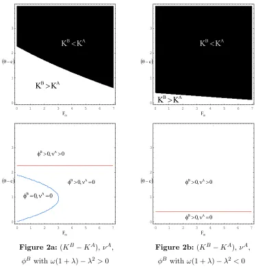
As an illustration of this proposition, Figures 2a and 2b below exhibit the sign of the capacity differential, (KB_−KA_{), and that of ν}A _{and φ}B_{, in}

terms of the marginal cost gap, (θ₋c), and the fixed cost, Fm, assuming

the functional forms given by

QM(pM) =γ−pM, C(K) =

ω

2K

2_{; γ, ω >0, γ > c (50)}

and for the grid of parameters values (λ, ω, γ, c)_{∈ {}(1/3,1/2,10,2),(1/3,1/15,10,2)_}.21

21_{These two sets of parameter values allow us to examine both the case where the}

0 1 2 3 4 5 6 7 0

1 2 3

A B

K

K

_!

A B

K

K

Tc

m F

0 1 2 3 4 5 6 7

0 1 2 3

A B

K

K

_!

A B

K

K

Tc

m F

0 1 2 3 4 5 6 7

0 1 2 3

Tc

m F 0 , 0 A B

Q I

0 , 0 A B

Q ! I

0 , 0 A B

! Q ! I

0 1 2 3 4 5 6 7

0 1 2 3

Tc

m F

0 , 0 A B

Q ! I

0 , 0 A B

! Q ! I

Figure 2a: (KB_−KA_),νA_{, Figure 2b:(K}B_−KA_),νA_,

φB withω(1 +λ)₋λ2 >0 φB with ω(1 +λ)₋λ2<0

Cross-examining the upper and lower parts of Figures 2a and 2b, we see that whenever the solution under scheme B is interior (φB _{= 0), so is}

6.2 Excess capacity due to the loss of price control

Suppose now that the social planner initially has two control instruments, price and capacity, and then looses the ability to set price. In order to analyze the impact of such a reduction in the set of control instruments, the relevant comparison is between schemes B and C. Since the welfare functions of these two schemes are identical and schemeC has an additional constraint (the firm’s profit-maximization constraint), let us express its first-order conditions (33), (34), and (37) as

∂WB

∂pM −

ηCΩ = 0 (51)

∂WB

∂K −φ

C_(p

M −θ) +ηC = 0 (52)

∂Πm

∂pM

= 0 (53)

These first-order conditions give us reasons to expect that the shadow costs of the participation constraint underB and C,φB _{and φ}C_{, and that of the}

profit-maximization constraint underC,ηC, are going to be influential in the determination of the relative size of transport capacity. These expectations are confirmed in the next proposition.

Proposition 5 When price and capacity are first controlled by the social

planner and then the latter looses price control, the impact on network ca-pacity is as follows. When the social marginal cost of letting the firm max-imize profits is positive, i.e., when ηC _{> 0, the lose of price control by the}

social planner entails “excess” capacity, i.e.,KC > KB.

Figures 3a and 3b below show the sign of the capacity differential, (KC₋ KB_{), and that ofφ}B_,φC_{, andη}C _{in terms of the marginal cost gap, (θ−c),}

and the fixed cost, Fm, assuming the functional forms given by (50) and

0 1 2 3 4 5 6 7 0

1 2 3

Tc

m F B C

K

K

_!

0 1 2 3 4 5 6 7

0 1 2 3

Tc

m F B C

K

K

_!

0 1 2 3 4 5 6 7

0 1 2 3

Tc

m F 0 , 0 , 0 C C B ! K ! I ! I 0 , 0 , 0 C C B ! K ! I I 0 , 0 , 0 C C B ! K I I 0 , 0 ,

0 C C

B ! K I ! I 0 , 0 , 0 C C B K ! I ! I 0 , 0 , 0 C C

B_{! I K}

I

0 , 0 , 0 C C B

K I I

0 1 2 3 4 5 6 7

0 1 2 3

Tc

m F 0 , 0 , 0 C C B ! K ! I ! I 0 , 0 , 0 C C B K ! I ! I 0 , 0 , 0 C C B K I ! I

Figure 3a: (KC_−KB_{), φ}B_,φC_{, Figure 3b:(K}C_−KB_{), φ}B_,φC_,

ηC with ω(1 +λ)₋λ2 >0 ηC withω(1 +λ)₋λ2<0

Comparing the upper and lower parts of Figures 3a and 3b, we see that whenever the solution under schemeC yields ηC _{>0, the capacity}

differen-tial is such that KC₋KB >0. With the functional forms (50), condition

Q′ M

h

C′′_(K)−C′(K) K

i −QλK′

MQ

′′

MC′′(K)<0 does not hold and Figure 3b

con-firms the statement in Proposition 2 that wheneverω(1 +λ)₋λ2 _{<0, the} solution underB hasφB_>0.22

22_{This condition represents the inequality (1+λ)Q}′

6.3 Excess capacity due to the loss of both transfers and price as control instruments

Finally, let us assume that the social planner initially has three control instruments, price, capacity, and transfers, and then can neither use transfers nor set price. The effect of such a removal of two control instruments can be analyzed by comparing schemes A andC. Let us express the first-order conditions associated with schemeC, (33), (34), and (37) as

∂WA

∂pM −

λ∂Πm

∂pM −

ηCΩ = 0 (54)

∂WA

∂K + (λ−φ

C_)(p

M −θ) +ηC = 0 (55)

We see from these first-order conditions that the shadow cost of the con-straint of nonnegativity of the firm’s output underA,νA, that of the par-ticipation constraint underC,φC_{, and that of the profit-maximization}

con-straint underC,ηC_{, should play an important role in the determination of}

the relative size of transport capacity. The next proposition clarifies this role.

Proposition 6 When price, capacity, and transfers are initially available

to the social planner as tools to mitigate monopoly power and then he looses the ability to use transfers and set price, then, provided that after the reduc-tion in the set of control instruments the firm earns strictly positive profits, when the social marginal cost of letting the firm maximize profits is positive, i.e., when ηC _{>0, the loss of the two control instruments entails “excess”}

capacity, i.e., KC > KA.

Figures 4a and 4b below show the sign of the capacity differential, (KC₋ KA_{), and that ofν}A_,φC_{, andη}C _{in terms of the marginal cost gap, (θ−c),}

and the fixed cost,Fm, assuming the functional forms given by (50) and for

0 1 2 3 4 5 6 7 0

1 2 3

Tc

m F A C

K

K

_!

K

K

0 1 2 3 4 5 6 7

0 1 2 3

Tc

m F A C

K

K

_!

K

K

0 1 2 3 4 5 6 7

0 1 2 3

Tc

m F 0 , 0 ,

0 C C

A ! K ! I ! Q 0 , 0 ,

0 C C

A ! K I Q 0 , 0 ,

0 C C

A K ! I ! Q 0 , 0 ,

0 C C

A K ! I Q 0 , 0 ,

0 C C

A K I Q 0 , 0 ,

0 C C

A ! K ! I Q 0 , 0 ,

0 C C

A K I ! Q

0 1 2 3 4 5 6 7

0 1 2 3

Tc

m F 0 , 0 ,

0 C C

A ! K ! I ! Q 0 , 0 ,

0 C C

A ! K ! I Q 0 , 0 , 0 C C A K ! I ! Q 0 , 0 ,

0 C C

A K ! I Q 0 , 0 ,

0 C C

A K I Q 0 , 0 ,

0 C C

A K I ! Q

Figure 4a:(KC_−KA_),νA_,φC_{, Figure 4b:(K}C_−KA_),νA_,φC_,

ηC with ω(1 +λ)₋λ2 >0 ηC withω(1 +λ)₋λ2 <0

As stated in Proposition 6, we see from these figures that when firm’s profits are not only maximized (ηC _{6= 0) but also strictly positive (φ}C _{= 0),} sign[KC₋KA] =sign[ηC] whenηC >0, and henceKC > KA.23

23_{Observe from these figures that there does not exist a case whereν}A _>0,φC _{= 0,}

andηC_{>0. The reason for this is that if underAthe firm is shut down (q}

7

Conclusion

The gas industry throughout the world, in particular in the European Union, has been facing an important question which is raised in most of the infras-tructure sectors. In a context where reforms aimed at opening to competi-tion some segments of the industry are conducted, how to make sure that the exercise of monopoly power by incumbents inherited from the histori-cal market structure is not going to be an impediment to the liberalization process. This paper has provided an analysis of some policies that a social planner can use to mitigate regional monopoly power in the gas commodity market. We have considered optimal policies implementable through three control instruments, transfers, price, and transport capacity, and we have we have focused on the role of capacity.

As a starting point, we have considered a benchmark situation where the social planner, having complete information, may use transfers between con-sumers and a regional monopoly, control the gas commodity price, and set the capacity of a pipeline used to import competitive gas into the regional market. We then have examined the effect on the pipeline capacity of the planner’s loss of the ability to use transfers and control the price. A com-parative analysis of these control mechanisms has allowed us to shed some light on the extent to which these various tools of mitigating regional mar-ket power interact, in particular, to show that transport capacity might be a good substitute to other “less controllable” instruments such as transfers and tariffs.

in-struments that are available to the planner, how relatively inefficient the regional firm is, the magnitude of the burden imposed by the financing of the fixed cost, the cost structure of the capacity building activity, and how costly raising public funds through taxation is. Putting these factors to-gether and solving the various tradeoffs involved is, as can be expected, not straightforward. Nonetheless, we derive some propositions that yield some instructive qualitative information on how the various control instruments interact and in particular the degree to which the social planner should in-tensify investments in infrastructure in order to exert competitive pressure on regional monopolies.

In the benchmark case where the social planner has full control of the regional firm through transfers, capacity, and price the only relevant factor is how severe the productive inefficiency is. If the marginal cost gap is substantially large, the social planner finds it worthwhile to intensively invest in transport capacity to the point of inducing the shutting down of the regional firm even if a fixed cost needs to be financed. If the marginal cost gap is small, the social planner finds it beneficial to put some, but not extreme, competitive pressure on the regional firm by moderately investing in transport capacity and letting the firm earn a markup that is recoverable through transfers anyway.

When transfers are no longer available but the social planner still controls capacity and price, it is optimal not to build capacity only in the case where the fixed cost is so large that the social planner is merely constrained to let the firm entirely meet market demand so as to earn enough profits to finance such an extremely large fixed cost. If the fixed cost is not prohibitively high, building capacity to generate some competition allowing both the firm and the import activity to earn markups is optimal.

A

Appendix

Controlling the regional monopoly with transfers, price, and transport capac-ity

Illustration of the program resolution approach: To study the solution to the system of first-order conditions (6)-(10), we proceed in two steps. First, we consider the unconstrained maximization program (maximization of (5)) in the capacity-price (K-pM) space, and then we introduce the firm’s output nonnegativity constraint (4).24

An unconstrained welfare maximizing capacity-price pair satisfies the following first-order conditions25

λQM+ (1 +λ) (pM−θ)Q′M = 0 (A.1)

(1 +λ) [(θ−c)−C′_{(K)] = 0 (A.2)}

For the social welfare function (5), sign[∂2_W/∂K∂p

M] = 0, which says that the so-cial marginal valuation of capacity remains unaffected by changes in the regional market price.26 _{Hence, in theK-p}

M space, the first-order condition with respect to price (A.1) can be represented by a line parallel to the K-axis at the price levelpM =θ−[λ/(1 +

λ)]QM/Q′M.27 Similarly, the first-order condition with respect to capacity (A.2) is a line parallel to thepM-axis at the capacity level K such that (θ−c) = C′(K), i.e., at

K=C′−1

((θ−c)).28 The unique solution to the system constituted of the two equations (A.1) and (A.2) corresponds then to the intersection of these two lines.

Next, the nonnegativity set defined by the constraint (4) has a boundary which is decreasing and concave with slope 1/Q′

M in theK-pM space. If the capacity-price pair that solves (A.1) and (A.2) yieldsqm>0, and this will be the case if and only if

K=C′ −1

((θ−c))< QM(pM)|_pM=θ− λQM

(1+λ)Q′

M

, (A.3)

then this pair will also be the solution of the constrained program of the social planner. In this case, total demand in marketM cannot be met exclusively by importsK at the prevailing price. Otherwise, the solution to the constrained maximization program will be at the tangency point of a welfare level curve and the boundary of the nonnegativity set characterized by:29

− (1 +λ) [(θ−c)−C

′_(Q

M)]

λQM+ (1 +λ) (pM−θ)Q′M

= 1

Q′

M

(A.4)

24_{SinceU= 0, we can ignore the firm’s participation constraint (3).}

25_{The welfare function given in (5) will be strictly concave if, for any capacity-price}

pair, the condition (1 +λ)C′′_{(K) [(1 + 2λ)Q}′

M+ (1 +λ)(pM−θ)Q′′M]<0 holds. As we assume bothC′′_{(K)>0 for anyK}

≥0 and a concave downward-sloping demand schedule, provided (pM −θ)≥0, the former condition is always satisfied. Thus, the optimal price and capacity levels are not only local but also global interior welfare maximizers.

26_{For a general convex firm’s cost function,sign[∂}2_W/∂K∂p

M] =sign[(1 +λ)Cm′′Q′M] which is either negative or zero.

27_{Strict concavity of the social welfare function (5) insures that this differential equation}

defines a unique line for nonnegative prices.

28_{Note that sinceC}′_{is increasing convex, its inverse exists.}

29_{Given our demand and capacity building cost assumptions, second-order conditions}

To further illustrate the resolution of this three-instrument control scheme, let us con-sider the case where demand is linear and the technology of capacity building is represented by a quadratic cost function. More specifically, let

QM(pM) =γ−pM, C(K) =ω 2K

2_{; γ, ω >0, γ > c (A.5)}

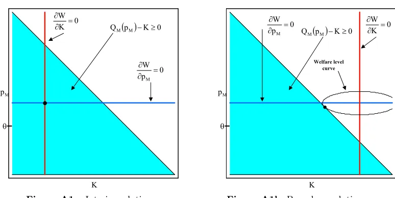
With these functional forms, the first-order condition with respect to price (A.1) is a horizontal line crossing thepM-axis at pM =θ+ [λ/(1 + 2λ)](γ−θ), whereas that with respect to capacity (A.2) is a vertical line crossing theK-axis atK= (θ−c)/ω. See Figures A1a and A1b. The shaded areas correspond to the set defined by the local monopoly output nonnegativity constraint (4) which here is the set of (K, pM) pairs satisfyingK+

pM ≤γ.

0 p W

M

w w

0 K W

w w

K

M

p

T

p K 0

QM M t _p 0

W

M

w w

0 K W

w w

K

M

p

T

Welfare level curve

p K 0 QM M t

Figure A1a:Interior solution Figure A1b:Boundary solution

When (A.3) holds, we obtain the interior solution to (6)-(10) as the intersection of the two lines shown in Figure A1a. More specifically, when

(θ−c)<

_{ω(1 +λ)}

(1 + 2λ) +ω(1 +λ)

(γ−c) (A.6)

the (interior) solution is

K=(θ−c)

ω (A.7)

pM =θ+

λ

1 + 2λ

(γ−θ) (A.8)

This solution corresponds to policy (i) of Proposition 1. When (A.3) does not hold, the boundary solution at the tangency point shown in Figure A1b is obtained. More specifically, when

ω(1 +λ) (1 + 2λ) +ω(1 +λ)

(γ−c)≤(θ−c)<(γ−c) (A.9)

this boundary solution is

K=

1 +λ

(1 + 2λ) +ω(1 +λ)

(γ−c) (A.10)

pM =c+

_{λ+ω(1 +λ)}

(1 + 2λ) +ω(1 +λ)

and corresponds to policy (ii) described in Proposition 1.

Proof of Proposition 1: With (θ−c)< C′_(Q

M), the first-order condition (7) yieldsν= 0 in which case (10) yields 0< K < QM and (6) and (7) are rewritten as (11) and (12). When (θ−c) ≥C′_(Q

M), (7) yieldsν > 0 in which case (10) yields K =QM and (6)

combined with (7) yield (13).

Controlling the regional monopoly with price and transport capacity

Illustration of the program resolution approach: For the purpose of analyzing the solution to (18)-(21) in theK-pM space, we first consider the unconstrained maximization program and then introduce the participation set. An unconstrained welfare maximizer capacity-price pair satisfies the following first-order conditions:

λK+ (pM−θ)Q′M = 0 (A.12)

(1 +λ) [(θ−c)−C′_{(K)] +λ(p}

M−θ) = 0 (A.13)

Second-order conditions for such an unconstrained local social welfare maximizer are syn-thesized by

λQ′

M

λKQ′′

M −Q′M 2 <

(1 +λ)C′′_(K)

λ (A.14)

Observe that, for the welfare function (15),sign[∂2_W/∂K∂p

M(=λ)]>0.30 Hence, under this control scheme without transfers, the social marginal valuation of capacity increases with the regional market price.

In theK-pM space, provided thatQ′′′M ≤0 andC′′′(K)≥0, the first-order condition with respect to price of the unconstrained program (A.12) can be represented by an increasing concave function, with slopeλQ′

M/[λKQ′′M−Q′M 2

], which crosses thepM-axis at pM = θ. Similarly, the first-order condition with respect to capacity (A.13) can be represented by an increasing convex function, with slope (1 +λ)C′′_{(K)/λ, which crosses}

thepM-axis atpM =θ−((1 +λ)(θ−c)/λ)≤θ. These two functions representing (A.12) and (A.13) cross at most twice for anyKand at most once forK >0.

Since (θ−c)>0, atK= 0 the increasing concave function representing (A.12) implies a strictly larger level of price than the one implied by the increasing convex function representing (A.13). Therefore, such functions are expected either to cross only once or not at all. It is straightforward to show that in the case they cross only once, the crossing point, which is a solution to (A.12)-(A.13), satisfies the second-order conditions (A.14) for the unconstrained welfare maximization program.

The participation set is a convex set in the K-pM space when both qm > 0 and

pM > θ. Its boundary has a slopemΠm given by

mΠm =

pM−θ

(QM−K) + (pM−θ)Q′M

= Fm

Q′

MFm+ (QM−K)

2 (A.15)

30_{For a general convex cost function of the regional monopoly, sign[∂}2_W/∂K∂p M] =

sign[λ+C′′

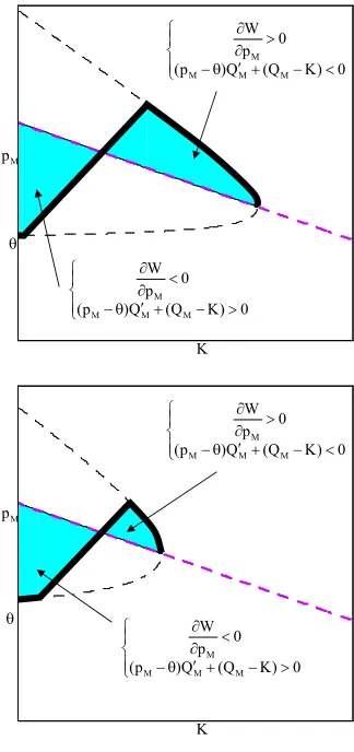
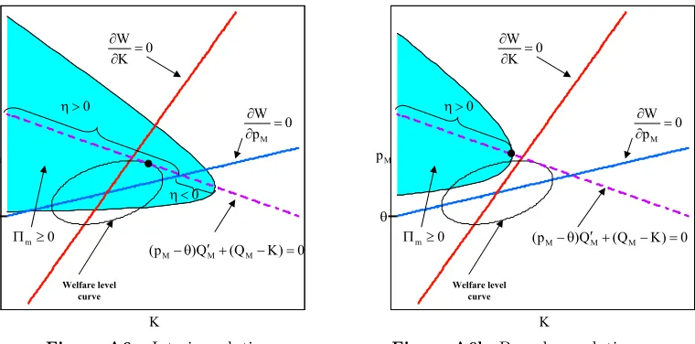
If the capacity-price pair that satisfies (A.12)-(A.14) belongs to the participation set, it will also be a solution to the constrained welfare maximization program. Otherwise, the constrained welfare maximizer is at a tangency point between a welfare level curve and the boundary of the participation set, characterized by:31

mΠm =−

(1 +λ) [(θ−c)−C′_{(K)] +λ(p}

M−θ)

λK+ (pM−θ)Q′_M

(A.16)

Because the shape of the participation set is sensitive to the size of the fixed costFm, closed-form solutions are difficult to obtain. To understand the nature of this difficulty, let us assume for a moment that there is no fixed cost and focus on the region defined by the first-order condition with respect to price (18).

For the functional forms given in (A.5), the function representing the first-order con-dition of the unconstrained program (A.12) is a line of slope λ while that representing (A.13) is a line of slopeω(1 +λ)/λ. From the second-order condition (A.14), the crossing point between these two lines is an unconstrained welfare maximizer if ω(1 +λ)/λ > λ

and this is so independently of the value of the fixed costFm.

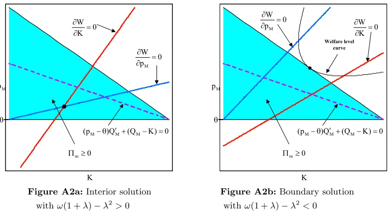
Let us now examine the participation set for the relevant area where pM −θ ≥ 0. WithFm= 0 the boundary of this set will be flat when (pM−θ) = 0 and will have a slope equal to−1 when (pM −θ)>0 and K=QM on this negatively-slopped portion of the boundary. Figures A2a and A2b below show these features. The shaded areas correspond to the participation set defined by (16) and the upward-slopping lines represent the first-order conditions (A.12) and (A.13).

0 p W M w w 0 K W w w 0 ) K Q ( Q ) p

( MT Mc M M p T K 0 mt 3 0 p W M w w 0 K W w w 0 ) K Q ( Q ) p

( MT Mc M Welfare level curve M p T K 0 mt 3

Figure A2a:Interior solution Figure A2b:Boundary solution withω(1 +λ)−λ2_{>0 withω(1 +λ)−λ}2_<0

31_{The second-order conditions for this boundary solution are synthesized by}

(1 +λ)(QM−(1 +λ)K)2C′′(K)Q

′′′

M

−[φ(QM−K) +λK]

(2φ2_{+ 3φ−2λ)(Q}

M−K) +λ(1 + 2λ)K

Q′

M 2

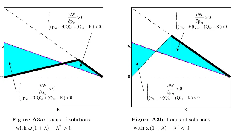
In both of these figures the downward-slopping dashed line represents the (K, pM) pairs satisfying [(pM−θ)Q′M+ (QM−K)] = 0. Figures A3a and A3b below show the geomet-ric characterization of the first-order condition with respect to pgeomet-rice of the unconstrained program (A.12). Provided thatφis nonnegative, the (K, pM) pairs satisfying (18) belong to the shaded areas in these figures. For alternative values of the cost-gapθ−c, we see from (19) that the solution of the constrained program lies on the bold segments shown in Figures A3a and A3b.

M p T °¯ ° ® ­ c T ! w w 0 ) K Q ( Q ) p ( 0 p W M M M M °¯ ° ® ­ ! c T w w 0 ) K Q ( Q ) p ( 0 p W M M M M K K M p T °¯ ° ® ­ c T ! w w 0 ) K Q ( Q ) p ( 0 p W M M M M °¯ ° ® ­ ! c T w w 0 ) K Q ( Q ) p ( 0 p W M M M M

Figure A3a:Locus of solutions Figure A3b:Locus of solutions withω(1 +λ)−λ2_{>0 withω(1 +λ)−λ}2_<0

Now, when we proceed to generalize this argument to the case where Fm > 0, the bold segments representing the solution to the constrained program in Figures A3a and A3b become curves, and more importantly, their shapes are sensitive to the size of the fixed cost. Figures A4a and A4b below show these bold curves for two different values of

Fmwith those on the upper parts corresponding to a lower fixed cost than those on the lower parts. Cross-examining Figures A2a-A2b and A3a-A3b, we see that when there is no fixed cost solutions with φ >0 happen only in the negatively-sloped portion of the boundary of the participation set. In contrast, with a positive fixed cost a solution with

M p T °¯ ° ® ­ c T ! w w 0 ) K Q ( Q ) p ( 0 p W M M M M °¯ ° ® ­ ! c T w w 0 ) K Q ( Q ) p ( 0 p W M M M M K M p T °¯ ° ® ­ c T ! w w 0 ) K Q ( Q ) p ( 0 p W M M M M °¯ ° ® ­ ! c T w w 0 ) K Q ( Q ) p ( 0 p W M M M M K M p T °¯ ° ® ­ ! c T w w 0 ) K Q ( Q ) p ( 0 p W M M M M K M p T °¯ ° ® ­ c T ! w w 0 ) K Q ( Q ) p ( 0 p W M M M M °¯ ° ® ­ ! c T w w 0 ) K Q ( Q ) p ( 0 p W M M M M K

Figure A4a:Locus of solutions Figure A4b:Locus of solutions withω(1 +λ)−λ2_>0,F

m>0 withω(1 +λ)−λ2 <0,Fm>0

Proof of Proposition 2: Sinceθ−c >0, the functions representing (A.12) and (A.13) do not cross atK = 0, but we know that they cross at most once at a point whereK >0. However, a policy that prescribesK = 0 might still be optimal ifFm is high enough to satisfy (22) with equality. These features characterize policy (i) given in the proposition.

If a crossing point of the functions representing (A.12) and (A.13) exists and belongs to the participation set (in which caseqm>0), i.e., using (21) and (A.12), ifFm<−λK(QM_Q′−K)

M , this interior point, which from (A.13) is characterized by (1 +λ)[c+C′_(K)]

−λpM =θ, is picked up as the solution of the constrained welfare maximization program. Such crossing point is defined byλ2_{K= (1+λ)Q}′

M[(θ−c)−C′(K)], rewritten as (26), which results from (A.12) and (A.13), rewritten as (24) and (25). Now, to guarantee that it exists, solving (26) forλ2 and substituting into the second-order conditions (A.14) yields the technical conditionQ′

M

h C′′_(K)

−C′K(K)

i − λK

Q′

MQ

′′

MC′′(K)<0. This characterizes policy (ii-a).

lies outside the participation set, the optimization program picks the boundary solution satisfying (18), (19), and (A.16). These conditions are rewritten, respectively, as (27),

(28) and (29). This corresponds to policy (ii-b).

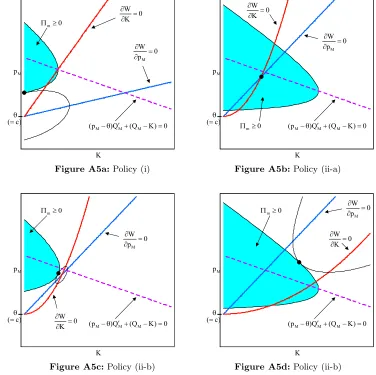
Figures A5a-A5d illustrate these policies for specific functional forms in theK−pM space for the simplified case under which the cost gap (θ−c) converges to cero.32

0 p W M w w 0 K W w w 0 ) K Q ( Q ) p

( MT cM M M p T K 0 mt 3 ) c ( 0 p W M w w 0 K W w w 0 ) K Q ( Q ) p

( MT Mc M M p T K 0 mt 3 ) c (

Figure A5a:Policy (i) Figure A5b:Policy (ii-a)

0 p W M w w 0 K W w w 0 ) K Q ( Q ) p

( MT cM M M p T K 0 mt 3 ) c ( 0 p W M w w 0 K W w w 0 ) K Q ( Q ) p

( MT Mc M M p T K 0 mt 3 ) c (

Figure A5c:Policy (ii-b) Figure A5d:Policy (ii-b)

32_{Figure A5a is based on the functional forms (A.5), (λ, ω, γ, θ = c)}

∈ {(1/3,1/2,10,2),(3/2,1/2,10,2)}, respectively, and Fm = 10.24. Figures A5b and A5c employ the linear demand in (A.5), the capacity building cost function C(K) = (ω

3K+ σ 2)K

2_{, (λ, ω, σ, γ, θ= c) ∈ {(3/2,1/2,1/200,10,2),(3/2,1/15,1/200,10,2)}, and}

Controlling the regional monopoly with transport capacity only

Illustration of the program resolution approach: Turning to the study of the solution to the system (33)-(37) in theK-pM space, observe that since social welfare under this control scheme is the same as that in the previous section, so is the analysis of the unconstrained maximization program. When constraints are introduced in the maximization program, however, an additional one arises here, namely, the profit-maximization constraint (31). Such a constraint is represented in theK-pM space by a decreasing concave function with slope −Q′

M/[(QM −K)Q′′M −2Q′M 2

] and intercept point strictly in the interior of the participation set. Furthermore, this function crosses the boundary of the participation set at a point where the latter is infinitely sloped.33

Equation (33), (34), and (37) define a tangency point between a welfare level curve and the function that represents the profit-maximization constraint. Hence, such a point satisfies

− Q

′

M

(QM−K)Q′′M−2Q′M 2 =

(1 +λ) [(θ−c)−C′_(K)]Q′

M−λ(QM−K) [QM −(1 +λ)K]Q′M

(A.17)

If such a tangency point satisfies the firm’s participation constraint (36) with a strict inequality, it is an interior solution.34 Note from (A.17) thatK = 0 cannot be a tan-gency point, and hence not an interior solution. If such a tantan-gency point violates (36), the solution to (33)-(37) lies at the intersection of the function representing the profit-maximization constraint and the boundary of the participation set where, recall, the latter is infinitely sloped.35

Let us illustrate the solution under this control scheme using the functional forms (A.5). In this case, the set defined by the firm’s profit maximization constraint (31) is a line of slope−1/2 that crosses the boundary of the participation set at the point where the latter is infinitely sloped, as shown in Figures A6a and A6b. The shaded regions correspond to the participation set defined by (30). The upward-slopping lines represent the price and capacity first-order conditions of the unconstrained program, respectively, (A.12) and (A.13). The downward-slopping dashed line is the set of (K, pM) pairs which satisfy the profit-maximization constraint of the local monopoly (31).

33_{The reader can check that such a crossing point is characterized by the condition}

Fm (QM(pM)−K)

=−(QM(p_QM′)−K)

M

Solving forFm and substituting into the expression of the slope of the boundary of the participation set (A.15) yields the slope of this set at the crossing point.

34_{Second-order conditions are synthesized as:}

−Ω2(1 +λ)C′′_{(K) + 2λΩ}

−

(QM−K)(Q′′M −ηQ′′′M)

Q′

M

+ [Q′

M−3ηQ′′M]<0

Note that for a downward-sloping linear demand, the former condition holds for any value ofη.

35_{In this case, second-order conditions are always satisfied. It is worthwhile noting that}

0 p W M w w 0 K W w w 0 ) K Q ( Q ) p

( MT cM M

Welfare level curve 0 ! K 0 K M p T K 0 mt 3 0 p W M w w 0 K W w w 0 ) K Q ( Q ) p

( MT Mc M

Welfare level curve 0 ! K M p T 0 mt 3 K

Figure A6a:Interior solution Figure A6b:Boundary solution

Figure A6a sketches the case in which the solution lies in the interior of the partici-pation set. This interior solution is

K=(1 + 2λ)(γ−c) + (3 + 2λ)(θ−c)

1 + 4λ+ 4ω(1 +λ) (A.18)

pM =θ+[λ+ 2ω(1 +λ)] (γ−c)−(θ−c) [2 + 3λ+ 2ω(1 +λ)]

1 + 4λ+ 4ω(1 +λ) , (A.19)

and emerges when the condition

(θ−c)< (γ−c) [λ+ 2ω(1 +λ)]− √

Fm[1 + 4λ+ 4ω(1 +λ)]

2 + 3λ+ 2ω(1 +λ) (A.20)

holds. It represents policies of type (i) in the proposition. When condition (A.20) does not hold, the solution is on the boundary of the participation set. Figure A6b shows such a boundary solution given by

K=γ−θ−2√Fm (A.21)

pM =θ+

√

Fm (A.22)

This solution represents the policies of type (ii) in Proposition 3.

Proof of Proposition 3: Before sketching the proof, let us recall from our discussion that precedes the proposition in the text thatK = 0 is never a solution to the constrained welfare maximization program.

Since (θ−c)>0 and Fm>0, the capacity-price pair that maximizes the firm’s profit, defined by (37), belongs to the participation set if (36) holds with a strict inequality, i.e., if the fixed cost belongs to the intervalFm<−(Qm−K)

2

Q′

M . Since by definition an interior solution satisfies (A.17), which stems from (33), (34), and (37), pricing and capacity building obey (38)-(40). Finally, given thatφ= 0, (34) can be rewritten as (1 +λ)[c+

C′_(K)]