ELISA validation in the pharmaceutical industry: a mixed effects models approach with R

Texto completo

(1)

(2)

(3)

(4)

(5)

(6) Contents List of Figures. 3. 1 Project information. 5. 1.1. Context and rationale . . . . . . . . . . . . . . . . . . . . . . . . . . . . . . . . . . .. 5. 1.2. Objectives . . . . . . . . . . . . . . . . . . . . . . . . . . . . . . . . . . . . . . . . . .. 6. 1.2.1. Global objectives . . . . . . . . . . . . . . . . . . . . . . . . . . . . . . . . . .. 6. 1.2.2. Specific objectives . . . . . . . . . . . . . . . . . . . . . . . . . . . . . . . . .. 6. 1.3. Applied methodology . . . . . . . . . . . . . . . . . . . . . . . . . . . . . . . . . . . .. 6. 1.4. Project planning . . . . . . . . . . . . . . . . . . . . . . . . . . . . . . . . . . . . . .. 7. 1.5. Summary of results . . . . . . . . . . . . . . . . . . . . . . . . . . . . . . . . . . . . .. 8. 1.6. Summary of chapters . . . . . . . . . . . . . . . . . . . . . . . . . . . . . . . . . . . .. 8. 2 Introduction. 10. 2.1. Principles of ELISA assays. 2.2. Bioassay validation . . . . . . . . . . . . . . . . . . . . . . . . . . . . . . . . . . . . . 12. 2.3. . . . . . . . . . . . . . . . . . . . . . . . . . . . . . . . . 10. 2.2.1. Accuracy . . . . . . . . . . . . . . . . . . . . . . . . . . . . . . . . . . . . . . 12. 2.2.2. Precision . . . . . . . . . . . . . . . . . . . . . . . . . . . . . . . . . . . . . . 12. 2.2.3. Parallelism . . . . . . . . . . . . . . . . . . . . . . . . . . . . . . . . . . . . . 14. Mixed effects models . . . . . . . . . . . . . . . . . . . . . . . . . . . . . . . . . . . . 15 2.3.1. Rationale behind mixed models . . . . . . . . . . . . . . . . . . . . . . . . . . 15. 2.3.2. Fixed and random effects . . . . . . . . . . . . . . . . . . . . . . . . . . . . . 16. 2.3.3. Nested and crossed effects . . . . . . . . . . . . . . . . . . . . . . . . . . . . . 16. 2.3.4. Statistical model formulation . . . . . . . . . . . . . . . . . . . . . . . . . . . 17. 2.3.5. Parameter estimation . . . . . . . . . . . . . . . . . . . . . . . . . . . . . . . 22. 2.3.6. Evaluating significance . . . . . . . . . . . . . . . . . . . . . . . . . . . . . . . 24 1.

(7) 2. CONTENTS. 3 Part I: Analysis of validation studies 3.1. 3.2. 3.3. Validation study 1 . . . . . . . . . . . . . . . . . . . . . . . . . . . . . . . . . . . . . 28 3.1.1. Data structure . . . . . . . . . . . . . . . . . . . . . . . . . . . . . . . . . . . 28. 3.1.2. Analysis . . . . . . . . . . . . . . . . . . . . . . . . . . . . . . . . . . . . . . . 30. 3.1.3. Inference . . . . . . . . . . . . . . . . . . . . . . . . . . . . . . . . . . . . . . 36. 3.1.4. Validation . . . . . . . . . . . . . . . . . . . . . . . . . . . . . . . . . . . . . . 41. Validation study 2 . . . . . . . . . . . . . . . . . . . . . . . . . . . . . . . . . . . . . 45 3.2.1. Data structure . . . . . . . . . . . . . . . . . . . . . . . . . . . . . . . . . . . 45. 3.2.2. Analysis . . . . . . . . . . . . . . . . . . . . . . . . . . . . . . . . . . . . . . . 48. 3.2.3. Inference . . . . . . . . . . . . . . . . . . . . . . . . . . . . . . . . . . . . . . 52. 3.2.4. Validation . . . . . . . . . . . . . . . . . . . . . . . . . . . . . . . . . . . . . . 55. Comments on study designs . . . . . . . . . . . . . . . . . . . . . . . . . . . . . . . . 58. 4 Part II: Analysis of parallelism studies 4.1. 28. 59. Parallelism study 1 . . . . . . . . . . . . . . . . . . . . . . . . . . . . . . . . . . . . . 59 4.1.1. Data structure . . . . . . . . . . . . . . . . . . . . . . . . . . . . . . . . . . . 59. 4.1.2. Analysis . . . . . . . . . . . . . . . . . . . . . . . . . . . . . . . . . . . . . . . 61. 4.1.3. Model check and refit . . . . . . . . . . . . . . . . . . . . . . . . . . . . . . . 66. 4.1.4. Parallelism validation . . . . . . . . . . . . . . . . . . . . . . . . . . . . . . . 70. 5 Conclusions. 72. 6 Glossary. 74. 7 R code appendix. 75. 7.1. 7.2. Custom functions for the lme4 package . . . . . . . . . . . . . . . . . . . . . . . . . . 75 7.1.1. tablefixef function . . . . . . . . . . . . . . . . . . . . . . . . . . . . . . . . . 75. 7.1.2. tablevarcomp function . . . . . . . . . . . . . . . . . . . . . . . . . . . . . . . 75. 7.1.3. tableanova function . . . . . . . . . . . . . . . . . . . . . . . . . . . . . . . . . 76. 7.1.4. tableconfint function . . . . . . . . . . . . . . . . . . . . . . . . . . . . . . . . 76. 7.1.5. diagplots function . . . . . . . . . . . . . . . . . . . . . . . . . . . . . . . . . . 76. Custom functions for the nlme package . . . . . . . . . . . . . . . . . . . . . . . . . . 77 7.2.1. Bibliography. calcratios function . . . . . . . . . . . . . . . . . . . . . . . . . . . . . . . . . 77 79.

(8) List of Figures 1.1. Gantt diagram for temporal planning including task names. . . . . . . . . . . . . . .. 7. 2.1. Execution phases for a sandwhich type ELISA. . . . . . . . . . . . . . . . . . . . . . 11. 2.2. Example of a 4 parameter logistic function fitted to real data. The function defining parameters are shown identified by the greek letter ϕ plus a subindex. . . . . . . . . 21. 3.1. Boxplot of raw data by grouping factor analyst (A) or day (B). . . . . . . . . . . . . 29. 3.2. Levelplots displaying the number of observations at each variable combination. . . . 30. 3.3. Diagnostic plots for data11.mod1 model. . . . . . . . . . . . . . . . . . . . . . . . . . 34. 3.4. Response values (rp) for M3 samples with observation 51 in red. . . . . . . . . . . . 35. 3.5. Diagnostic plots for data11.mod2 model adjusted without observation 51. . . . . . . 37. 3.6. Relative bias plot for validation study 1. . . . . . . . . . . . . . . . . . . . . . . . . . 42. 3.7. Computational cost for the % CV bootstrap CI calculation. . . . . . . . . . . . . . . 45. 3.8. Boxplot of raw data by grouping factor analyst (A), day (B) or laboratory (C). . . . 46. 3.9. Levelplots displaying the number of observations at each variable combination. . . . 47. 3.10 Diagnostic plots for data12.mod1 model. . . . . . . . . . . . . . . . . . . . . . . . . . 49 3.11 Diagnostic plots for data12.mod2 model. . . . . . . . . . . . . . . . . . . . . . . . . . 51 3.12 Diagnostic plots for data12.mod4 model. . . . . . . . . . . . . . . . . . . . . . . . . . 53 3.13 Relative bias plot for validation study 2. . . . . . . . . . . . . . . . . . . . . . . . . . 56 4.1. Scatter plots of raw data by grouping factor day (A) or plate (B) colored by serial type and by factor serial type colored by plate (C). . . . . . . . . . . . . . . . . . . . 60. 4.2. Diagnostic plots for the residuals of data21.mod1 object. A) residuals vs. fitted values, B) QQplot against a normal distribution. . . . . . . . . . . . . . . . . . . . . 66. 4.3. Plot of data21.mod1 model residuals against the logarithm of the dilution. . . . . . . 67. 4.4. Comparison of the residuals against log-dilution plots from the data21.mod3 variance corrected model (A) and data21.mod1 non-corrected model (B). . . . . . . . . . . . 69. 4.5. QQplots to check the random effects structure for each model parameter for the data21.mod3 model. . . . . . . . . . . . . . . . . . . . . . . . . . . . . . . . . . . . . 70 3.

(9) 4. LIST OF FIGURES 4.6. Asymptote and scale parameters ratios 90 % confidence intervals and the 0.9-1.1 acceptability region. . . . . . . . . . . . . . . . . . . . . . . . . . . . . . . . . . . . . 71.

(10) Chapter 1. Project information 1.1. Context and rationale. This project has been developed within the bioassay validation frame, specifically concerning the Enzyme-Linked Immunosorbent Assays (ELISA) [2] in the context of veterinary pharmaceutical industry. Consequently, methodology applied has been subject to the requirements of two of the most influential regulatory agencies: the United States Department of Agriculture (USDA) and the European Medicines Agency (EMA)[53, 16]. To adapt the complexity of this endeavour to the available time, the degree of fulfilment of these guidelines has been lowered and only the most critical aspects have been considered. The project and subsequent report have been organized in two parts both concerning to different aspects of the validation process of an ELISA assay but nevertheless they are closely related. The first part is centered around the analysis of validation designs intended to quantify the accuracy and precision of the assays. In this kind of assays, one to several distinct product preparations are tested at different locations, at different time points and by different laboratory technicians. Accordingly, resulting data has a longitudinal component but also other grouping structures given by the different factors considered. Due to this complex design structure the application of linear mixed effects models [44] has been tested as an alternative to classical statistical procedures with the final objective to comply with the recommended workflows and information required by the authorities [61]. The second part is devoted to the use of non-linear mixed effects models [44] to analyse ELISA data obtained from full dose-response experiments. In these experiments, the objective is to establish what is known as relative potency (RP) of the test preparation with respect to a pre-specified reference product of known properties. To calculate the RP, an appropriate model for the observed dose-response relationship needs to be specified. In this work, the 3-parameter logistic model has been used to describe this data generating process with the objective to obtain estimates of the defining curve parameters from whom to establish an RP. Previously though, parallelism between the test and reference serials dose-response curves should be demonstrated. The core of this part of the work has been to establish an appropriate workflow to attain this objective following the available regulatory documentation [61]. 5.

(11) 6. CHAPTER 1. PROJECT INFORMATION. 1.2. Objectives. Project global objectives express the main statistical objectives of this project. The type of statistical model used in each case has served as a basis to further divide the work in two different and independent parts. Each part has then its specific objectives which relate to particular tasks that have been executed.. 1.2.1. Global objectives. • Part I: Analyse and interpret two ELISA validation studies using linear mixed effects models. • Part II: Analyse and interpret ELISA dose-response data obtained from a single experiment using 3-parameter logistic non-linear mixed effects models.. 1.2.2. Specific objectives. 1. Part I: 1.1 Correctly determine the data structure (nesting, crossing…). 1.2 Application of linear mixed effects models to analyse the chosen data. 1.3 Offer a correct interpretation of the results in the validation context. 1.4 Generate an R markdown script to automatically analyse and report from the chosen study designs. 1.5 Identify weak points in the analysed designs and propose how to improve them. 2. Part II: 2.1 Analysis of ELISA dose-response curves using non-liner mixed effect models. 2.2 Interpret and make inference on the model parameters. 2.3 Calculate the asymptote and scale parameter ratios between a reference and a test serial based on a NLME model parameter estimates. Write an R script to automate this task. 2.4 Calculate confidence intervals for the previously mentioned ratios using the delta method. Write an R script to automate this task.. 1.3. Applied methodology. Three possible methodologies were identified at the beginning of the project, namely: 1. Start with a learning phase used to search and understand the theory of mixed effects models followed by a phase for experimenting with the available software packages and finally a phase where this previous knowledge is used on real data. 2. Start by applying the procedures described in software documentation to analyse sample data directly to real data and gain knowledge in a parallel way. 3. Start with a learning phase for the theory of mixed models based on a practical approach using sample data. Finally, apply the gained knowledge to the analysis of real data..

(12) 1.4. PROJECT PLANNING. 7. Figure 1.1: Gantt diagram for temporal planning including task names.. Initially strategies 1 and 3 were considered appropriate as both considered a learning period. Strategy 1 is a more classical approximation with practical learning following the theoretical one whereas strategy 3 is a learning-by-doing kind of strategy where theory and practice are considered in parallel. Strategy 2 was considered too risky from the beginning considering the theoretical challenge that mixed effects models represent. Following careful analysis and considering the director of the work recommendation, strategy 1 has been applied. It was considered that enough time was available to make this classical yet more robust approach.. 1.4. Project planning. No special resources have been needed or employed to develop this project. Availability of real data to analyse during the course of the project has been granted thanks to the collaboration of Laboratorios Hipra S.A., affiliation of the author at the time of execution of this work. Initial task planning has been subject to minor modifications in light of several events occurred during the execution, none of them critical. Justification and detailed explanation was given in the intermediate reports presented during the project development. The actual executed temporal planification and the several tasks that have conformed the project are presented in form of a Gantt diagram (Figure 1.1)..

(13) 8. CHAPTER 1. PROJECT INFORMATION. 1.5. Summary of results. Results of this project include: • This thesis, which includes an extensive bibliography review about mixed-effects models and demonstrates their implementation in distinct situations relevant to pharmaceutical validation. • The R markdown document obtained as result of Part I containing common R syntax and custom functions to properly analyse validation studies using linear mixed effects models. • The R script obtained as a result of Part II containing a custom function to calculate ratios and confidence regions for model parameters of a 3-parameter logistic non-linear mixed effects model. This is not included as a separate file but instead it can be found in Section 7.2.1. • Intermediate progress reports obtained as a result of PAC 2 and PAC 3 containing relevant project follow-ups and updates. • The final presentation that will be delivered according to the planned schedule.. 1.6. Summary of chapters. As mentioned above, the work in this project has been organized in two parts each of them centered around an important topic in bioassay validation. Chapter 1 contains relevant information about the project itself as the rationale behind it and the list of global and concrete objectives that have been accomplished. Also, the real executed task planification is reported accompanied with the final list of products obtained. Chapter 2 is an introductory text built through an in-depth bibliography review. Starting from the basic concepts related with ELISA bioassays the text guides the reader through the most important regulatory recommendations and obligations and ends with an extensive text covering the basic concepts related with mixed models. As an statistical centered project, this last part is extensive and covers the rationale behind the need for mixed models and its mathematical formulae. Also several important concepts are explained such as the meaning of random effects or nesting structures in designs. Most importantly, the end of the chapter covers the issue of testing the statistical significance of the model parameters which is an area of active research far from being closed or well established. Chapter 3 covers the analysis of two ELISA validation studies each of them with some particularities, such as different number of random effects or model structure. Appropriate model fitting of linear mixed effects models with the R lme4 package and model diagnostics is explained followed by a section on how to practically test statistical significance of both fixed and random effects, knowing that this is not a closed issue. Finally, a validation section covers the main objective of the analysis: check the performance of the assay based on accuracy and precision criteria. Chapter 4 covers the fitting of a 3-parameter logistic mixed effects model for ELISA raw doseresponse curves accounting for the grouping structure. Model fitting with the nlme R package is covered alongside the basic model diagnostics and inference on the parameters. Once the model is.

(14) 1.6. SUMMARY OF CHAPTERS. 9. obtained, parameter estimates for both a test and a reference serial preparations are used to demonstrate how to calculate the asymptote and scale factor ratios and their accompanying confidence intervals to check if curve parallelism can be assumed. Chapter 5 contain the final thoughts regarding the lessons learned from the project, the degree of fulfilment of the initial objectives and a critical comment with respect the task planning and project execution. Also, some comments on future issues to explore are detailed there. Chapter 7 contain all custom R code used during this work. All functions are properly annotated explaining possible dependencies, requirements and intended use..

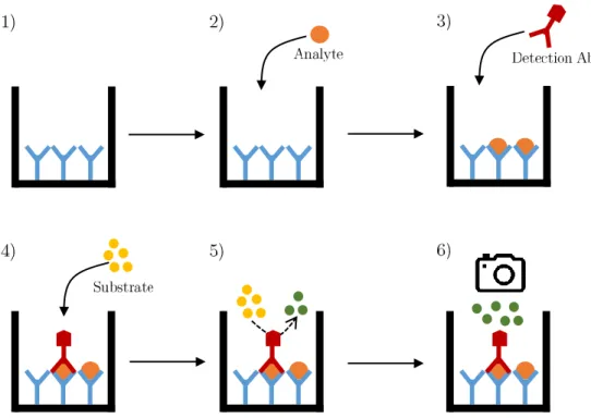
(15) Chapter 2. Introduction 2.1. Principles of ELISA assays. Biologically-based analytical methods to quantify specimens (bioassays) are the group of techniques that rely on the use of biological reagents, such as antibodies, live cells, etc., to quantify a substance of interest. This substance of interest is usually called analyte and, in the pharmaceutical vaccine industry, the analyte is in turn usually an antigen. The antigen is the substance that, when appropriately formulated, triggers an immune response from the immune system of a given animal [59]. The term antigen is a wrapper as the chemical structure of antigens is diverse ranging from purified proteins to lipids or, for example, whole cells of a given bacterium [59]. As diverse as the nature of the antigen is the type of immune response. Two basic types are antibody-based or cellmediated and which type is generated greatly depends on the type of antigen and its accompanying adjuvants, which substances that are used to stimulate or boost the immune response. Also, immune responses are complex in that they are usually not exclusively of one type or another [23]. Enzyme-Linked Immunosorbent Assays or ELISA(s) are a type of bioassay in that they are based on the antigen-antibody recognition. Antibodies are generated such as they are specific against a given antigen or family of antigens. Thus, as the antigen-antibody interaction is specific, this property can be used to selectively find a molecule in a mixture of constituents, such as a vaccine. ELISAs make use of this property to specifically quantify analytes of interest in complex solutions, even in very low quantities [2]. Several types of ELISA exist that are used preferentially for different purposes as their properties, also varying, makes each type best suited for a particular task [2]. In the pharmaceutical industry, all types are used to quantify antigens in vaccines as the type performance is difficult to predict and selection is usually product dependent made by trial and error. Despite this, here the sandwich type will be explained as it is favoured by some authorities [52] and it is also widely implemented due to its outstanding sensivity [2]. This type is based in the use of two antibodies which are added in a sequential order and trap the antigen in between them to achieve a selective recognition. The second antibody is pre-labelled with a marker which is able to produce some sort of detectable signal (colour, light or fluorescence) by itself or when a substrate is added [2]. To gain a better understanding of the explained protocol, Figure 2.1 depicts the fundamental method to execute a sandwich ELISA. First, a solid support is coated with the capture antibody (1). After that, the product which contains the analyte to be detected is added (2). This causes the 10.

(16) 2.1. PRINCIPLES OF ELISA ASSAYS. 11. Figure 2.1: Execution phases for a sandwhich type ELISA.. formation of antigen-antibody complexes throughout the coated surface but, as capture antibody is used in excess, it is expected that some binding sites remain empty. Then, the detection antibody is added (3). Before that, this antibody has been chemically bounded to an enzyme which is able to produce a detectable signal by some type of chemical method. Usually, these enzymes chemically decompose a colourless substrate into a coloured product. Once the detection antibody-antigen complexes have formed, the sandwhich is obtained. Finally, the substrate is added (4), allowed to react during a specified amount of time (5) and the resulting signal is then measured (6) using an imager or some other detector. It should be noted that the arrows between phases indicate in-between procedures that are omitted for clarity. These procedures are incubations, usually conducted at a given temperature for a given period of time, and washes, that are used to remove unused products at the end of a step before proceeding to the next. As the solid support used is usually a microtiter plate of at least 96 wells, the black “U” shaped solid lines represent each one of this wells.. The final result of a usual assay are signal lectures for each well in a plate. The intensity of the signal of a well is proportional to the amount of analyte present during the assay, thus, by combining this procedure with dilution techniques, analysts are able to produce saturation to extinction response curves depending on the concentration of the analyte which finally can be used to quantify it. A close example of a quantification procedure albeit for other purposes, will be explained in Section 4..

(17) 12. 2.2. CHAPTER 2. INTRODUCTION. Bioassay validation. ELISAs are a crucial tool in the manufacturing and quality control of pharmaceutical products. The production of pharmaceutical products is strictly regulated under the auspices of the Good Manufacturing Practices, or GMP, which demand all quantification methods used to characterize a product to meet certain standardized accuracy and precision criteria [61]. Validation is the process of demonstrating and documenting that a certain type of assay, which has been designed for a particular purpose (e.g. determine an analyte concentration), it is in fact suitable for the task and results in accurate and reliable results which can be appropriately reproduced [61, 16]. Validation process is extensive [20] and it is intended to characterize every aspect of a certain quantification method. Regulatory agencies, sometimes through child agencies or through pharmacopeial compendiums, issue their own guidelines on how to conduct the tests and report the results ensuring, at least, that common standards are meet inside their influence zones. These guidelines include a mixture of recommendation and unavoidable requirements and constitute the regulatory framework to which the pharmaceutical industry is bounded [61, 16]. At least 10 parameters need to be evaluated to complete a full validation protocol [1] but in this work only accuracy, precision and parallelism will be considered.. 2.2.1. Accuracy. Accuracy is defined as the closeness of the value obtained by a certain method to the real value or a theoretically expected value so, it is a performance measure that quantifies any systematic bias the assay might have. In this work, formulation provided by the United States Pharmacopoeia (USP) [62], which is usually more restrictive than the European Pharmacopoeia (Ph.Eur.), is used. Thus, accuracy is to be reported in the form of a relative bias using percent units, % RB, using the following expression: (. Actual value RB(%) = 100 −1 Expected value. ). (2.1). Usually the RB value is reported alongside a confidence interval. As the actual value used in the calculations is a parameter estimate of a mixed-effects model and the expected value is the theoretical value used to prepare the product and is a known constant, upper and lower confidence interval limits for the actual value, which are easily extracted from the model summary, can be used to calculate approximate confidence intervals by using the same formula.. 2.2.2. Precision. Precision is defined as the closeness of repeated individual measures of the analyte and thus it is a performance value that relates to random variation introduced by potential nuisance factors. Is a more complex term than accuracy and it is usually evaluated at three distinct levels: repeatability, reproducibility and intermediate factor precision [45]. Repeatability is the variability observed when the assay is independently conducted several times under the same conditions within a short period of time. By the “same” conditions it must be understood to held as many factors as possible at a constant value. On the contrary, reproducibility is the variability observed when the assay is independently replicated several times but under.

(18) 2.2. BIOASSAY VALIDATION. 13. changing conditions and over a longer period of time. In this case, the assay protocol is maintained but the rest of factors potentially affecting its performance, e.g. laboratory and analyst, are allowed to change. Finally, intermediate factor precision is the variability observed when all factors except one are allowed to change. For example, intermediate laboratory precision would be measured by repeating the assay several times in the same laboratory under normal operating conditions but by different analysts and using different lot reagents [1, 62, 45]. Estimation of precision values is difficult [1] but the use of mixed-effects models makes it easier as variance components for a given model are a natural outcome of the analysis. In this way, estimates of the three types of precision measures considered can be obtained by combining the different variance component estimates [1, 65]: • Repeatability (r) is estimated by the residual model variance: σr2 . • Intermediate factor precision (ifp) is estimated from the sum of the residual variance and the variance component estimate for the factor of interest: σr2 + σf2actor . Obviously the factor of interest should have been considered in the model specification. • Reproducibility (R) is estimated as the overall variance taking into account all variance component estimates derived from the model: σr2 + σf2actor1 + σf2actor2 + ... + σf2actorn . Usually, variance components are reported in the form of a percent coefficient of variation (CV) which is basically a way to standardize precision estimates to make them comparable between assays [1, 16]. A CV is a formally a ratio between a variance estimate and a related expected value, e.g. the CV for repeatability when a single sample is tested in the assay would be the residual variance estimated by the model divided by the mean quantification value of the sample in question. If percent transformed, then the % CV is obtained. Formulation to obtain the CV is: . CV (%) = 100 . √. . σi2. E(analyte). . (2.2). where i indexes the type of precision CV to be obtained so, as stated above, i = r, ifp or R and thus √ 2 2 the computation of σi changes accordingly. Note that the expression σi is used to calculate the variance in standard deviation units thus, if variance components are readily available in standard deviation units, this expression can be directly substituted by σi . E(analyte) represents an estimate of the expected value for the analyte used in the assay and it will usually be, for example, the mean concentration value for a given product preparation. However, it is not always the case that reporting a CV is appropriate. When data is log-transformed and response is assumed to follow log-normal distribution the percent geometric standard deviation (% GSD) is recommended by the USP [62]. In this case formulation to obtain the % GSD is: √ GSD(%) = 100(exp. σi2. − 1). (2.3). where σi2 has the same interpretation as before. Other formulations are proposed that are demonstrated to work better in certain circumstances [65] but, as the above formulation is explicitly stated in the official guidelines, its use is recommended..

(19) 14. CHAPTER 2. INTRODUCTION. Finally, the above presented point estimates for either CV or GSD are usually reported with a confidence interval. Confidence intervals for ratios are difficult to calculate and, although several approximations exist [25], here they are calculated using bootstrap as it will be demonstrated in Section 3.. 2.2.3. Parallelism. Quantification of an analyte using an ELISA is usually based on establishing a relative potency (RP) of a test product with respect to previously characterized reference product. Thus, RP is simply a ratio of the estimated potency of the test and reference products and it takes the following form [18, 60]:. RP =. P otency(test) P otency(ref erence). (2.4). The terms labelled Potency can be estimated by several means but, in this work, they will be estimated as the location parameters of a logistic model equation fitted to full dose-response data. This is extensively explained in Sections 2.3.4.2.1 and 4. A key aspect for the potency of an unknown product to be established in this way is to ensure that dose-response curves between products are “equivalent”. This requirement, present in all regulatory documents [61, 62, 63, 16, 53], is known as parallelism and is an unavoidable requisite to compute valid RP estimates. Conformance to this requirement is demonstrated by reporting the ratios between the same model parameters individually estimated for both the reference and the unknown products. If this ratios are not found to be significantly different from 1, then parallelism is granted and RP estimates are considered valid. On the contrary, if these ratios fall outside a predefined acceptability zone, parallelism can not be assumed and no RP estimate should be calculated [53, 63]. For a 3-parameter logistic model (3PL) these parameters are the upper asymptote and scale factor (see Section 2.3.4.2.1). As usual, point estimates of validation parameters are to be reported alongside a confidence interval. The confidence interval can be then used to establish if the parameter is likely to fall within the acceptability region. However, to calculate confidence intervals for ratios is not easy. For example, as ratios are the quotient of two quantities, a problem arise if the denominator value is close to zero as it leads to an undefined situation. Moreover, this in turn causes distributional complexities and, for example, neither an expected value nor a variance are defined for a ratio [25, 42, 54]. Due to these issues, among others, confidence intervals for ratios are calculated through several approximations. Two methods will be employed here: the Fieller and delta methods. Whereas the Fieller method is considered to be the standard solution by the USP [63], the delta method, based on a Taylor expansion series, it is far simpler if appropriate assumptions are met. Those assumptions are: 1) denominator significantly different from zero and 2) denominator low standard error. Formulas shown below are based on the article by Franz, H.V. (2007) [25]. The USP provides a different formulation for the Fieller confidence intervals that otherwise is equivalent to the one described here [63]. For the delta method, mathematical expression of the ratio and its confidence region is:.

(20) 2.3. MIXED EFFECTS MODELS. 15 √. CIupper/lower = ρ̂ ± tq |ρ̂|. σ̂x2 σ̂y2 σ̂xy + 2 −2 x̂2 ŷ x̂ŷ. (2.5). where ρ̂ = ŷ/x̂ is the ratio and ŷ and x̂ are (unbiassed) estimators for the quantities of interest, in this case, the location parameters for the test and reference serials respectively. σ̂x2 and σ̂y2 are the estimators for the variance and σ̂xy is the estimated covariance between x̂ and ŷ. Term tq represents the (1 − α/2) quantile of a t-distribution with degrees of freedom equal to the number of plates minus 3 according to CVB-USDA [51]. For the Fieller method formulation is expressed as:. CIupper/lower =. (x̂ŷ − t2q σ̂xy ) ±. √. (x̂ŷ − t2q σ̂xy )2 − (x̂2 − t2q σ̂x2 )(ŷ 2 − t2q σ̂y2 ) x̂2 − t2q σ̂x2. (2.6). where the all the terms have the same interpretation as in Equation (2.5). It should be noticed that both formulations are only valid if the denominator term of the ratio is significantly different from zero at the same significance level used to calculate the term tq . Other limitations exist but they are out of the scope of this work so the reader is referred to the original reference for a complete discussion [25].. 2.3 2.3.1. Mixed effects models Rationale behind mixed models. The standard general linear model, also called ordinary least squares (OLS) regression, allows to describe the relationship between one or more predictor variables (categorical or continuous) and a response in a linear way. The modelled relationship however depends on the fulfilment of several assumptions made during the statistical derivation of the regression method. One of the most critical assumptions is that model residuals (error estimates) are independent and identically distributed (henceforth iid) with an expected value of zero and constant variance. This can be mathematically expressed as ϵi ∼ iid(0, σ 2 ) [21]. This condition can be separated in two parts. The identically distributed errors implies that samples used to build the model were drawn from the same underlying distribution. Stronger than the former statement is the independent errors assumption. This states that the correlation among residuals is zero or, alternatively, the probability of a residual taking some value is independent of the values the other residuals have [56, 21]. However, in biological fields it is common to have highly structured experimental designs with clustered data or to take several measures on the same experimental unit over time rendering a repeated measures design [30]. In those situations it is expected that residuals (and hence observations) will have some degree of correlation and thus the assumption of independence is not held. For example, in the context of an ELISA assay, if a particular sample is tested at two different laboratories, replicates within each one location are expected to be more similar than replicates between different locations. Violations of the iid assumption leads to an increased type I error rates and standard statistical methods such as ANOVA are not robust against it [56]. A classical method for dealing with correlated observations is the well known repeated measures ANOVA (rmANOVA). This method is technically simple and is based, like the traditional ANOVA,.

(21) 16. CHAPTER 2. INTRODUCTION. in partitioning the variance of the response through sums of squares obtaining the expected mean squares (EMS). Then, by algebraic manipulation variance components can be analytically obtained, at least for the simpler designs [33, 22]. However, this method albeit simple has some major limitations. It requires a perfectly balanced design for the sum of squares decomposition to be unique, otherwise the decomposition method affect the variance estimates. It does not tolerate missing values in the data; usually this situation translates into a complete elimination of the observation. Finally, it is not expandable to complex designs with complex clustering structures often found in biological sciences [22, 33, 32]. In this context, mixed effects models arise as a powerful and flexible methodology that can overcome the limitations of classical methods by accommodating a variety of data structures, balance situations and is also capable of dealing with missing values. These advantages come at a cost of a complex methodology which requires more computational power but the latter should not be an issue nowadays, at least for the vast majority of situations [56, 33].. 2.3.2. Fixed and random effects. In statistical modelling, the response is related to a set of measured predictor variables through several model parameters; one for each variable if they are treated as quantitative or one for each level if they are qualitative (also known as factors). These parameters are values estimated from the data and constitute our most plausible guess on how each variable or variable level relates with the response. These parameters are commonly called effects, but this terminology is more common when they are associated to levels of a factor rather than for continuous predictors [6]. These effects can then be subdivided into fixed or random. In mixed models framework, it is necessary to specify in the model structure if the effect of a particular variable is to be considered fixed, random, or in some cases both. This specification is crucial to correctly interpret model results and make inferences. A model parameter should be considered to be a fixed effect if it is associated to an entire population or to specific and reproducible levels of a factor. Put in another way, if for example the final interest is to make inferences about the specific levels of a factor without any aim to generalize, then this factor should be considered to have a fixed effect. On the other way, if considered as a random effect, the parameter is then a random variable which captures the random variability from known or expected sources of variation (e.g. subject) in the data that would otherwise be considered residual model variance. Following the same logic as before, if the levels of a factor can be considered as a random subset of a larger population and we wish to make inferences about that population then this factor should be considered to have a random effect. Note that, unlike fixed effects, random effects are always related to qualitative variables and in the context of mixed models these variables are usually referred to as grouping variables or grouping factors [56, 6, 22, 44].. 2.3.3. Nested and crossed effects. As explained above, one of the key features of mixed models is the capacity to model a response as a dependency of several variables which can be considered to have fixed or random effects. In particular, categorical variables are usually considered to have random effects as they serve as grouping factors. When several grouping factors are present in a design, their relationship determines the properties of the possible models that can be fitted..

(22) 2.3. MIXED EFFECTS MODELS. 17. The effects of two variables can be nested, crossed or partially crossed and this relationship is a property of the experimental design [30]. Effects are considered to be crossed if one level of one of the variables is associated with more than one level of the other variable. When there is lack of balance, probably not every possible level combination among factors will actually be present in the dataset; this situation is known as partial crossing. Finally, a nested relationship exists if one level of a variable is uniquely associated to a particular level of the other. The nested variable has therefore a lower hierarchical position compared to the variable which contains it so these designs are also called hierarchical [50]. A good way to determine the correct structure of any design is to cross-tabulate the observations or use level plots but sometimes it is not obvious at all, specially with complex designs. One of the main consequences of nesting is that it is no longer possible to calculate an interaction between factors and this will in turn affect how the variance is partitioned and the interpretation of variance estimates. This issue is extensive and beyond the scope of this introductory text but an excellent dissertation can be found in Schielzeth and Nakagawa (2013) [50].. 2.3.4 2.3.4.1. Statistical model formulation Linear mixed effects models. In statistical modelling, a model is called linear when its parameters enter linearly into the model equation. This means that the parameters appear in the model with a power of 1 and are not multiplied or divided by any other parameter. The predictors themselves do not need to be entered in the formula with these constraints for it to be a linear model [21]. Linear mixed effects models are simply linear models statistically formulated to allow both fixed and random effects to coexist. The most common matrix formulation for a linear mixed effects model with a single grouping level is, as described by Laird and Ware (1982) [64] and adapted from Pinheiro and Bates (2002) [44]: yi = Xi β + Zi bi + ϵi bi ∼ N (0, Ψ). (2.7). ϵi ∼ N (0, σ I) 2. where yi is the N x 1 response vector for group i being N the total number of observations, Xi is an N x p design matrix of p parameters, β is a p x 1 column vector of fixed effects, Zi is an N x q design matrix of q random effects (the random equivalent of Xi ), bi is a q x 1 column vector of random effects and ϵi is an N x 1 column vector describing the residual error term. For the model to be complete, the assumed distribution of both random effects and residual error must be specified. In both cases, a Gaussian distribution with mean zero is assumed. To fully define a Gaussian distribution the variance-covariance matrix structure in each case must be also specified. For the residual error, ϵi , its variance-covariance matrix it is defined as σ 2 I which implies constant variance and no within-group correlation of the residuals. This assumption is quite restrictive and can be effectively relaxed using appropriate tools to model heteroscedasticity and correlation structures such as in the nlme R package [43]. For the random effects, Ψ is the variance-covariance matrix. In its simpler form, e.g. when only a random intercept is considered, it is just a 1 x 1 matrix containing only the variance of the random.

(23) 18. CHAPTER 2. INTRODUCTION. intercept. On the contrary, if a second random effect is added, e.g. another random intercept term representing another factor, this variance-covariance matrix is then a 2 x 2 matrix defined by both individual variances in the diagonal and their respective covariances as off-diagonal elements. Random effects, bi , and residual errors, ϵi , are assumed to be independent for different groups and for the same group. Finally, it should be noticed that, despite the formulation, not all terms in the model should be estimated from the data. In fact, only the β vector parameters and the variance-covariance matrix for the random effects, Ψ, are to be estimated. However, the number of variances and covariances to be estimated grows quickly with the number of random effects and this is the main reason it could become computationally burdensome to fit these models [7, 56]. This formulation can be easily extended to accommodate more grouping levels as described elsewhere (see [44]; [56]; [3] for extensive discussions). It must be noted that, when several grouping levels exist, there also exist a mathematical expression to model each grouping level. Formulation presented here and in most texts refers to the lowest (observational) level which is usually the level of interest. For example, suppose a simple unreplicated random intercept linear mixed model containing one fixed effect variable (e.g. sample) and two crossed random effects variables (e.g. analyst and day). Each variable is a factor with two levels. The matrix formulae describing such a model would be:. yijk = Xi β + Aj a0j + Dk d0k + ϵijk a0j ∼ N (0, Ψ1 ) d0k ∼ N (0, Ψ2 ). (2.8). ϵijk ∼ N (0, σ 2 I). where i = 1 or 2 indexes the fixed effects variable, j and k index the grouping factors each of them taking values 1 or 2, yijk is the N x 1 response vector for the i-th element (sample) of j-th group of grouping variable analyst and k-th group of grouping variable day being N the total number of observations. The fixed effects design matrix, Xi , is an N x p matrix of p parameters and β is a p x 1 column vector of fixed effects. Being q1 the number of random effects associated to grouping factor analyst and q2 the number of random effects associated to grouping factor day, Aj is an N x q1 random effects design matrix for analyst grouping factor and a0j is q1 x 1 column vector of random effects linked to them. Likewise, Dk is an N x q2 design matrix for day variable and d0k is a q2 x 1 column vector of random effects linked to them. ϵijk is an N x 1 column vector describing the residual error term. Finally, note also the definition of the assumed distribution for every random variable included in the fromula. The common equation formulae for a given observation can be easily obtained by doing algebraic calculations with the general matrix formulation. For example, if matrix notation for the current example is fully expanded the model takes the form:.

(24) 2.3. MIXED EFFECTS MODELS . . | {z } yijk. . . y111 1 y  1  211      y121  1    y221  1    y  = 1  112      y212  1    y122  1 y222 1 |. {z. Xi. 19 . 1 0 1 1     0 ( ) 0    1  β0 + 0 1 β 0 1    | {z }  1 1   β 0 0 1 0 }. |. . {z. Aj. . 0 1 1 0     1 ( ) 1    1  a01 + 1 0 0 a 02    | {z }  0 a 0 0j   0 1 1 0 }. |. . {z. . . 0 ϵ111 ϵ  0  211      0 ( ) ϵ121       0  d01 + ϵ221  ϵ  1 d 02  112     1  | {z } ϵ212     d0k ϵ122  1 1 ϵ222 }. Dk. (2.9). | {z } ϵijk. Then, doing appropriate matrix operations the predicted model response for observation corresponding to sample 2 on day 1 by analyst 1 can be expressed as:. y211 = β0 + β1 sample + a01 + d01 + ϵ211 = (β0 + a01 + d01 ) + β1 sample + ϵ211. (2.10). where it can be seen the global intercept definition for this observation as affected by a fixed intercept term (β0 ) modified by a random quantity depending on the analyst doing the assay (a01 ) plus another random quantity depending on the day the assay is conducted (d01 ). The final response is then determined by a fixed slope (β1 ) related to which sample is used and finally a random quantity (ϵijk ) is added representing the random error. 2.3.4.2. Non-linear mixed effects models. An excellent dissertation on non-linear mixed effects models can be found in Pinheiro and Bates (2002) [44] which will be summarized here. Linear mixed effects models presented in Section 2.3.4.1 are useful to describe how a response variable varies with a set of given covariates influenced for some grouping factors within the observed range of data points available. Thus, LMM (and all linear models) are empirically derived functions used to approximate the real behaviour of a complex and usually non-linear response inside a given, usually small, interval. As such, LMM models parameters do not have a direct physical meaning and they can only be interpreted as the way variables relate to the response. By contrast, non-linear (mixed effects) models usually incorporate some kind of knowledge of the underlying mechanism generating the response. Most notably, non-linear models arise as a derivation of some physical law describing a phenomenon. In those cases, the model is said to be mechanistic and model parameters usually have a direct physical meaning relevant to characterize the phenomenon in question. Other non-linear models are empirically derived; this is, the exact mechanism producing the response is not theoretically defined but the model takes into account some theoretical properties that define the response and are of interest, e.g. asymptotes or inflection points. Statistical theory behind non-linear mixed models is more complex than for their linear counterparts and algorithms used to fit the models are slightly more difficult to implement although they are based on the same tools, such as maximum likelihood procedures. Two clear advantages that justify the use of NLME models despite the increased complexity are: 1) non-linear models use.

(25) 20. CHAPTER 2. INTRODUCTION. less parameters than linear approximations and 2) they can be valid outside the observed response range. Statistical formulation for a simple non-linear mixed effects models with a single level grouping structure is:. yij = f (ϕij , vij ) + ϵij ϵij ∼ N (0, σ 2 ). (2.11). where j indexes an observation pertaining to the i-th group whose value is described by the nonlinear and differentiable function f () of several group specific model parameters ϕij and possibly the value of some covariate or covariates expressed by the term vij . The residual error term is specified as being normally distributed with a mean zero, σ 2 variance-covariance matrix and are independent within them. It is not necessary that all model parameters are entered in the model non-linearly but at least one should be. Each group specific parameter is then modelled as:. ϕij = Aij β + Bij bi bi ∼ N (0, Ψ). (2.12). where β is a vector of fixed effects, bi is a group dependent vector of random effects which has Gaussian distribution with zero valued mean and Ψ variance-covariance matrix. Terms Aij and Bij are design matrices containing the grouping structure and covariate dependence of each observation respectively. Observations in different groups are assumed independent and residual error is assumed independent of the bi component. As seen in Equation (2.11), errors are assumed independent and homocedastic but both assumptions can be relaxed if needed. 2.3.4.2.1. 3 and 4-parameter logistic model. A special case of non-linear model and particularly important in bioassay modelling is the 4 parameter logistic model (4PL). This model has several formulations, the two most common being [60, 63]: • 4PL formulation used by the US Pharmacopoeia and commercial software. yx = ϕ 1 +. ϕ2 − ϕ1 1 + (x/ϕ3 )ϕ4. (2.13). • 4PL formulation proposed by Pinheiro and Bates [44]. yx = ϕ 1 +. ϕ2 − ϕ1 1 + exp[(ϕ3 − logx)/ϕ4 ]. (2.14). where ϕ1 is the upper asymptote, ϕ2 is the lower asymptote, ϕ3 is the x value at the inflection point and ϕ4 is the scale parameter determining the slope of the curve. This interpretation is true.

(26) 2.3. MIXED EFFECTS MODELS. 1.2. f1. 0.8. f4. 0.4. f3 f2. 0.0. Optical density. 21. -20. -15. -10. -5. Concentration units. Figure 2.2: Example of a 4 parameter logistic function fitted to real data. The function defining parameters are shown identified by the greek letter ϕ plus a subindex. provided the value of ϕ4 is positive which means the response increases when moving to the right in the x axis. If the sign of this parameter is reversed, then the asymptotes interpretation is also reversed. The value of ϕ3 is invariant to these changes. This parameter is also known in some texts and software by the name EC50 and represents the value of x where the response is halfway between its minimum and maximum asymptotical values. In quantitative immunoassay context, the quotient of estimated ϕ3 parameters for an unknown and a reference preparation respectively is known as relative potency or RP. For a better understanding of these equations, a graphical interpretation of the four parameters using a real fit is shown in Figure 2.2. The main difference between Equations (2.13) and (2.14) resides in the type of independent variable needed to fit them. In the context of this work, Equation (2.13) requires the x to be the raw dilution or concentration whereas Equation (2.14) requires the logarithm of the dilution or concentration to be used as x variable. Usually in regulatory documentation the use of a 3 parameter logistic model (3PL) instead of a 4PL formulation is recommended [51, 60]. A 3PL model is simply a 4PL model with the lower asymptote constrained to be zero. This assumption is easy to meet in practice as usually the response is the optical density which is blank corrected by default so it has a naturally occurring zero asymptote. By using this easy method one less parameter needs to be estimated which usually results in less algorithmic convergence problems and stronger parameter estimates. The 3 parameter versions of the previous model formulations can be expressed as: • 3PL formulation used by the US Pharmacopoeia and commercial software. yx =. ϕ1 1 + (x/ϕ2 )ϕ3. (2.15).

(27) 22. CHAPTER 2. INTRODUCTION • 3PL formulation proposed by Pinheiro and Bates [44]. yx = ϕ 1 +. 2.3.5 2.3.5.1. ϕ2 − ϕ1 1 + exp[(ϕ3 − logx)/ϕ4 ]. (2.16). Parameter estimation Contrast scheme for categorical variables. To properly estimate model parameters, regression methods require the independent variables to be numerical [21]. As a consequence, an n-level factor should be properly translated into a set of numerical-type dummy variables that, when considered together, express the same information. To this end, each one of the n levels should be converted to an independent column of the model matrix (also called design matrix); n-1 new numerical variables (columns) are required to fully traduce a one column factor information [21]. Consider the following example.A 3 level factor with categories A, B and C will require two columns containing numerical values 0 and 1 to define the same categories. For example, an observation pertaining to category A can be expressed as having a value of 0 and 0 in both columns. A category B observation can be represented by having a 0 value on the firs column and a 1 on the second. Consequently, category C must be 1 and 1. Note that a third column is unnecessary. The coding scheme used is technically called a contrast and its values determine the interpretation estimated regression coefficients [21, 41, 44]. In R, several pre-defined contrast schemes exist (treatment, sum-to-zero, Helmert,…) to fulfil a range of different needs but in specific situations where special needs may arise, one can specify custom contrasts [46]. The contrast scheme is usually irrelevant to interpret a raw regression output if the user knows exactly which codification has been used. Nevertheless, some contrasts are more well suited for particular situations than others like in ANOVA, the contrast scheme choice really matters [56]. As explained in most introductory texts [41] several types of sums of squares exist, at least: types I or sequential, II or hierarchical and III or marginal, following SAS nomenclature. A detailed discussion of each type and its particularities is beyond the scope of this text but, in summary, for balanced designs they all give the same results but for unbalanced designs, particularly when active factor interactions are present, the results differ as each decomposition is different in nature and assumptions [31, 35]. Except for type I, which is generally regarded as not appropriate for analysing experimental designs, the use of type II or III is not generally established but in general type III seems to be the recommended standard even though type II has shown to be more powerful under some circumstances [35]. In R, the default contrast scheme is called treatment contrasts (each factor level is coded with a combination of 0 and 1) and the default sums of squares decomposition is type I. Neither of these options is well suited to generalize to common analytical situations so it is advisable to change to more appropriate settings when working with regression models [56]. These changes are: • Set the default contrast scheme to effects contrasts (contr.sum, each factor level is coded with a combination of -1 and 1). The code options(contrasts = c(“contr.sum”, “contr.poly”)) is used to change the default behaviour of R to use effects contrasts for unordered factors and polynomial contrasts for ordered ones..

(28) 2.3. MIXED EFFECTS MODELS. 23. • When performing statistical tests, such as ANOVA, in situations that do not specifically require to use a sequential decomposition of sums of squares, use type III tests by default. As the default anova function form R base package do not allow it, to conduct type III tests one can resort to the Anova function in car package [24], aov_car from afex package [55] or anova in the lmerTest package [34]. The two later options being specifically developed for mixed-effects models.. The combination of this coding scheme with the use of type III tests should ensure to get meaningful and the more correct results in all standard situations.. 2.3.5.2. Likelihood estimation. In classical OLS regression parameters are estimated by algebraic procedures involving several matrix calculations [21]. LME and NLME models however can be mathematically so challenging that trying to obtain a closed algebraic solution would be a tedious endeavour at best; therefore, algorithmic fitting is preferred. Several methods have been historically described to for parameter estimation in mixed effects models but maximum likelihood (ML) and restricted maximum likelihood (REML) are by far the two most widely applied by common statistical packages [44]. Statistical understanding and derivation is complex and far from the objective of this work but a summary of the principal traits of each procedure is given below. Maximum likelihood procedures are based on the idea of trying to find parameter values for a given model that maximize the likelihood of the observed data. A more plain way to describe the process could be: given a data generating process, some observed data is available. A model that is thought to appropriately describe the underlying data generating process is then selected to be fit. This model of course will have some set of defining parameters whose values are initially unknown. So, a maximum likelihood algorithm will be applied such that some parameter values are found. This parameter values are called maximum likelihood estimates and if used to generate data through the selected model it is likely that the observed data could be actually obtained. Statistically, this is translated in a procedure to maximize the value of what is known as likelihood function, which is an expression for the probability density or mass function of the parameters given the data. Usually it is simpler to work with the logarithmic version of the likelihood function so the term log-likelihood arises but conceptually, as the logarithm is a monotonically increasing function, the same results will be obtained either way [22, 44]. A disadvantage of the common ML estimation concerning to the mixed effects model framework is that variance component estimates tend to be biased, concretely they can be be underestimated [44]. The REML method modifies the form of the likelihood function such as the final variance component estimates are no longer biased [44]. However a new problem arises as the REML criterion incorporates a parameter that depends on the fixed effects structure of the model [39, 44]. This has an impact on model inference as discussed in Section 2.3.6..

(29) 24. 2.3.6 2.3.6.1. CHAPTER 2. INTRODUCTION. Evaluating significance A note on p-values for mixed effects models. Evaluate the significance of either fixed or random effects through p-values in mixed effects modelling context is a controversial topic among statisticians and an active research area nowadays [39]. The controversy is of such magnitude that even Douglas Bates, one of the authors of two of the most used R packages devoted to mixed models, the older nlme and the newer lme4 [43, 8], has been pushed to give explanations as to why the lme4::lmer function output does not provide any kind of p-values [4]. The lack of consensus is again demonstrated by the fact that PROC MIXED routine, SAS alternative to the aforementioned R packages and one of the most important commercial statistical packages in use, do report p-values using several methodologies [48]. Nevertheless due to the commented concerns those p-values should not be understood as an absolute truth. Despite this statistical debate, the use of p-values as a method to express the relevance of findings is nearly unavoidable in the vast majority of scientific fields and this include pharmaceutical reporting. This is generally accepted and even the lme4 package authors included some guidance on how to externally obtain the desired p-values; type ?lme4::pvalues in R console [8]. As the significance testing issues are distinct considering if the interest is on fixed or random effects, each particular situation will be briefly outlined in the respective sections. 2.3.6.2. Significance of fixed effects. In general linear models whose parameters are estimated by OLS, parameter significance can be tested by a simple ANOVA using F-tests. In this case, the computed F statistics are known to follow an F distribution requiring the numerator and denominator degrees of freedom to calculate the critical value [41]. However, in mixed models inference two problems arise which are interconnected. First, the distribution of parameters obtained through ML or REML usually is complex and unknown and, although they are asymptotically normal this is not the case for common sample sizes [7, 44]. Second, as a consequence of the distributional problem of the likelihood estimates and the complex model structure given by the random effects part, there is not an accepted methodology to compute the degrees of freedom for t-tests or the denominator degrees of freedom for F-tests [3, 7, 39]. Nevertheless, several well known methods to calculate p-values for fixed effects are briefly outlined below.. Markov Chain Monte Carlo sampling The method that is perceived to be the most reliable is the Markov Chain Monte Carlo (MCMC) sampling because it avoids the need to calculate any degrees of freedom [3]. The downsides of this lack of dependence are a huge computational cost and the algorithmic complexity leading to gaps in its implementation. This method was “briefly” implemented as an option in the lme4 package but has been removed in the latest releases because of concerns over its wide-spread reliability [8, 39]. Its implementation is difficult but it can be accomplished in R using the MCMCglmm package [28].. Likelihood ratio tests.

(30) 2.3. MIXED EFFECTS MODELS. 25. Likelihood ratio tests (LRT) are another alternative to conduct hypothesis testing on fixed effects. These tests are based on the idea of model comparison. Fundamentally, a model including the parameter of interest is compared against a reduced, less complex model called the null model. In the case of LRT for fixed effects the null model should be a model with the same parametrization except for the parameter representing the fixed effect of interest. Thus, LRT aim to determine if, given the data, the fit of a more complex model which includes a particular parameter is better than its alternative null model [44]. As in the case of MCMC sampling in this method no calculation of degrees of freedom is required and they can be used even for complex design structures [39]. However, they also have its downsides. These tests can only be used to compare models fitted using ML but not with REML. Also they tend to be anti-conservative; this is the calculated pvalue is lower than it should be, so its use is discouraged [44]. LRT are implemented in R using the anova methods. Both nlme and lme4 fitted models have this method available [8, 43]. Note that in this case the interest is in the sequential decomposition of the sums of squares so these functions use type I decomposition.. Wald t and F-tests A third way of obtaining p-values for each fixed effect parameter is simply to use the Wald tvalues reported for example in the lme4 output and contrast them against a the t or z distributions depending on sample size [39]. Also, ANOVA-like F-tests could be used to make inferences regarding the whole term [44]. It should be noted that this tests are 1) conditional on the random effects structure and 2) they require the calculation of degrees of freedom [22]. As explained before, the calculation of degrees of freedom in mixed models framework may be problematic and several options are available depending on the software used, none of them free of controversy. For example, R package nlme and SAS use similar “inner-outer”/“within-between” rules like those used in classical ANOVA [13, 44, 48] but R lmerTest package and newer SAS procedures allow the calculation to be made by either the Kenward-Roger or the Satterthwaite method. The Satterthwaite method can be applied to both ML and REML models whereas the Kenward-Roger method can only be applied to the latter [29, 39]. In R, lmerTest or afex packages implement these methods based on lme4 outputs [34, 55]. Specifically, F-tests for fixed effects factors can be obtained using the respective ANOVA functions. Those are also the primary tests implemented in the nlme function outputs [43]. Note that as stated in section 2.3.5.1, it is required that models were specified using the correct contrast scheme and to use type III tests in these functions to obtain meaningful and correct statistical tests.. Parametric bootstrap Previously explained LRT rely on test statistics that asymptotically have a χ2 distribution. The term asymptotically here means that those tests provide only approximate p-values and rely on several assumptions and situations arise where these approximations may be poor [22, 44]. Parametric bootstrap is a re-sampling technique that allows for the estimation of p-values from LRT without making any specific assumptions about the test statistic distribution or degrees of freedom but at a high computational cost[39]. Usually bootstrap is referred to as a non-parametric method but, since LME models assume some distribution for both residuals and random effects, this means it effectively becomes a parametric approach [22]..

(31) 26. CHAPTER 2. INTRODUCTION. In R, parametric bootstrap for mixed models is implemented through in the package pbkrtest or afex [57, 55]. Also, although not a formal hypothesis tests, confidence intervals for parameter estimates can be obtained through the confint function of the lme4 [8].. Which one to choose? The work published by S. Luke (2017) [39] provides a good discussion comparing all of this methods except MCMC sampling. The author found that simple t-tests against the z distribution and the LRT approach both give anti-conservative p-values being the former alternative marginally worse than the latter. Also he reports that both methods were sensitive to small sample sizes so their use is only advised for sample sizes over 40 or 50 subjects or replicates. The use of F-tests based on the Satterthwaite or Kenward-Rogers methods to approximate the denominator degrees of freedom produced close results when used with a REML fitted model. Those methods are reported to be slightly anti-conservative but they are somewhat robust against variations in sample size and thus they are preferred when sample sizes are small. When Satterthwaite correction was applied to ML fitted models the results showed an increased type I error rate so the use of REML is again stressed. When the design is complex and sample size is small, the Satterthwaite approximation might be more robust. Parametric bootstrap performed well, better than LRT or t-tests but was found to be sensitive to small sample sizes. Its performance, therefore, was found to be no better than the F-tests using the Satterthwaite or Kenward-Rogers methods on REML fitted models, at least in the conditions the comparison was made. Taking all into account, either Wald t-tests or F-tests using the Satterthwaite or Kenward-Rogers approximations should be preferred but it is advised to further confirm the results by, for example, computing parametric bootstrap confidence intervals. Models should be primarily fitted by REML and the t as z approach and LRT should be avoided when possible.. 2.3.6.3. Significance of random effects. The previously commented issues regarding the calculation of degrees of freedom and unknown exact distributions still apply to random effects. Thus, to test random effects one could theoretically resort to the same tools already presented for fixed effects. As the tests are briefly explained above, the description shall not be repeated here; instead it follows a brief discussion on the particular problems of random effects testing and which methods are more generally accepted. For random effects the interest usually lies in testing hypothesis of the form Ho : σi2 = 0. Taking into account that variance values are strictly positive by definition, this kind hypothesis cause what is known as boundary problem [6, 14]. This situation arises because many tests, including Wald t and F-tests and LRT, assume that null values used for hypothesis testing do no take extreme values in their allowable range. The consequence are erroneous p-values which tend to be too conservative [30]. Due to the specific statistical derivation of each test related to the number of assumptions they require, LRT are preferred over Wald t or F-tests [14]. Specifically, Wald tests require the calculation of standard error for the variance components and assume that the test statistics asymptotically.

(32) 2.3. MIXED EFFECTS MODELS. 27. converge to a chi-square distribution. Whereas LRT also assume an asymptotic chi-square distribution, they do not require the calculation of standard errors which are known to be extremely biased in most cases [5, 13, 10]. As previously explained for fixed effects (section 2.3.6.2), LRT work by comparing a full model including the random effect in question against a null model without it; its estimated value is supposed to be 0. Despite being the preferred method, some corrections on the p-values might still be required to address the boundary effect; for example dividing the p-value by 2 to make its value more close to the “real” one but this it is only a reasonable approach when testing a simple single random effect [14, 44]. Generally, if the p-value is sufficiently above or below compared to the decision rule (e.g. α = 0.05), LRT should provide a good idea of the significance of an effect regardless of any correction [22]. Contrary to the situation for fixed effects, LRT to compare models differing in the random structure can be used when fitted by ML or REML but the former is not recommended due to the intrinsic biased nature of its variance estimates [44]. LRT tests for random effects can be implemented with the anova method for lme4 fits [8] or by using the ranova function in the lmerTest package [34] which is more convenient. If a more precise estimate of the p-value is needed the best approach are numerical methods, namely bootstrap. In R, two types of bootstrap procedures to obtain p-values for random effects are available: fast and slow depending on the computing resources. The slow bootstrap is the same re-sampling method considered above for fixed effects. As stated it is accurate and requires the least amount of assumptions but this comes with a high computational cost that translates into long waiting times, hence the slow adjective [38]. This method is implemented in R in the same way as for fixed effects: through pbkrtest package for a formal test or, if confidence intervals are desired, the confint function in the lme4 package [57, 8]. The fast method is also a numerical method partly relying on bootstrap and uses the method described in Crainicieanu and Ruppert (2004) [17] and Greven et al. (2008) [26]. Statistical derivation is complex and far from easily understandable but, in short, the authors describe methods to obtain the exact null distribution of (restricted) LRT statistics under the boundary conditions explained allowing for fast and precise hypothesis testing [38]. This method is implemented in the RLRsim package in R [49]..

(33) Chapter 3. Part I: Analysis of validation studies 3.1 3.1.1. Validation study 1 Data structure. The first study was performed to validate a sandwich ELISA developed to estimate the relative potency of vaccine formulations against a reference control. Four different vaccine formulations differing in their antigen content were analysed by three different analysts at three different time points. Five replicates of each sample were run each time. The dataset has the following structure: It contains a total of 80 observations with no missing data and 7 variables, where: • sample: A four level factor representing the four vaccine candidates used in the study. • rp: A continuous variable representing the relative potency of each sample relative to a common control formulation. • analyst: A three level factor representing the three distinct analysts enrolled in the study. • day: A three level factor representing the tree distinct and consecutive time points at which the experiments were actually performed. • replicate: This variable codes each replicate of each sample in five levels (1 to 5). The first step in the design analysis is to determine the correct design structure. It is clear by variable definitions that rp is the response variable whose behaviour shall be modelled. The sample variable is a factor representing the four distinct vaccine formulas tested in the study. Each formulation, from M1 through M4 contain an increasing amount of antigen and thus a different response is expected for each level. In fact, one of the interests of the analysis is to make inferences about possible differences between this particular set of levels. For this reason this variable should be considered a fixed effects factor. On the other hand factors day and analyst should be considered as random effects factors as neither the three specific days nor the three specific analysts themselves are of any interest. This factors 28.

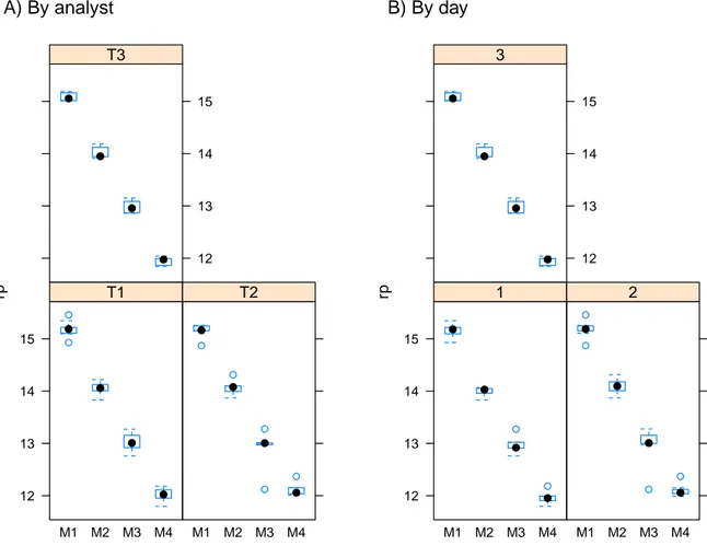
(34) 3.1. VALIDATION STUDY 1. 29. A) By analyst. B) By day. T1. 3 15. 15. 14. 14. 13. 13. 12. 12. T2. rp. rp. T3. 15. 15. 14. 14. 13. 13. 12. 12 M1 M2 M3 M4. M1 M2 M3 M4. 1. 2. M1 M2 M3 M4. M1 M2 M3 M4. Figure 3.1: Boxplot of raw data by grouping factor analyst (A) or day (B). represent a random selection of all the days and analysts that could have been chosen and the main research question is weather there is a substantial amount of variation in the response that could be explained by their inclusion in a model. The goal of a validation study is to uncover the lack of robustness of an assay by controlling for known sources of variation that constitute the grouping factors, thus the ideal outcome is to find out a non substantial contribution of this factors to the overall variance. As it can be seen from the by-grouping-factor box plots in Figure 3.1, there is not a dramatic variation in the response attributable to any of the factors, at least that can be easily revealed by simple plotting. Apart from deciding which variable effects will be specified as fixed or random, the main difficulty at the beginning of the analysis is to uncover the relationship existing between factors (crossing, partial crossing or nesting). This property is not defined by the model one would like to fit but instead is an inherent property to the design itself. The use of level plots, such as the ones displayed in Figure 3.2, is a helpful tool to uncover the underlying relationship in the data. Panel A of Figure 3.2 reveals some interesting features. A plot showing only squares in the diagonal but not in the off-diagonal positions would be an indicative of a nesting relationship between factors, this is, levels of the nested factor (e.g. analyst) happens exclusively at one level of the parent factor.