Subspaces
L.A. Garc´ıa-Escudero, A. Gordaliza, C. Matr´an and A. Mayo-Iscar
AbstractGrouping around affine subspaces and other types of manifolds is receiv-ing a lot of attention in the literature due to its interest in several application fields. Allowing for different dimensions is needed in many applications. This work ex-tends the TCLUST methodology to deal with the problem of grouping data around different dimensional linear subspaces in the presence of noise. Two ways of con-sidering error terms in the orthogonal of the linear subspaces are considered.
Key words: Clustering, linear subspaces, dimensions, robustness.
1 Introduction
Many non-hierarchical clustering methods are based on looking for groups around underlying features. For instance, the well-knownk-means method creates groups aroundkpoint-centers. However, clusters found in a given data set are sometimes due to the existence of certain relationships among the measured variables.
On the other hand, the Principal Components Analysis method serves to find global correlation structures. However, some interesting correlations are non-global since they may be different in different subgroups of the data set even being the distinctive characteristic of groups. This idea has also been proposed with the aim
L.A. Garc´ıa-Escudero
Universidad de Valladolid, Facultad de Ciencias, Prado de la Magdalena S/N, 47011, Valladolid, Spain, e-mail: lagarcia@eio.uva.es
A. Gordaliza
Universidad de Valladolid, e-mail: alfonsog@eio.uva.es
C. Matr´an
Universidad de Valladolid, e-mail: matran@eio.uva.es
A. Mayo-Iscar
Universidad de Valladolid, e-mail: agustinm@eio.uva.es
to overcome the “curse of dimensionality” trouble in high-dimensional problems by considering that the data do not uniformly fill the sample space and that data points are indeed concentrated around low dimensional manifolds.
There exist many references about clustering around affine subspaces with equal dimensions within the statistical literature (see, e.g., [10] and [6] and the references therein). We can distinguish between two different approaches: “clusterwise regres-sion” and “orthogonal residuals methods”. In clusterwise regression techniques, it is assumed the existence of a privileged response or outcome variable that want to be explained in terms of the explicative ones. Throughout this work, we will be assum-ing that no privileged outcome variables do exist. Other model-based approaches have been already proposed based on fitting mixtures of multivariate normals as-suming that the smallest groups’ covariances eigenvalues are small (see, e.g, [3]) but they are not directly aimed at finding clusters around linear subspaces (see [10]).
It is not difficult to find problems where different dimensionalities appear. In fact, this problem has been already addressed by the Machine Learning community. For instance, we can find approaches like “projected clustering” (PROCLUS, ORCLUS, DOC,k-means projective clustering), “correlation connected objects” (4C method), “intrinsic dimensions”, “Generalized PCA”, “mixture probabilistic PCA”, etc.
We will propose in Section 2 suitable statistical models for clustering around affine subspaces with different dimensions. They come from extending the TCLUST modeling in [5]. The possible presence of a fractionαof outlying data is also taken into account. Section 3 provides a feasible algorithm for fitting them. Finally, Sec-tion 4 shows some simulaSec-tions and a real data example.
2 Data models
Clustering around affine subspaces: We assume the existence ofk feature affine subspaces in Rp denoted by Hj with possible different dimensionsdj satisfying
0≤dj≤p−1 (a single point ifdj=0). Each subspaceHjis so determined from
dj+1 independent vectors. Namely, a group “center”mj where the subspace is
assumed to pass through and dj unitary and orthogonal vectors ulj, l=1, ...,dj,
spanning the subspace. We can construct ap×djorthogonal matrixUjfrom theseulj
vectors such that each subspaceHjmay be finally parameterized asHj≡ {mj,Uj}.
We assume that an observation x belonging to the j-th group satisfies x=
PrHj(x) +ε∗j,with PrHj denoting the orthogonal projection ofxonto the subspace Hjgiven by PrHj(x) =mj+UjU′j(x−µj)andε∗j being a random error term chosen
in the orthogonal of the linear subspace spanned by the columns ofUj. Ifεjis a
ran-dom distribution inRp−dj, we can choseε∗
j =U⊥j εjwithUj⊥being a p×(p−dj)
orthogonal matrix whose columns are orthogonal to the columns ofUj(the
Gram-Schmidt procedure may be applied to obtain the matrixUj⊥). We will further assume thatεjhas a(p−dj)-elliptical distribution with density|Σj|−1/2g(x′Σ−j1x).
Given a data set{x1, ...,xn}, we define the clustering problem through the
k
∑
j=1i∈
∑
Rjlog(pjf(xi;Hj,Σj)), (1)
with∪kj=1Rj={1, ...,n},Rj∩Rl=/0 for j̸=land
f(xi;Hj,Σj) =|Σj|−1/2g
(
(xi−PrHj(xi))
′U⊥
j Σ−j 1(U⊥j )′(xi−PrHj(xi)) )
. (2)
Furthermore, we are assuming the existence of some underlying unknown weights pj’s which satisfy∑kj=1pj=1 in (1). These weights help to do more logical
assign-ments to groups when they overlap.
Robustness:The term “robustness” may be used in a twofold sense. First, in Ma-chine Learning, the term “robustness” is often employed to refer to procedures which are able to handle certain degree of internal within-cluster variability due, for instance, to measurement errors. This meaning obviously has to do with the consideration of data models as those previously presented. Another meaning for the term “robustness” (more common in the statistical literature) has to do with the ability of the procedure to resist to the effect of certain fraction of “gross errors”. The presence of gross errors is unfortunately the rule in many real data sets.
To take into account gross errors, we can modify the “spurious-outliers model” in [4] to define a unified suitable framework when considering these two possible meanings for the term “robustness”. Starting from this “spurious-outliers model”, it makes sense to search for linear affine subspacesHj, group scatter matricesΣj
and a partition of the sample∪kj=0Rj={1,2, ...,n}withRj∩Rl=/0 for j̸=land
#R0=n−[nα]maximizing the “trimmed classification log-likelihood”:
k
∑
j=1i∈
∑
Rjlog(pjf(xi;Hj,Σj)). (3)
Notice that the fractionα of observations inR0is not longer taken into account in
(3).
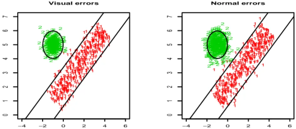
Visual and normal errors:Although several error terms may be chosen under the previous general framework, we focus on two reasonable and parsimonious distri-butions. They follow from consideringΣj=σjIp−dj and the followinggfunctions in (2):
a) Visual errors model(VE-model): We assume that the mechanism generating the errors follows two steps. First, we randomly choose a vector v in the sphere Sp−dj ={x∈R
p−dj:∥x∥=1}. Afterward, we obtain the error termε
jasεj=v· |z|withzfollowing aN1(0,σ2j)distribution. We call them “visual” errors because
we “see” (when p≤3) the groups equally scattered when theσj’s are equal independently of the dimensions. The VE-model leads to use:
f(x;Hj,σj) = (4)
= Γ
(
(p−dj)/2
)
π(p−dj)/2 √
2πσ2j
∥x−PrHj(x)∥
−(p−dj−1)/2exp(− ∥x−Pr
Hj(x)∥
2/2σ2
j
)
To derive this expression, consider the stochastic decomposition of a spherical distributionXinRp−dj asX=RUwithRa “radius” variable andUan uniform distribution onSp−dj. Ifhdenotes the p.d.f. ofRandgthe density generator of the
spherical family thenh(r) =Γ2((πp(p−−dd j)/2
j)/2)r
(p−dj)−1g(r2).Thus, ifR=|Z|withZ
being aN(0,1)random variable, we geth(r) =2/√2π·exp(−x2/2). Expression (4) just follows from (2). Notice thatg(x) =Cp−djx
N−1exp(−rxs)withN−1= −(p−dj−1)/2,r=1/2>0,s=1>0 (and satisfying the condition 2N+p>2).
Therefore, this density reduces to the univariate normal distribution whenever p−dj=1 and, in general, belongs to the symmetric Kotz type family [8].
b) “Normal” errors model(NE-model): With this approach, the mechanism gener-ating the error terms is based on adding a normal noise in the orthogonal of the feature spaceHj. I.e., we takeεjfollowing aNp−dj(0,σ
2
jIp−dj)distribution:
f(x;Hj,σj) = (2πσ2j)−(p−dj)/2exp
(
− ∥x−PrHj(x)∥
2/2σ2
j
)
(5)
The use of “normal” errors has been already considered in [1] and “visual” er-rors in [9] when working with 2-dimensional data sets and grouping around (1-dimensional) smooth curves.
Fig. 1 shows two generated data sets with VE- and NE-models. It also shows the boundaries of sets{x:d(x,Hj)≤z0.025/2}withz0.025being the 97.5% percentile
of theN1(0,1)andd(x,H) =infy∈H∥x−y∥whenH1is a point (a ball) and when
H2is a line (a “strip”). Note the great amount of observations that fall outside the
ball in the normal errors case although we had considered the same scatters in both groups. 1 1 1 1 1 1 1 1 1 1 1 1 1 1 1 1 1 1 1 1 1 1 1 1 1 1 1 1 1 1 1 1 1 1 1 1 1 1 1 1 1 1 1 1 1 1 1 1 1 1 1 1 1 1 1 1 1 1 1 1 1 1 1 1 1 1 1 1 1 1 1 1 1 1 1 1 1 1 1 1 1 1 1 1 1 1 1 1 11 1 1 1 1 1 1 1 1 1 1 1 1 1 1 1 1 1 1 1 1 1 1 1 1 1 1 1 1 1 1 1 1 1 1 1 1 1 1 1 1 1 1 1 1 1 1 1 1 1 11 1 1 1 1 1 1 1 1 1 1 1 1 1 1 1 1 1 1 1 1 1 1 1 1 1 1 1 1 1 1 1 1 1 1 1 11 1 1 1 1 1 1 1 1 1 1 1 1 1 1 1 1 1 1 11 11 1 1 1 1 1 1 1 1 1 1 1 1 1 1 1 1 1 1 1 1 1 1 1 1 1 1 1 1 1 1 1 1 1 1 1 1 1 1 1 1 1 1 1 1 1 1 1 1 1 1 1 1 1 1 1 1 1 1 1 1 1 1 1 1 1 1 1 1 1 1 1 1 1 1 1 1 1 1 1 1 1 1 1 1 1 1 1 1 1 1 1 1 1 1 1 1 1 1 1 1 1 1 1 1 1 1 1 1 1 1 1 1 1 1 1 1 1 1 1 1 1 1 1 1 1 1 1 1 1 1 1 1 1 1 1 1 1 1 1 1 1 1 1 1 1 1 1 1 1 1 1 1 1 1 1 1 1 1 1 1 1 1 1 1 1 1 1 1 1 1 1 1 1 1 1 1 1 1 1 1 1 1 1 1 1 1 1 1 1 1 1 1 1 1 1 1 1 1 1 1 1 1 1 1 1 1 1 1 1 1 1 1 1 1 1 1 1 1 1 1 1 1 1 1 1 1 1 1 1 1 1 1 1 1 1 1 1 1 1 1 1 1 1 1 1 1 1 1 1 1 1 1 1 1 1 1 1 1 1 1 1 1 1 1 1 1 1 1 1 1 1 1 1 1 1 1 1 1 1 1 1 1 1 1 1 1 1 1 1 1 1 1 1 1 1 1 1 1 1 1 2 2 2 2 2 2 2 2 2 2 2 2 2 2 2 2 2 22 2 2 2 2 2 2 2 2 2 2 22 2 2 2 22
22 2 2 2 2 22 2 2 2 22 2 22 2 2 2 2 2 2 2 22 2 2 2 2 2 2 2 2 2 2 2 2 2 2 2 2 2 2 2 22 2 2 2 2 2 2 2 22 2 2 2 2 222 2 2 2 2 2 2 22 2 2 2 2 2 2 2 2 2 2 2 2222
2222 2 2 2 2 2 2 2 2 2 2 2 2 2 2 2 2 2 2 2 2 2 2 2 2 2 2 2 22 2 2 2 2 2 22 2 2 2 2 2 2 2 2222 2 2 2 2 2 2 2 2 2 2 2 2 2 2 2 2 2 2 2 2 2 2 2 2 2 2 22
2 2 2 2 2 2 2 2 2 2 2 2 2 2 2 2 2 2 2 2 2 2 22 222 2 2 2 2 2 2 2 2 2 2 2 2 2 22222
2 2 2 2 2 2 2 2 2 22 22 2 2 2 2 2 2 2 2 2 2 2 2 2 2 22 2 2 2 2 2 2 2 2 2 2 2 2 2 2 22 2 2 2 2 2 2 22 2 22 2 2 22 2 2 2 2 2 2 2 2 2 22 2 2 2 2 2 2 2 2 2 2 2 2 2 2 2 222 2 2 2 22 2 22 2 2 2 2 2222
2 2 2 2 2 2 2 2 2 2 22 2 2 2 2 2 222 2 222222222
2 2
22222 2 2 2 2 2 2 2 2 2 222 2 2 2 2 2 2 2 2 2 2 2 2 2 2 2 2
2222 2 2 22 2 2 2 2 22 2 2 2 22 222 222 2 2 2 2 2 2 2 2 2 2 22 2 2 2 2 2 2 2 2 2 2 2 2 22 2 2 2 2 2 2 2 2 2 2 2 22 2 2 2 2 222 2 2 2 2 22 2 2 22
2222
−4 −2 0 2 4 6
0 1 2 3 4 5 6 7 Visual errors 1 1 1 1 1 1 1 1 1 1 1 1 1 1 11 1 1 1 1 1 1 1 1 1 1 1 1 1 1 1 1 1 1 11 1 1 1 1 1 1 1 1 1 1 1 1 1 1 1 1 1 1 1 1 1 1 1 1 1 1 1 1 1 1 1 1 1 1 1 1 1 1 1 1 1 1 1 1 1 1 1 1 1 1 1 1 1 1 1 1 1 1 1 1 1 1 1 1 1 1 1 1 1 1 1 1 1 1 1 1 1 1 1 1 1 1 1 1 1 1 1 1 1 1 1 1 1 1 1 1 1 1 11 1 1 1 1 1 1 1 1 1 1 1 1 1 1 1 1 1 1 1 1 1 1 1 1 1 1 1 1 1 1 1 1 1 1 1 1 1 1 1 1 1 1 1 1 1 1 1 1 1 1 1 1 1 1 1 1 1 1 1 1 1 1 1 1 1 1 1 1 1 1 1 1 1 1 1 1 1 1 1 1 1 1 1 1 1 1 1 1 1 1 1 1 1 1 1 1 11 1 1 1 1 1 1 1 1 1 1 1 11 1 1 1 1 1 1 1 1 1 1 1 1 1 1 1 1 1 1 1 1 1 1 1 1 1 1 1 1 1 1 1 1 1 1 1 1 1 1 1 1 1 1 1 1 1 1 1 1 1 1 1 1 1 1 1 1 1 1 1 1 1 1 1 1 1 1 1 1 1 1 1 1 1 1 1 1 1 1 1 1 1 1 1 1 1 1 1 1 1 1 1 1 1 1 1 1 1 1 1 1 1 1 1 1 1 1 1 1 1 1 1 1 1 11 1 1 1 1 1 1 1 1 1 1 1 1 1 1 1 1 1 1 1 1 1 1 1 1 1 1 11 1 1 1 1 1 1 1 1 1 1 1 1 1 1 1 1 1 1 1 1 1 1 1 1 1 1 1 1 1 1 1 1 1 1 1 1 1 1 1 1 1 1 1 1 1 1 1 1 1 1 1 1 1 1 1 1 1 1 1 1 1 1 1 1 1 1 1 1 1 1 1 1 1 1 1 1 1 1 1 1 1 1 1 1 1 1 1 1 1 1 1 1 1 1 1 1 1 1 1 1 1 1 1 1 1 1 1 1 1 1 2 22 2 2 2 2 2 22 2 2 2 2 2 2 2 2 2 2 2 2 2 2 2 2 2 2 2 2 2 2 2 2 2 2 2 2 2 2 2 2 2 2 2 2 2 2 2 2 2 2 2 2 22 2 2 2 2 2 2 2 2 2 2 2 2 2 2 2 2 2 2 2 2 2 2 2 2 2 2 2 2 2 2 2 2 2 2 2 2 2 2 22 2 2 22 2 2 2 2 2 2 2 2 2 2 2 2 22 2 222
2 2 2 2 2 2 2 2 2 2 2 2 2 2 2 2 2 2 2 2 2 2 2 22 2 2
2 2 2 2 22 2 2 22 2 2 22 22 2 2 22 2 2 2 2 2 222 2 2 2 2 22 2 2 2 2 2 2 2 2 2 2 2 2 2 2 2 2 2 22 2 2 2 2 2 22 2 2 2 2 2 2 2 2 2 2 2 22 2 2 2 2 22 2 2 2 2 2 2 2 2 2 2 2 2 2 2 2 2 2 2 2 2 2 2 2 2 2 2 2 2 2 2 2 2 2 2 2 2 2 22 2 2 2 2 2 2 2 2 2 2 2 2 2 2 2 2 2 2 2 2 2 2 2 2 2 2 2 2 2 2 2 2 2 2 2 2 2 2 2 2222 2 2 2 22 2 2 22 2 2 2 2 2 2 2 2 2 2 2 2 2 2 2 2 2 2 2 2 2 2 2 2 2 2 2 2 2 2 22
2 2 2 22 2 2 2 2 2 2 2 2 2 2 2 2 2 2 22 2 2 2 2 2 2 2 2 2 2 2 2 2 2 2 2 2 2 2 22 2 22 2 2 2 2 2 2 2 2 2 2 2 2 2 22 2 2 2 2 2 2 2 2 2 2 2 2 2 2 2 2 2 22 2 2 2 2 2 2 2 2 2 2 2 2 2 2 2 2 2 2 2 2 2 2 2 2 2 222 2 2 2 2 2 2 2 2 2 2 2 2 2 2 2 2 2 2 2 2 2 2 2 2 2 2 2 2 2 2 2 2 2 2 2 2 2 2 2 2 2 2 2 2 2 2
−4 −2 0 2 4 6
0 1 2 3 4 5 6 7 Normal errors
Fig. 1 Simulated data set from the VE- and NE- models.
Constraints on the scatter parameters:Let us considerdj+1 observations andHj
WhenΣj=σjIp−dj, the constraints introduced in [5] are translated into
max
j σ
2 j
/ min
j σ
2
j ≤cfor a given constantc≥1. (6)
Constant cavoids non interesting clustering solutions with clusters containing very few almost collinear observations. This type of restrictions goes back to [7].
3 Algorithm
The maximization of (3) under the restriction (6) has high computational complex-ity. We propose here an algorithm inspired in the TCLUST one. Some ideas behind the classification EM algorithm [2] and from the RLGA [6] also underly.
1. Initialize the iterative procedure:Set initial weights values p01=...=p0k=1/k and initial scatter valuesσ0
1 =...=σk0=1. As startingklinear subspaces,
ran-domly selectksets ofdj+1 data points to obtainkinitial centersm0jandkinitial
matricesU0
j made up of orthogonal unitary vectors.
2. Update the parameters in the l-th iteration as:
2.1. Obtain
Di= max j=1,...,k{p
l
jf(xi;mlj,Ulj,σlj)} (7)
and keep the setRl with then−[nα]observations with largestDi’s. SplitRl
intoRl={Rl1, ...,Rlk}withRlj={xi∈Rl:pljf(xi;mlj,Ulj,σlj) =Di}.
2.2. Update parameters by using:
• plj+1←-“nlj/[n(1−α)]withnljequal to the number of data points inRlj”.
• mlj+1←-“The sample mean of the observations inRl j”.
• Ulj+1←-“A matrix whose columns are equal to thedjunitary eigenvectors
associated to the largest eigenvalues of the sample covariance matrices of observations inRlj”.
Use the sum of squared orthogonal residuals to obtain initial scatters s2j = 1
nl j∑xi∈R
l
j∥xi−PHlj(xi)∥
2withHl
j≡ {mlj,Ujl}. To satisfy the constrains, they
must be “truncated” as:
[s2j]t=
s2
j ifs2j∈[t,ct]
t ifs2j<t ct ifs2j>ct
. (8)
Search fortopt=arg maxt∑kj=1∑xi∈Rljlogf(xi;m
l+1
j ,Ulj+1,[s2j]t)and take • σl+1
j ←
-√
[s2
j]topt.
3. Compute the evaluation function:PerformLiterations of the process described in step 2 and compute the final associated target function (3).
Determiningtopt implies solving a one-dimensional optimization problem that
can be easily done by resorting to numerical methods. More details concerning the rationale of this algorithm can be found in [5]. We denote the previous algorithm as VE-method when the density (4) is applied and as NE-method when using (5).
4 Examples
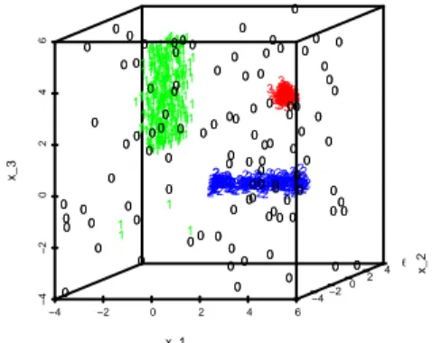
Simulation study:Let us consider a clustering problem where observations are gen-erated around a point, a line and a plane inR3. We generate uniformly-distributed points on the setsC1={(x1,x2,x3):x1=x2=x3=3} (no random choice), on
C2={(x1,x2,x3): 1≤x1≤6,x2=x3=3}, and, onC3={(x1,x2,x3):x1=−2,1≤
x2≤6,1≤x3≤6}. Later, we add error terms in the orthogonal of theCj’s
consid-ering the models introduced in Section 2. Finally, points are randomly drawn on the cube[−4,6]×[−4,6]×[−4,6]as “gross errors”. Fig. 2 shows the result of the proposed clustering approach for a data set drawn from that simulations scheme.
−4 −2 0 2 4 6
−4 −2 0 2 4 6 −4−2 0 2
4 6
x_1 x_2 x_3 0 1 0 0 0 0 0 0 0 1 1 1 0 1 1 1 1 1 1 1 1 1 1 1 1 1 1 1 1 1 1 1 1 1 1 11 0 1 1 1 1 1 1 11 1 1 1 1 1 1 11 1 1 1 1 1 1 1 1 11 1 1 1 1 1 0 1 1 1 11 1 1 11 1 1 1 1 1 11
1 111
1 0 1 1 1 11 0 1 1 11 1 1 1 1 1 1 1 1 1 1 1 1 11 1 1 1 1 1 0 11 0 1 1 1 1 1 1 1
111
0 1 1 1 1 1 1 1 1 1 1 1 1 1
1 111
1 1 1 1 1 1 0 3 1 11 1 1 0 3 1 1 1 1 1 11 1 1 1 3 1 1 1 1 1 1 3
1 333
0 3 1 3 3 3 3 1 1 1 3 1 3 3 1 1 0 3 1 3 3 3 1 1 1
3333 33
1 3333
1 1 3 3 3 33 1 1 1 3 1 3 33 33 1 3 1 3 1 3 33 1 1 3 1
3333333333 3 3 3 33 3 0 3 3 33 3333
1
3 3 33333
1
3 33
1
3 333333333333333
3
1
33
1 333333333333333333333333
1 3 3 3 3 3 33 333 33 33 3 3 333333333333333
0
1 3333
1
33
1
1
33 3333333
1 33 1 3 33 0 1 33 33 333333 333
1
33
1 3333
1
3
1 333
1 3 3 333 1 3 33 1 1 3 3 333 1 1 3 1 1 1 3 33 1 3 1 3 1 33 1 3 3 33 1 3 3 3 33 0 0 3 33 33 1 3 1 3 1 11 0
111
1 3 1 1 1 33 1 3 1 3 1 3 33 1 1 3 1 1 1 11 3 1 1 1 3 1 0 1 1 3 3 1 1 3 1 1 1 1 1 1 1 1 3 1 1 1 1 11 1 1 1 1 11 0 1 1 1 1 0 1 0 1 1 1 1 1 0 1 1 1 1 1 1 1 1 1 1 1 0 1 1 1 1 1 1 1 1 1 1 1 1 0 1 1 1 1 1 0 1 1 1 111 0 1 1 1 1 1 1 1 1 0 1 1
11 11
1 1 1 0 1 1 1 1 1 0 1 1 1 1 1 1 1 1 1 1 1 0 0 1 1 0 1 1 1 1 1 1 1 1 1 1 1 1 1 1 10 1 0 1 1 1 1 1 1 1 1 1 1 1 1 0 1 0 1 1 1 1 0 0 1 1 1 1 1 1 1 1 1 1 1 1 1 1 1 1 1 1 1 1 1 0 0 0 0 0 0 2
2 222222 2 2 2 2
22 2 222 2 2222
2 2 2 2 22 22 2
2 2 22222 2222 222222 22222
2 22 2
2 2 2 22 22 2222
0 2
0
22 22 2 2 2 2 2 2 2 22
22 2 2
222 22 2 0 2 2 0 22 2 222 2 2
2 22 22 2 2 2 22 2222 2222 2 2222222222222222222222 22222 2222222222222 0
2 2 2 222 2
2 2 2 2 2
2 2 2 2 2222 2 2
2 2 22 2 22 2 22 2 2 2 2222 2 22 222222222 2 22222 2 2 22 0 2 2 2 0 2 22 2 2 0 2 2 2 22 2 22 22 22
2 2 2 0 0 0 0 1 0 0 0 0 0 0 1 0 0 0 0 0 0 0 0 0 0 0 0 0 0 0 0 0 0 0 0 0 0 0 0 0 0 0 0 0 0 0 0 0 0 0 0 0 0 0 0 0 0 0 0 0 0 0 0 0 0 0 0 0 0 0 0 0 0 0 0 0 0 0 0 0 0 0 0 0 0 0 0 0 0 0 0 0 0 0 0 0 0 0 0 0 0 0 0 0 0 0 0 0 0 0 0 0 0 0 0 0 0 0 0 0 0 0 0 0 0 0 0 0 0 0 0 0 0 0 0 0 0 0 0 0 0 0 0 0
Fig. 2 Result of the NE-method withk=3,dj’s= (0,1,2),c=2 andα=.1.
A comparative study based on the previous simulation scheme with VE- and NE-methods has been carried out. We have also considered an alternative (Euclidean distance) ED-method where theDi’s in (7) are replaced by the more simple
ex-pressionsDi=infj=1,...,k∥xi−PHl
j(xi)∥and no updating of the scatter parameters is done. The ED-method is a straightforward extension of the RLGA in [6].
0 200 400 600 800 1000
0.00
0.15
0.30
(a) Data from VE−model and L = 5
Number of initializations S
prop. missclasif.
VE− NE− ED−
0 200 400 600 800 1000
0.00
0.15
0.30
(b) Data from NE−model and L = 5
Number of initializations S
prop. misclassif.
VE− NE− ED−
0 200 400 600 800 1000
0.00
0.15
0.30
(c) Data from VE−model and L = 10
Number of initializations S
prop. misclassif.
VE− NE− ED−
0 200 400 600 800 1000
0.00
0.15
0.30
(d) Data from NE−model and L = 10
Number of initializations S
prop. misclassif.
VE− NE− ED−
0 200 400 600 800 1000
0.00
0.15
0.30
(e) Data from VE−model and L = 20
Number of initializations S
prop. misclassif.
VE− NE− ED−
0 200 400 600 800 1000
0.00
0.15
0.30
(f) Data from NE−model and L = 20
Number of initializations S
prop. misclassif.
VE− NE− ED−
Fig. 3 Proportion of misclassified observations in the simulation study described in the text.
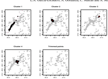
Real data example:As in [9], we consider position data on some earthquakes in the New Madrid seismic region from the CERI. We include all earthquakes in that cat-alog from 1974 to 1992 with magnitude 2.25 and above. Fig. 4 shows a scatter plot of the earthquakes positions and a nonparametric kernel based density estimation suggesting the existence of a linear tectonic fault and three main point focuses.
35.5 36.5 37.5
−91.0
−90.5
−90.0
−89.5
−89.0
−88.5
New Madrid data
Longitude
Latitude
35.5 36.0 36.5 37.0 37.5 38.0
−90.5
−90.0
−89.5
−89.0
−88.5
Longitude
Latitude
Fig. 4 Earthquake positions in the New Madrid seismic region.
35.5 36.5 37.5
−91.0
−90.5
−90.0
−89.5
−89.0
−88.5
Cluster 1
35.5 36.5 37.5
−91.0
−90.5
−90.0
−89.5
−89.0
−88.5
Cluster 2
x
35.5 36.5 37.5
−91.0
−90.5
−90.0
−89.5
−89.0
−88.5
Cluster 3
x
35.5 36.5 37.5
−91.0
−90.5
−90.0
−89.5
−89.0
−88.5
Cluster 4
x
35.5 36.5 37.5
−91.0
−90.5
−90.0
−89.5
−89.0
−88.5
Trimmed points
Fig. 5 Clustering results of the VE-method fork=4,dj’s= (1,0,0,0),c=2 andα=.4.
5 Future research directions
The proposed methodology needs to fix parameters k,dj’s,α andc. Sometimes
they are known in advance but other times they are completely unknown. “Split and merge”, BIC and geometrical-AIC concepts could be then applied. Another important problem is how to deal with remote observations wrongly assigned to higher dimensional linear subspaces due to their “not-bounded” spatial extension. A further second trimming or nearest neighborhood cleaning could be tried.
References
1. Banfield, J.D. and Raftery, A.E. (1993) “Model-based Gaussian and non-Gaussian clustering”.
Biometrics,49, 803–821.
2. Celeux, G. and Govaert, A. (1992). “Classification EM algorithm for clustering and two stochastic versions”.Comput. Statit. Data Anal.,13, 315-332.
3. Dasgupta, A. and Raftery, A.E. (1998) “Detecting features in spatial point processes with clutter via model-based clustering.”J. Amer. Statist. Assoc.,93, 294-302.
4. Gallegos, M.T. and Ritter, G. (2005), “A robust method for cluster analysis,”Ann. Statist.,33, 347-380.
5. Garc´ıa-Escudero, L.A., Gordaliza, A., Matr´an, C. and Mayo-Iscar, A. (2008a). “A general trimming approach to robust clustering”,Ann. Statist.,36, 1324-1345.
6. Garc´ıa-Escudero, L.A., Gordaliza, A., San Mart´ın, R., Van Aelst, S. and Zamar, R. (2008b). “Robust Linear Grouping”.J. Roy. Statist. Soc. B,71, 301-319.
7. Hathaway, R.J. (1985), “A constrained formulation of maximum likelihood estimation for normal mixture distributions,”Ann. Statist,13, 795-800.
8. Kotz, S., 1975. “Multivariate distributions at a cross-road”. InStatistical Distributions in Sci-entific Work, G.P. Patil, S. Kotz, J.K. Ord, eds.,1, 247270.
9. Standford, D.C. and Raftery, A.E. (2000). “Finding curvilinear features in Spatial point pat-terns: Principal Curve Clustering with Noise”.IEEE Trans. Pattern Recognition,22, 601-609. 10. Van Aelst, S., Wang, X., Zamar, R. H. and Zhu, R. (2006) “Linear grouping using orthogonal