Preprint of the paper
"A Boundary Element Numerical Approach for Earthing Grid Computation"
I. Colominas, F. Navarrina, M. Casteleiro (1999)
Computer Methods in Applied Mechanics & Engrng., 174 , 73-90.
Grounding Grid Computation
I. Colominas, F. Navarrina, M. Casteleiro
Dpto. de Metodos Matematicos yde Representacion,E.T.S.de Ingenierosde
Caminos, Canalesy Puertos;Universidad de La Coru ~na. Campus de Elvi ~na,
15192 La Coru ~na, SPAIN
Abstract
Analysis anddesign of substationearthinginvolvescomputing theequivalent
re-sistance of grounding systems, as well as distribution of p otentials on the earth
surfacedue tofault currents[1,2].While very crudeapproximations wereavailable
in the sixties, several metho ds have b een prop osed in the last two decades, most
of them on the basis of intuitive ideas such as sup erp osition of punctual current
sources and error averaging [3,4].Although these techniques represented a
signi-cantimprovementintheareaofearthinganalysis, anumb erofproblemshave b een
rep orted; namely: large computational requirements, unrealistic results when
seg-mentation of conductors is increased, and uncertainty in the margin of error [4].
A Boundary Element approach for the numerical computation of substation
groundingsystemsispresentedin thispap er.Severalwidespreadintuitive metho ds
(such as theAverage Potential Metho d) can b e identied in this general
formula-tion as the result of suitable assumptions intro duced in the BEM formulation to
reduce computational cost for sp ecic choices of the test and trial functions. On
theotherhand,thisgeneralapproachallowstheuseoflinearandparab olicleakage
current elements toincrease accuracy. Eortshave b een particularly made in
get-ting a drastic reduction in computing timebymeans of newcompletely analytical
integrationtechniques, whilesemi-iterative metho dshaveproventob esp eciall y
ef-cient forsolving the involved system of linear equations. This BEM formulation
has b een implemented in a sp ecic Computer Aided Design system for grounding
analysis develop ed within the last years. The feasibility of this approach isnally
1.1 Mathematical Model of the Physical Problem
A safe earthing system has to guarantee the integrity of equipment and the
continuityoftheserviceunderfaultconditions|providingmeanstocarryand
dissipate electricalcurrents into the ground| and to safeguard that p ersons
working or walking in the surroundings of the grounded installation are not
exp osed to dangerous electricalsho cks. To achievethese goals, the equivalent
electrical resistance of the system must b e low enough to assure that fault
currents dissipate mainly through the grounding grid into the earth, while
maximump otentialdierencesb etweenclosep ointson theearthsurfacemust
b e kept under certaintolerances (step, touchand meshvoltages) [1,2].
Physical phenomena underlying fault currents dissipation into the earth can
b emo delledby meansof Maxwell'sElectromagneticTheory[5].Constraining
the analysis to electrokinetic steady-state resp onse [1,6], and neglecting the
inner resistivity of the earthing electro de (a system of interconnected buried
conductors), the 3D problem asso ciated with an electricalcurrent derivation
to earth can b e written as
div() =0; =0grad(V) in E;
V =V
0
in 0; nnnnnnn
n n n n n n n E
1
=0 in 0
E
: (1)
where E is the earth,
its conductivity tensor, 0
E
the earth surface, nnnnnnnnnn
n n n n E
its
normal exterior unit eld and 0 the electro de surface [7,8]. The solution to
this problem givesthe p otential V and the currentdensity at an arbitrary
p oint xxxxxxx
x x x
xx
x
x when the electro de attains a voltage V
0
(Ground Potential Rise or
GPR) relativeto adistantgrounding p oint assumedto b e at the p otential of
remote earth.
Intheseterms,b eingnnnnnnnnnn
n n n n
thenormalexterioruniteld to0,the leakage current
density at an arbitrary p oint of the earthing electro de surface, the ground
currentI
0
(totalsurgecurrentb eing leakedinto theearth)andthe equivalent
resistance of the earthing system R
eq
(apparent resistance of the electro
de-earth circuit)can b ewritten as
=
t
n n n n
nnn
n n n
nn
n
n; I
0 =
Z Z
0
d0; R
eq =
V 0
I 0
: (2)
For most practical purp oses, the assumption of homogeneous and isotropic
soil can b e considered accurate [2], and the tensor
can b e substituted by
kindof techniquesdescrib edin this pap er can b e extendedto multi-layersoil
mo dels[9,20](representingthe ground as stratied into twoor morelayersof
appropriatethickness,eachone withadierentvalue of),furtherdiscussion
andexamplesarerestrictedtouniformsoilmo dels.Hence,problem(1)reduces
to the Laplaceequation with mixedb oundary conditions [5].
Onthe otherhand,if onefurtherassumesthatthe earthsurfaceishorizontal,
symmetry(metho dofimages)allowsustorewrite(1)intermsoftheDirichlet
Exterior Problem:
1V = 0 in E
V = V
0
in 0 and 0
0
(3)
where the image surface 0
0
is the symmetric of 0 with resp ect to the earth
surface [7,8]. The assumption of horizontal earth surface seems to b e quite
adequate,if we considerthat surroundings of almost every electrical
installa-tionmustb eleveledb eforeitsconstruction.FurtherassumptionV
0
=1isnot
restrictiveat all,since V and are prop ortionalto V
0 .
2 Variational Statement of the Problem
In most electrical installations, the earthing electro de consists of a grid of
interconnected bare cylindrical conductors, horizontally buried and
supple-mentedbyanumb erofverticalro ds, whichratiodiameter/lengthisrelatively
small(10
03
).Obviously,noanalyticalsolutionscanb eobtainedforthiskind
of problem. Moreover, this sp ecic geometry precludes the use of standard
numericaltechniques(suchas FiniteDierencesor FiniteElements[11]) since
discretization of domain E is required, and obtaining suciently accurate
results should imply unacceptable computing eorts in memory storage and
cpu time.
However,computation of p otential is only required on the earth surface and
the equivalent resistance can b e easily obtained (2) in terms of the current
density that leaks from the electro de surface. Thus, we turn our attention
to a Boundary Integral approach, whichwould only require discretization of
the earthing grid surface 0, and will therefore reduce the three-dimensional
problemto atwo-dimensionalone.
Applicationof Green'sIdentity[12,13]to (1)allows usto obtainthefollowing
V(xxxxxxxxxx x x x
x)=
1
4
Z Z
20
k(xxxxxxxxxx
xx
x
x;
)(
)d0; (4)
with the weakly singular kernel
k(xxxxxxx
xxx
x x x
x;
) =
1
r (xxxxxxxxxx
xx
x
x;
)
+ 1
r (xxxxxxxxxx x x x
x;
0
) !
; r (xxxxxxx
x x x x x x
x;
) = jxxxxxxx
x x x x x x
x0
j; (5)
where
0
0
0
0
0
0
0
0
0
0
0
0
0
0
is the symmetricof with resp ect to the earthsurface [7,8].
Since (4) holds [8] on the earthing electro de surface 0 and the p otential is
known bytheb oundarycondition ontheGPR(V(
)=1;
20),the leakage
currentdensity mustsatisfythe Fredholmintegralequationofthe rstkind
denedon 0
1 =
1
4
Z Z
20
k(
;
) (
)d0;
20: (6)
Finally,a weaker variational form[10] of equation (6) can now b e writtenas:
Z Z
20
w (
)
"
10
1
4
Z Z
20
k(
;
)(
)d0
#
d0=0; (7)
which must hold for all memb ers w (
) of a suitable class of test fuctions
denedon 0.
Obviously,aBoundaryElementapproachseemstob etherightchoiceto solve
variational statement(7).
2.1 Boundary Element Formulation
ForagivensetofN trialfunctionsfN
i (
)gdenedon 0,andforagivensetof
M 2D b oundary elementsf0
g, the unknown leakage current density and
the earthing electro de surface 0 can b e discretizedin the form
(
)=
N X
i=1
i N
i
(
); 0=
M [
=1 0
V(xxxxxxxxxx x x x
x)=
N X
i=1
i V
i (xxxxxxxxxx
xx
x
x); V
i (xxxxxxxxxx
xx
x
x)=
M X
=1 V
i
(xxxxxxxxxx x x x
x); (9)
V i
(xxxxxxxxxx x x x
x)=
1
4
Z Z
20
k(xxxxxxxxxx
xx
x
x;
)N
i
(
) d0
: (10)
Moreover,for a givenset of N test functions fw
j
()g dened on 0, the
vari-ational statement(7) is reducedto the systemof linear equations
N X
i=1 R
ji
i
=
j
; j =1;:::;N; (11)
R ji
= M X
=1 M X
=1 R
ji
;
j =
M X
=1
j
; (12)
R ji
= 1
4
Z Z
20
w
j
()
Z Z
20
k(; ) N
i
() d0
d0
(13)
j
=
Z Z
20
w
j
(
)d0
: (14)
Inpractice,the 2Ddiscretizationrequiredtosolvetheab ove statedequations
inreal problemsimplies an extremelylarge numb erof degrees of freedom.In
addition ifwetakeintoaccountthat theco ecientsmatrixin(11) isfulland
the computation of each contribution (13) requires double integration on 2D
domains,weconcludethatsomeadditionalsimplicationsmustb eintro duced
to overcomethe extremelyhigh computationalcost ofthe problem.
3 Approximated 1D Variational Statement
With this scop e, and considering the characteristic geometry of grounding
grids in most of real electricalinstallations, one can assume that the leakage
currentdensityisconstantaroundthecrosssectionofthecylindricalelectro de
[7,8]. This hyp othesis of circumferentialuniformity is widely used in most of
thetheoreticaldevelopmentsand practicaltechniquesrelatedintheliterature
[1,2,4].
LetLb ethewholesetofaxiallinesoftheburiedconductors,
b
the orthogonal
projection overthe bar axisof a givengeneric p oint
20, (
b
) the electro de
diameter, C(
b
) the circumferential p erimeter of the cross section at
b
b (
)theapproximatedleakagecurrentdensityatthis p oint(assumeduniform
around the cross section).Thus, expression(4) can b ewritten in the form
b
V(xxxxxxxxxxxxxx)=
1 4 Z b 2L " Z 2C( b )
k(xxxx;xxxxxxxxxx ) dC
# b ( b
)dL: (15)
Now,since theleakagecurrentisnot exactlyuniformaroundthecrosssection,
b oundary condition V(
) = V
0 = 1;
2 0 will not b e strictly satised at
everyp oint
on the electro desurface 0,and variational equality(7) willnot
holdanymore.However,ifwerestrictthe class oftrialfunctionsto those with
circumferentialuniformity,that isw (
)= b w (b ) 8 2 C(b
),(7) resultsin:
Z b 2L b w(b ) " ( b )0 1 4 Z b 2L K( b ; b ) b ( b )dL #
dL=0 (16)
which must hold for all memb ers
b w( b
) of a suitable class of test fuctions
denedon L, b eing the integral kernel
K( b ; b )= Z 2C(b ) " Z 2C( b ) k( ; )dC #
dC : (17)
Inthisway,the b oundaryconditionhastob esatisedonthe averageatevery
crosssection.Infact,(16)canb econsideredasaweakervariationalstatement
of the Fredholmintegralequation of the rst kindon L
( b )= 1 4 Z b 2L K(b ; b ) b ( b
)dL 8
b
2L: (18)
Since ends and junctions of conductors are not taken into account in this
formulation,slightly anomalous lo caleects are exp ectedat these p oints,
al-though global results should not b e noticeablyaected inreal problems.
3.1 1D BoundaryElement Formulation
Resolution of integral equation (16) involves discretization of the domain
formed by the whole set of axial lines of the buried conductors L. Thus, for
givensets of n trial functions f
c N i ( b
)g dened on L, and m 1D b oundary
el-ements fL
g, the unknown approximated leakage current density
b
and the
setof axial linesLcan b e discretizedinthe form
b ( b )= n X i=1 b i c N i ( b
); L=
as
b
V(xxxxxxx
x x x x x x x)= n X i=1 b i b V i
(xxxxxxx x x x xx x x); b V i
(xxxxxxx x x x xx x x)= m X =1 b V i
(xxxxxxx
xxx
x x x x); (20) b V i
(xxxxxxxxxx x x x x)= 1 4 Z b 2L " Z 2C( b )
k(xxxxxxxxxx
xx x x; )dC # c N i ( b
) dL: (21)
Finally, for a suitable selection of n test functions f
b w j ( b
)g dened on L,
equation (16) isreduced to the system of linearequations
n X i=1 b R ji b i = b j
; j =1;:::;n; (22)
b R ji = m X =1 m X =1 b R ji ; b j = m X =1 c j ; (23) b R ji = 1 4 Z b 2L b w j (b ) Z b 2L K(b ; b ) c N i ( b )dL dL; (24) b j = Z b 2L ( b ) b w j (b
) dL: (25)
On a regular basis, the computational work required to solve a real problem
isdrasticallyreducedby meansof this 1Dformulationwith resp ect to the2D
formulationgiveninsection2,mainlyb ecausethe sizeof the linearequations
system(22)andthenumb erofcontributions(24)thatisnecessarytocalculate
are exp ectedto b e signicantlysmaller than those in(11) and (13).
However,extensivecomputing isstillrequired for integration. Since integrals
onthecircumferentialp erimeterofelectro desaretakenseparatefromintegrals
on theiraxiallines,welo okforward to reducingthe highcomputationaleort
required for circumferential integration in (17) and (21). Obviously, further
simplicationsarenecessaryto reducecomputingtimeunderacceptablelevels
[8].
3.2 Simplied 1D Boundary Element Formulation
The inner integral of kernel k(xxxxxxx
x x x xx x x;
) in (21) can b e writtenas:
Z 2C( b )
k(xxxxxxxxxx x x x x;
)dC =
Z 2C( b ) 1
r (xxxxxxxxxx
xx x x; ) dC+ Z 2C( b ) 1
r (xxxxxxxxxx x x x x; 0 )
Distance r (xxxxxxxx;xxx ) b etween any p ointxxxxxxxxxxx in the domainand an arbitrary p oint
at the earthing electro desurface can b e expressedas:
r (xxxxxxxxxx
xx x x; )= s
jxxxxxxxxxx x x x x 0 b j 2 + 2 ( b ) 4
0jxxxxxxxxxx
xx x x 0 b j( b
) sin! cos (27)
where isthe angular p osition in the p erimeterof cross section of the
cylin-drical conductor, and
sin! =
j( b
0xxxxxxx
x xx x x x x) 2 b s s s s
sss
s s s ss s s( b )j j b
0xxxxxxxxxx x x x x j (28)
as shown ingure 1.
The ellipticintegralobtained when r (xxx;xxxxxxxxxxx ) in (27)is substitutedinto (26)can
b e approximated by means of numericalintegration up to an arbitrary level
ofaccuracy. However,since weareinterestedincomputingp otentialat p oints
x x x
xxxx
x x x x x x
x on the earth surface, whichdistanceto arbitraryp oints
b
on the axial lines
is much larger that the diameter (
b
) of the earthing electro de [8], distance
r (xxxx;xxxxxxxxxx ) in (27) can b e approximatedas
r (xxxxxxxxxx
xx x x; ) b r (xxxxxxxxxx
xx x x; b ) = s
jxxxxxxxxxx x x x x 0 b j 2 + 2 ( b ) 4 : (29)
Then, the inner integral of kernelk(xxxxxxx
xxx
x x x x;
) in (26) can b eapproximatedas:
Z 2C( b )
k(xxxx;xxxxxxxxxx ) dC (
b ) b k(xxxxxxxxxxxxxx;
b ); (30) where b k(xxxxxxxxxxxxxx;
b )= 0 @ 1 b
r (xxxxxxx
x x x xx x x; b ) + 1 b r(xxxxxxxxxx
xx x x; b 0 ) 1 A : (31) and b 0
is the symmetric of
b
with resp ect to the earth surface. Expression
(30) can b e interpretedas the result of applying aNewton-Cotes cuadrature
withonesinglep ointto (26).Thisapproximationwillb equiteaccurateunless
distanceb etweenp ointsxxxxxxx
xxx
x x x xand b
isofthe sameorderofmagnitudeasdiameter
( b
),whichwill not o ccur if this approximation isused to computep otential
(ξ)
ξ
ξ
θ
ω
Fig.1. Distanceb etween agiven p oint xxxxxxxxxxxxxx and anarbitrary p oint atthe electro de
surface.
Substituting(30) into (17), we can approximate:
K( b ; b ) Z
2C(b)
( b ) b k( ; b
)dC : (32)
Next, b earing in mind once again the approximations used in (29), integral
kernel (17) can now b esimplied as:
K( b ; b ) ( b )( b ) b b k(b ; b ); (33) b eing b b k(b ; b ) = 0 @ 1 b b r( b ; b ) + 1 b b r ( b ; b 0 ) 1 A ; (34) and b b r ( b ; b ) = s j b 0 b j 2 + 2 ( b )+ 2 ( b ) 4 ; (35)
where inclusion of b oth diameters (
b
) and (
b
) authomatically preserves
the symmetry in the system of equations (22) although the conductor cross
sectionsweredierentat p oints
b and b .
Now,dierentselectionsofthe setsof trialandtest functionsin(24)and(25)
allow us to obtain sp ecic formulations. Thus, for constant leakage current
elements(onecenteredno dep ersegmentofconductor),PointCollo cation
sphere".Ontheotherhand,Galerkintyp eweighting(wheretest functionsare
identical to trial functions) leads to a kind of morerecent metho ds (such as
the\AveragePotential Method,APM")[3],whichweredevelop edonthe basic
idea thateachsegmentofconductoris substitutedfora\line of p ointsources
over the length of the conductor" [6] (constant leakage current elements).
In these metho ds, co ecients (24) are usually referred as \mutual and self
resistances" b etween \segmentsof conductor" [4].
The problemsencountered with the application ofthese metho ds can now b e
explained from a mathematically rigorous p oint of view [4,6]. With the aim
of studying the eect of simplications (30) and (33), several numericaltests
have b eenp erformed for asingle bar inan innite domaintest problem[14].
Thisproblem hasb een solvedby meansof 1) the simplied1D b oundary
ele-mentformulationpresentedinthis pap er,2) a2Db oundaryelementstandard
formulationfor axisymmetricalp otentialproblems(whereno approximations
are made in the integral equation kernel and circumferentialintegrals), and
3) a 2D Finite Element Metho d sp ecic co de for axisymmetrical p otential
problems.
The simplied1D formulationresults agree signicantly with those obtained
by the other two metho ds. However, as discretization level increases,
oscil-lations around the real solution only o ccur in the 1D approach. Since the
circumferentialuniformityhyp othesisisstrictlysatisedinthis case [14],and
oscillations do not o ccur in the 2D b oundary element standard formulation,
the origin of these problems must b e sought for in the simplications
intro-duced inthe 1D approach.
The fact is that approximation (30) is not valid for short distances. Hence,
when discretization is increased, and the conductor diameter b ecomes
com-parable to the sizeof the elements,approximation (33) intro duces signicant
errors in the contributions (24) to the co ecients of the linear system (22)
that corresp ond to adjacentno des and sp eciallyinthe diagonal terms.
Fromanother p ointof view,sinceapproximation errorincreasesas
discretiza-tion do es, numericalresults for dense discretizations do not trend to the
so-lution of the integral equation (6) with kernel (5), but to the solution of a
dierentill-conditionedintegralequation (18) with kernel(33) [7,8].
Thisexplainswhyunrealisticresultsareobtainedwhendiscretizationincreases
[4],andconvergenceisprecluded[7].However,intheanalysisofrealgrounding
systems,resultsobtainedforlowandmediumlevelsofdiscretizationhaveb een
provedto b e sucientlyaccurate forpractical purp oses[8,14].
Further discussion and examples are restricted to Galerkin typ e weighting,
element,nal expressionsfor computing p otentialco ecients(21) and linear
systemco ecients(24) can b e written as
b V i
(xxxxxxxxxxxxxx)
4 Z
b
2L
b k(xxxxxxxxxxx;xxx
b
)
c N
i (
b
) dL (36)
b R
ji
4 Z
b 2L
c N
j (
b
)
Z
b
2L
b b k(
b
;
b )
c N
i (
b
)dL
dL (37)
where
and
representthe constantdiameterwithinelementsL
and L
.
Obviously, contributions (37) lead to a symmetricmatrix in(23).
Nevertheless,computationoftheremainingintegralsin(36)and(37)isnot
ob-vious.Gaussquadraturescan notb eused dueto the undesirableb ehaviourof
theintegrands.Althoughverycostly,acomp oundadaptativeSimpson
quadra-ture(with Richardsonextrap olation errorestimates)seemsto b ethe b est
nu-mericalchoice [6]. Therefore, we turn our attention to analytical integration
techniques.
Explicitformulae have b een derived to compute (36) in the case of constant
(1 functional no de), linear (2 functional no des) and parab olic (three
func-tionalno des) leakagecurrentelements[7].Explicitexpressionshavealsob een
recently derived for contributions (37). For the most simple cases these
for-mulaereduceto those prop osed intheliterature(i.e.constantleakage current
elements in APM [3]). Derivation of these formulae requires a large and not
obvious,butsystematic,analyticalwork,whichisto ocumb ersometob emade
completelyexplicitinthis pap er. In section4,a summaryof thewhole
devel-opmentis presented.
3.3 Overall Eciency of the 1D BEM Approach
With regard to overall computational cost, for a given discretization (m
ele-ments of p no des each,and a total numb erof n degrees of freedom) a linear
system (22) of order n must b e generated and solved. Since the matrix is
symmetric, but not sparse, resolution by means of a direct metho d requires
O (n 3
=3) op erations. Matrix generation requires O (m
2 p
2
=2) op erations (each
one corresp onding to a double integral), since p
2
contributions of typ e (37)
have to b e computed for every pair of elements, and approximately half of
themare discarded b ecause itssymmetry.
Hence, most of computing eorts are devoted to matrix generation in
outofrange.Thereforeiterativeorsemiiterativetechniqueswillb epreferable.
The b est results have b een obtained by a diagonal preconditioned conjugate
gradient algorithm with assembly of the global matrix [18], which has b een
implementedinacomputeraideddesignsystemforgroundinggridsdevelop ed
bytheauthors [19].Thistechniquehas turnedoutto b eextremelyecientfor
solvinglargescaleproblems,withaverylowcomputationalcostincomparison
with the matrixgeneration eort.
At present, the size of the largest problem that can b e solved with a
con-ventionalp ersonal computerislimitedbymemorystorage, requiredto record
and handle the co ecientsmatrix.Thus, for a problem with 2000 degrees of
freedom, at least 16 Mb would b e needed, while computing time for matrix
generation and system resolution would b e acceptable (but noticeable) and
in the sameorder of magnitude (ab out half an hour on what is considered a
mediump erformance Workstation or high p erformance PC in 1996).
On the other hand, once the leakage current has b een obtained, the cost
of computing the equivalent resistance (2) is negligible. The additional cost
of computing p otential at any given p oint (normally on the earth surface)
by means of (20) and (36) requires only O (mp) op erations. However, if it
is necessary to compute p otentials at a large numb er of p oints (i.e. to draw
contours),computing timemayalso b e imp ortant.
Selectionof the typ e of leakage current density elementis another imp ortant
p oint in the resolution of a sp ecic problem. Clearly, for a given
discretiza-tion,constantdensityelementswillprovidelessaccurateresultsthanlinearor
parab olic ones although with a low computationaleort. Obviously,in
com-parison with the results obtained with a very crude grid of constant density
elements,accuracy couldb e increasedeitherrising the numb erofelementsin
the discretization, or using higher order elements (linear or parab olic) [14].
We must take into account that the obtention of asymptotical solutions by
increasing the discretization level indenitely is precluded, b ecause
approxi-mations(30)and(33)arenotvalid ifthesizeofelementsb ecomescomparable
to the electro dediameteras itwasstated b efore.Thus,for agivenproblemit
will b e essential to considerthe relativeadvantages and disadvantages of
in-creasingthe numb erofelements(hmetho d,intheusualterminologyofFinite
Elements)or usinghigherorderelements[8](pmetho d),inorderto denean
Wepresentinthis sectionthe wholedevelopmentof explicitformulaeto
com-pute analytically co ecients
b V i
(xxxxxxxxxx x x x
x) in (36) and contributions
b R
ji
in (37),
which resp ectively corresp ond to the i-th trial function contribution to p
o-tential generated by element at an arbitrary p oint xxxxxxx
x x x x x x
x, and the i-th trial
functioncontribution top otentialgeneratedbytheelement overthesurface
of element,weighted by the j-th test function.
In the further development,elementscan b e rectilinearsegments (denedby
theirmid-p oint,lengthandaxialunitvector),withanarbitrarilylargenumb er
of functional no des. However, in this pap er we will only present the whole
developmentfor constant (1 functionalno de), linear(2 functionalno des) and
parab olic (3 functionalno des) leakage currentdensity elements.
4.1 Computation of Potential Coecients
b V i
(xxxxxxxxxx
xx
x x)
Any given p oint
b
2 L
can b e expressed in terms of the mid-p oint
b
0
, the
length L
and the axial unit vector
b s s sssss s ssssss
, for a value of the scalar parameter
varyingwithintherange01to1(domainofisoparametric1Dshap efunctions)
[16], in the standard form
b
()=
b
0
+
L
2 b ssssssssss s s s s
: (38)
Thus,(36) can b erewrittenas the lineintegral
b V i
(xxxxxxxxxxxxxx)=
L
8 Z
=1
=01 b k(xxxxxxxxxxx;xxx
b ())
c N i
( b
()) d: (39)
Then,itisp ossibletoexpressthe integralkernel
b k(xxxxxxxxxxx;xxx
b
())as adirectfunction
of , since distance
b
r (xxxxxxx
xxx
x x x x;
b
()) results in
b r (xxxxxxxxxxx;xxx
b
())=
L
2 q
( b p
(xxxxxxxxxxx))xxx 2
+(
b q
(xxxxxxxxxxxxxx)0)
2
; (40)
where
(b p
(xxxxxxxxxx
xx
x x))
2 =
p
(xxxxxxxxxxxxxx)
L
=2 !
2
+
L
! 2
; b q
(xxxxxxxxxx
xx
x
x)=
q
(xxxxxxxxxxxxxx)
L
=2
andb eingp (xxxxxxx
xxx
x x x
x)thedistanceb etweenthep ointxxxxxxx
x x x x x x
xanditsorthogonalprojection
over the axial line of the electro de, and q
(xxxxxxxxxx
xx
x
x) the relative p osition b etween
the previously mentionedorthogonal projection and the mid-p oint
b 0 , p
(xxxxxxx
xxx
x x x x)= xxxxxxx
x x x x x x x0 b 0 0q (xxxxxxx
x x x xx x x) b s s s s s s s s s s s s s s ; q (xxxxxxx
xxx
x x x x)= x x x x x x x x x x x x x x0 b 0 1 b s s s s
sss
s s s ss s s (42)
Analogous expressions in termsof the corresp onding geometrical parameters
b p 0
(xxxxxxxxxxxxxx) and
b q 0
(xxx)xxxxxxxxxxx can b e easily obtained for the image distance
b r(xxxxxxxxxxxxxx;
b 0 ()) in (31), ( b p 0
(xxxxxxx x x x xx x x)) 2 = p 0
(xxxxxxx x x x xx x x) L =2 ! 2 + L ! 2 ; b q 0
(xxxxxxx x x x x x x x)= q 0
(xxxxxxx
xxx
x x x x) L =2 ; (43) where p 0
(xxxxxxx
xxx
x x x x)= xxxxxxx
x x x x x x x0 b 0 0 0q 0 (xxxxxxx
x x x x x x x) b s s sssss s ss s s s s 0 ; q 0 (xxxxxxx
xxx
x x x x)= x x x x x x x x x x x x x x0 b 0 0 1 b s s sssss s ss s s s s 0 ; (44) b eing b 0 0
the mid-p ointand
b ssssssssss s s s s
0
the axial unit vector of the image of L
.
On the other hand, any constant, linear or parab olic shap e function
c N i ( b ())
in (39) can b e approximated|by means of their Taylor series expansion up
to the secondorder term| as a parab olicfunction in the variable
f N i ( b ()) = b n 0i + b n 1i + b n 2i 2 (45)
whichco ecients(
b n 0i ; b n 1i ; b n 2i
) dep end on the no dal p ositions.
Finally, if we substitute (40) in (31) and (45) in (39) it is p ossible to
inte-grate explicitly the p otential co ecient
b V i
(xxx).xxxxxxxxxxx Thus, after a relatively large
analytical development,(39) can b eexpressed as
b V i
(xxxxxxx x x x x x x x) = 4 h 8( b p
(xxxxxxx x x x xx x x); b q
(xxxxxxx x x x
xx
x
x)) + 8(
b p 0
(xxxxxxx
xxx
x x x x); b q 0
(xxxxxxx
xxx
x x x x)) i (46)
where function 8(1;1) dep ends only on geometrical parameters
b p
(xxxxxxxxxx
xx x x); b q
(xxxxxxxxxx x x x x)
and known co ecients of the shap e functions [8]. Explicit expressions for
8( b p
(xxxxxxx
xxx
x x x x); b q
(xxxxxxx
xxx
x x x
x))are given inapp endix 1.
4.2 Computation of System Coecients
b R
ji
Any given p oint
b 2 L
can b e expressed in terms of the mid-p oint
b 0 , the lengthL
andtheaxialunitvector
b s s s s
sss
s s s ss s s
inthe form b ()= b 0 + L 2 b sssssss s s s s s s s : (47)
Thus, taking into account the development achievedin (39), expression (37)
can b e rewrittenin termsof two lineintegrals,
b R ji = L L 16 ( =1 Z =01 c N j (b ()) 2 6 4 =1 Z =01 b b k( b (); b ()) c N i ( b ())d 3 7 5 d ) (48)
It mayb eseen that the lineintegralon in(48) issimilarto the lineintegral
in (39), although in (48) the integral kernel is given by (34). Then, (48) can
b e expressed, by means of(46), as
b R ji = L 8 ( c R ji ( b 0 ; b s ssssss sssssss ;L ; b 0 ; b s s s s s ss s s s s s s s ;L ) + c R ji ( b 0 0 ; b ssssssssssssss
0 ;L ; b 0 ; b s ssssss sssssss ;L ) ) ; (49) b eing c R ji ( b 0 ; b s s s s s ss s s s s s s s ;L ; b 0 ; b s ssssss
sss
s s s s ;L )= =1 Z =01 c N j (b
())[8(
b r (b ()); b q (b
()))]d;
(50) and (b r ( b ())) 2 = p ( b ()) L =2 ! 2 + L ! 2 + L ! 2 ; b q ( b ())= q (b ()) L =2 ; (51)
where functions p
(1) and q
(1) are given by (42). Analogous expressions for
c R ji ( b 0 0 ; b s s s s
sss
s s s ss s s 0 ;L ; b 0 ; b s s s s s s s s s s s s s s ;L ) Z =01 c N j ( b ()) h 8( b r 0 ( b ()); b q 0 ( b ())) i d; (52)
can b e easily obtained in termsof the corresp onding geometrical parameters
b r 0 ( b ()) and b q 0 ( b ()), b r 0 ( b ()) 2 = p 0 (b ()) L =2 ! 2 + L ! 2 + L ! 2 ; b q 0 ( b ())= q 0 ( b ()) L =2 ; (53)
where fucntions p
0
(1)and q
0
(1)are givenby (44).
On theother hand,any constant,linear or parab olicshap efunction
c N j ( b ())
in (50) and (52) can b e approximated |by means of their Taylor series
ex-pansion up to the secondorder term|as a parab olicfunction inthe variable
f N j (b ())= b n 0j + b n 1j + b n 2j 2 (54)
whichco ecients
(b n 0j ; b n 1j ; b n 2j
)dep end on the no dal p ositions.
Now,ifwesubstitute(51)and(54)in(50),weobtainalineintegralinthe
vari-able for the term
c R ji ( b 0 ; b s ss
ssss
ss s s s s s ;L ; b 0 ; b s s s s s s s s s s s s s s ;L
), which is p ossible to integrate
explicitly.
This explicitintegration requires previouslya geometricalanalysis of the two
rectilinear segments| and | in the space. This study allows to express
terms b r (b ())and b q (b
())in(50)asfunctionsofthevariableandasetof
geometricalparameters dep ending on the relative p osition b etween segments
[8].
If we nally substitute expressions obtained for
b r (b ()) and b q (b ()) and
the shap e function
c N j ( b
()),(50) can b e rewritten |after suitable
arrange-ments| as: c R ji ( b 0 ; b s s s s s ss s s s s s s s ;L ; b 0 ; b s ssssss sssssss ;L ) = u=2 X u=0 w =4 X w =0 K (u) w ' (u) w ; (55)
whereco ecientsK
(u) w
canb edirectlycomputedfromthej-thshap e function,
the geometrical parameters of electro des and the i-th shap e function [8]. On
co ecients ' w
in (55). Sp ecic expressions for these termscan b e found in
app endix 2.
Obviously, analogous co ecients for the image term (52) can b e easily
ob-tained fromthe analysis of parameters
b r
0 (b
())and
b q 0
( b
()).
The obtention ofexplicitformulaeto evaluate expressions'
(u) w
isnot obvious,
andrequiresquitealotofanalyticalwork.Sincethese co ecientsalso dep end
on the geometrical parameters of electro des, we must analyze an imp ortant
numb erof dierenttyp e of integralsdue to the extensecasuistry [8].
Atthe b eginningofthisresearch[17],analyticalexpressionswerederivedonly
forthesimplestspatialarrangementsofelectro des(p erp endicularandparallel
bars). At present the whole developmenthas b eencompleted, and analytical
expressionshave b eenobtained to computeallco ecients'
(u) w
.
We remarkthat these analyticalformulae haveb eenobtained taking into
ac-count their latter implementation in a computer co de. Sp ecial attention has
b een devoted to obtain recurrent forms, using the minimum numb er of
op-erations involving trascendentalfunctions. Anyway,the nal implementation
in a computerco de must b e done with care, in order to avoid numerical
ill-conditioningdue to round-o errors.
A summaryof these expressionsisgiveninapp endix 2. The completederiv
a-tion(whichisto ocumb ersometob emadeexplicitinthispap er)canb efound
inprevious literature[8].
5 Application to Real Cases
The rst examplethat wepresent is the E. R. Barb erasubstation grounding
op eratedbythe p owercompanyFecsa, closetothe cityofBarcelonainSpain.
The earthing systemof this substation isa grid of 408 cylindrical conductors
with constant diameter (12.85 mm) buried to a depth of 80 cm, b eing the
total surface protected up to 6500 m
2
. The total area studied is a rectangle
of 135 m by 210 m, which implies a surface up to 28000 m
2
. The Ground
Potential Rise considered in this study is 10 kV (due to the linear relation
b etween the Ground Potential Rise V
0
and the Total Surge Current I
0
, we
canconsideroneas givenandtheotheras unknownor viceversa).The planof
the grounding grid and its characteristics are presented in gure 2 and table
1.
The numerical mo del used in the resolution of this problem is based on a
E.R.Barb era Substation:Characteristics.
E. R. BARBER
A GROUNDING SYSTEM
Max.GridDimensions: 145 m290m
GridDepth: 0.80m
Numb er of GridElectro des: 408
Electro de Diameter: 12.85mm
GroundPotential Rise: 10kV
Earth Resistivity: 60m
Table 2
E.R. Barb era Substation:Numerical Mo del and BEMResults.
E.R. BARBER
A GROUNDING SYSTEM:
1D BEM MODEL & RESULTS
Typ eof Element: Linear
Numb er ofElements: 408
Degrees ofFreedom: 238
Fault Current: 31.8kA
Equivalent Resistance: 0.315
CPU Time: 450s
Computer: PC486/16Mb/66MHz
current density element,whichimpliesa total of 238 degreesof freedom
1 .
In this example, it can b e shown that using linear elements reduces
signif-icantly the total numb er of degrees of freedom. Then, for a higher
compu-tational cost in matrix generation, and a lower computational cost in linear
solving, higher precision results are obtained for a similar overall computing
eort.
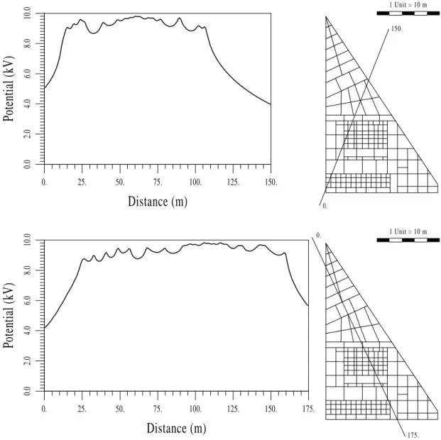
Results are given in table 2. Figure 2 shows the p otential distribution on
ground surface when a fault condition o ccurs, and p otential proles along
dierentlinesare represented ingure 3.
Numerical resolution of this mo del of the grounding grid has only required
seven and a half minutes of CPU time in a conventional p ersonal computer
(i.e.PC486/16Mb to 66MHz).
1
It is interesting tonotice that using one single constant leakage current density
element p er electro de, thenumb er ofdegrees of freedom in this example would b e
1 Unit = 10 m
3.0
4.0
5.0
6.0
7.0
8.0
9.0
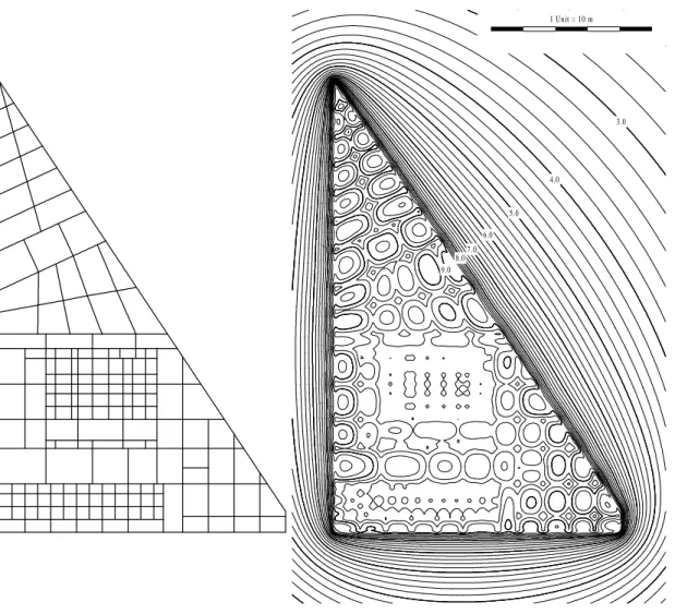
Fig.2.E.R.Barb eraGrounding Grid: Planand Potential Distributionon Ground
Surface (p otential contoursplottedevery 0.2kV,and thickcontoursevery 1 kV).
The secondexample that we present is the Balaidos I I substation grounding
op erated by the p ower company Union Fenosa, close to the city of Vigo in
Spain.The earthing systemof this substation isa grid of107 cylindrical
con-ductors(diameter:11.28 mm)buried toa depthof 80 cm,supplemented with
67 vertical ro ds (each one has a length of 2.5 mand adiameterof 14.0 mm).
The total surface protected up to 4800 m
2
. The total area studied is a
rect-angle of 121 m by 108 m, whichimplies asurface up to 13000 m
2
. As in the
previous case, the Ground Potential Rise considered in this study has b een
10 kV.Theplan of the groundinggrid andits characteristicsare presented in
gure 4and table 3.
The numericalmo delused inthe resolution ofthis problemisalsobased on a
Galerkin typ e weighting. Each bar is now discretizedin one single parab olic
free-0.
25.
50.
75.
100.
125.
150.
Distance (m)
0.0
2.0
4.0
6.0
8.0
10.0
Potential (kV)
1 Unit = 10 m
150.
0.
0.
25.
50.
75.
100.
125.
150.
175.
Distance (m)
0.0
2.0
4.0
6.0
8.0
10.0
Potential (kV)
1 Unit = 10 m
0.
175.
Fig. 3.E.R. Barb eraGrounding Grid: Potential prolesalong dierent lines.
dom 2
.
Results are given in table 4. Figure 4 shows the p otential distribution on
ground surface whena fault condition o ccurs.
Numericalresolutionofthis mo delhasonlyrequiredtenminutesofCPUtime
ina conventionalp ersonal computer(i.e. PC486/16Mb to 66MHz).
It can b e shown in this example that using parab olic elements increases the
totalnumb erof degreesoffreedom.Obviously,computationalcostdevotedto
matrix generation and linear solving is also increased, but the overall
com-2
In this case,the use of one single constant density element p er electro de would
imply a total of 174 degrees of freedom,while theuse of one single linear element
Balaidos I I Substation:Characteristics.
BALAIDOS I I GROUNDING SYSTEM
Max.GridDimensions: 60m280m
GridDepth: 0.80m
Numb er ofGrid Electro des: 107
Numb er ofVertical Ro ds: 67
Electro de Diameter: 11.28mm
Vertical Ro dDiameter: 14.00mm
GroundPotential Rise: 10kV
Earth Resistivity: 60m
1 Unit = 10 m
9.0
8.0
7.0
6.0
5.0
4.0
Fig. 4.Balaidos I I Grounding Grid: Plan (vertical ro dsmarked withblack p oints)
and Potential Distribution on Ground Surface (p otential contours plotted every
0.2kV,and thick contoursevery1 kV).
putingeort isacceptable (ofthe sameorder of magnitude)whileprecisionis
muchhigher.
Bothexampleshaveb eenrep eatedlysolvedincreasingthesegmentationofthe
electro des. At the scale of the whole grid, results and p otential distributions
on the earth surface were not noticeably improved by increasing
segmenta-tion. We conclude, as a general rule, that a reasonable (mo derate) level of
segmentationissucientfor practical purp oses.Increasing the numb erof
el-ements b eyond this p oint will not b e necessary unless high accuracy lo cal
Balaidos I I Substation:Numerical Mo del and BEMResults.
BALAIDOS I I GROUNDING SYSTEM:
1D BEM MODEL & RESULTS
Typ eof Element: Parab olic
Numb er ofElements: 174
Degrees ofFreedom: 315
Fault Current: 25kA
Equivalent Resistance: 0.4
CPU Time: 600s
Computer: PC486/16Mb/66MHz
nally,theuseofhigherorderelementswillb emoreadvantageous(ingeneral)
than increasing segmentation intensively, since accuracy will b e higher for a
remarkablysmallertotal numb erof degrees of freedom[8].
6 Conclusions
ABoundaryElementapproachfortheanalysisofsubstationearthingsystems
has b eenpresented. For 3D problems,some reasonable assumptions allow us
to reduce a general 2D BEM formulation to an approximated less exp ensive
1D version. By means of new advanced integration techniques, it is p ossible
tocomputeanalyticallyalltheco ecientsofthenumericalmo del,andreduce
computing requirementsin memorystorage and CPU timeunder acceptable
levels.
Severalwidespreadintuitivemetho ds canb eidentiedas theresultofsp ecic
choices for the test and trial functions and suitable assumptions intro duced
inthe BEMformulationto reducecomputationalcost. Problemsencountered
with the application of these metho ds can now b e nally explained from a
mathematicallyrigorous p oint of view,while moreecientand accurate
for-mulations can b e derived.
Nowadays, all these techniques derived by the authors have allowed to
de-velopa ComputerAidedDesign system(TOTBEM) [19]for earthing grids of
electrical substations. With this system, it is p ossible to analyze accurately
grounding gridsof medium/bigsizes,nearlyinreal timeand usinga lowcost
and widely available conventional computer.Obviously,the study of a larger
acceptable.
Acknowledgements
This work has b een partially supp orted by p ower company \Union Fenosa",
by research fellowships of the \Universidad de La Coru ~na " and the regional
government\Xunta de Galicia",and by aresearchproject of p owercompany
\Fecsa".
Appendix 1. The analytical expression for function 8(a;b) in (46) can b e
expressed as [8]
8(a;b)=V
(0) '
(0)
+V
(1) '
(1)
+V
(2) '
(2)
; (56)
where co ecients (V
(0)
;V
(1)
;V
(2)
) dep end on geometrical parameters of the
electro deand known values ofthe shap e function:
V (0)
= b n
0i +
b n 1i
b+
b n 2i
b 2
0a
2 =2
; V
(1) =
b n
1i
+2b
b n 2i
; V
(2) =
b n 2i
=2 ;
(57)
and functions '
(0)
;'
(1)
;'
(2) are
' (0)
=ArgSh
10b
a !
+ ArgSh
1+b
a !
(58)
' (1)
= q
(10b)
2
+a
2 0
q
(1+b)
2
+a
2
(59)
' (2)
=(10b)
q
(10b)
2
+a
2
+ (1+b)
q
(1+b)
2
+a
2
(60)
Appendix2. Derivationofanalyticalexpressionsforcomputingco ecients
in(55) requires aprevious geometricalanalysis of the relativep osition oftwo
arbitraryelements and in the3D space, so that allthe variablesinvolved
in c R
ji
( b
0 ;
b s ssssss sssssss
;L
;
b 0 ;
b s s s s s
ss
s s s s s s s
;L
) can b e expressed in terms of parameters that
dep endon the relativep osition b etweenthem.Thus,sinceweare considering
elements formed by rectilinear segments, we can take a co ordinates system
which origin is the mid-p oint of and the y-axis is placed on this segment.
Inthis co ordinates system,element can nowb e denedby anewmid-p oint
e 0
(
e 0x
; e 0y
; e 0z
) and a new axialunit vector
e s s s s s
ss
s s s s s s s
(e
s x ;
e s y ;
e s z
the geometricalinformationb etweenthe twosegmentsintermsof e 0 , e s s s s s ss s s s s s s s and lengthsL and L
. These quantitiesare
=
L
L
; A =
e 0y L =2 !
; B=
e s y (61) C 2 = e 0x L =2 ! 2 + e 0z L =2 ! 2 + 0 @ q ( =2) 2 +( =2) 2 L =2 1 A 2 (62) D= e 0x L =2 ! e s x + e 0z L =2 ! e s z ; E 2 =( e s x ) 2 +( e s z ) 2 (63)
Now, co ecientsK
(u) w
in (55) can b e computed,in termsof , A, B , C, D , E
and known values of shap e functions, as
0 B B B B B B B B B B B @ K (0) 0 K (0) 1 K (0) 2 K (0) 3 K (0) 4 1 C C C C C C C C C C C A = 0 B B B B B B B B B B @ b n 0j 0 0 b n 1j b n 0j 0 b n 2j b n 1j b n 0j 0 b n 2j b n 1j 0 0 b n 2j 1 C C C C C C C C C C A 0 B B B B B @ 1 A 2 (A 2 0C 2 =2) 0 B 2
(2AB0D)
0 0 2 (B 2 0E 2 =2) 1 C C C C C A 0 B B B B B @ b n 0i b n 1i b n 2i 1 C C C C C A (64) 0 B B B B B B B B B B B @ K (1) 0 K (1) 1 K (1) 2 K (1) 3 K (1) 4 1 C C C C C C C C C C C A = 0 B B B B B B B B B B @ b n 0j 0 b n 1j b n 0j b n 2j b n 1j 0 b n 2j 0 0 1 C C C C C C C C C C A 0 B B B @ 1 2A 0 2B 1 C C C A 0 B B B @ b n 1i b n 2i 1 C C C A ; 0 B B B B B B B B B B B @ K (2) 0 K (2) 1 K (2) 2 K (2) 3 K (2) 4 1 C C C C C C C C C C C A = 0 B B B B B B B B B B @ b n 0j b n 1j b n 2j 0 0 1 C C C C C C C C C C A 1 2 b n 2i (65)
On the other hand, computation of integral co ecients '
(u) w
in (55) can b e
summarizedin the followingexpressions:
b eing ' w
and '
w
' (0)A w
= Ifw g[a;b;c;d]
' (1)A w
= Jfw g[a;b;c;d]
with 8 > > > <
> > > :
a =
1
0A
b=0B
c 2
=C
2
+a
2
d=D0aB
(69)
' (0)B w
= Ifw g[a;b;c;d]
' (1)B w
= Jfw g[a;b;c;d]
with 8 > > > <
> > > :
a=0
1
+A
b=0B
c 2
=C
2
+a
2
d=D0aB
(70)
Ifmg[a;b;c;d]andJfmg[a;b;c;d]areintegralsthatcanb ecomputed
analyt-ically [8]for dierent orders 0 m 4. Resultant formulae willalso dep end
on parameters [a, b, c,d], which contain the informationab out the geometry
of the two elements and their relative p osition. The complete development
of these expressions and some discussions ab out their use can b e found in a
previous work [8].
Next,these analyticalformulae arepresented.In them,we haveused
geomet-rical parameters [a;b;c;d]and the following relationships:
R 2
=c
2
0d
2
; f =a0bd; !
2
=(c
2
0a
2
)(10b
2
)0(d0ab)
2
2
=R
2 b
2
+f
2
; r =
q
(d+1)
2
+R
2
; s=
q
(d01)
2
+R
2
(71)
Ifng=
j=n X
j=0
n
j
(0d) j
I 1
fn0jg (72)
I 1
fng =
(d+1)
n+1
n+1
ln(b(d+1)+r )0
(d01)
n+1
n+1
ln(b(d01)+s)
0 b
n+1
K 3
fn+1g; if b
2
=1 (73)
I 1
fng =
(d+1)
n+1
n+1
ln(a+b+r )0
(d01)
n+1
n+1
ln(a0b+s)
+ bf
n+1
K 1
fn+1g0
10b
2
n+1
K 1
fn+2g
0 bR
2
n+1
K 2
fn+1g+
f
n+1
K 2
Jfng = j=n X
j=0 n
j
(0d) j
J 1
fn0jg (75)
J 1
fng = K
3
fn+2g + R
2 K
3
fng (76)
K 1
fng =
1
10b
2 "
(d+1)
n01
0 (d01)
n01
n01
+2bfK
1
fn01g0(R
2
0f
2
)K
1
fn02g
#
(77)
K 1
f1g=
1
2(10b
2 )
"
ln r
2
0(a+b)
2
s 2
0(a0b)
2 !
+2bfK
1 f0g
#
(78)
K 1
f0g=
1
!
arctan 2!
c 2
0a
2
(79)
K 3
fng =
(d+1)
n01
n
r0
(d01)
n01
n
s0
(n01)R
2
n
K 3
fn02g (80)
K 3
f1g=r0s (81)
K 3
f0g=ArgSh
d+1
R !
0ArgSh
d01
R !
(82)
K 2
fng =
1
10b
2 "
K 3
fn02g+2fbK
2
fn01g0(R
2
0f
2 )K
2
fn02g
#
(83)
K 2
f1g=
1
s 0
1
r
; if b=f =0 (84)
K 2
f0g=
1
R 2
"
d+1
r 0
d01
s #
; if b=f =0 (85)
K 2
f1g=
f
2
"
ArgTh
a0b
s !
0ArgTh
a+b
r !#
+ R
2 b
! 2
"
arctan
!(a0b+bs)
! 2
+(d010ab+b
2
)(d01+s)
0arctan
!(a+b+br )
! 2
+(d+10ab0b
2
)( d+1+r )
#
(86)
K 2
f0g=
b
2
"
ArgTh
a+b
r !
0ArgTh
a0b
s
+ f
! 2
arctan
!(a0b+bs)
! 2
+(d010ab+b
2
)(d01+s)
0arctan
!(a+b+br )
! 2
+(d+10ab0b
2
)( d+1+r )
#
(87)
References
[1]ANSI/IEEEStd.80,IEEE Guide for safetyin ACsubstationgrounding (IEEE
Publ.,New York,1986).
[2]J.G. Sverak, W.K. Dick, T.H. Do dds and R.H. Hepp e, Safe substation
grounding(PartI),IEEETrans.onPowerApparatusand Systems 100(1981)
4281-4290.
[3]R.J. Hepp e, Computation of p otential at surface ab ove an energized grid or
otherelectro de, allowing fornon-uniformcurrent distribution, IEEETrans.on
Power Apparatus and Systems 98(1979)1978-1988.
[4]D.L.GarrettandJ.G.Pruitt,ProblemsencounteredwiththeAveragePotential
Metho d of analyzing substation grounding systems, IEEE Trans. on Power
Apparatus andSystems 104(1985) 3586-3596.
[5]E.Durand,
Electrostatique (Masson,Paris,1966).
[6]Ll. Moreno, Disseny assistit per ordinador de postes a terra en instal1lacions
electriques (Tesina de Esp ecialidad ETSECCPB, Universitat Politecnica de
Catalunya,Barcelona, 1989).
[7]F. Navarrina, I. Colominas and M. Casteleiro, Analytical integration
techniques for earthing grid computation by b oundary element metho ds.
Numerical Methods in Engineering and Applied Sciencies, Section VI I:
\Electromagnetics",1197{1206(H.Alder,J.C.Heinrich,S.Lavanchy,E.O ~nate,
B.Suarez(Editors);CentroInternacionaldeMeto dosNumericosenIngenier a,
CIMNE,Barcelona, 1992).
[8]I. Colominas, Calculo y Dise ~no por Ordenador de Tomas de Tierra en
Instalaciones Electricas: Una Formulacion Numerica basada en el Metodo
Integral de Elementos de Contorno (Ph.D. Thesis, E.T.S. de Ingenieros de
Caminos,Canales yPuertos,Universidadde La Coru ~na,La Coru ~na,1995).
[9]E.D.Sunde,Earth conduction eectsin transmissionsystems (McMillan,New
York,1968).
[10]R. Dautray, J.L. Lions, Analyse mathematique et calcul numerique pour les
scienceset les techniques,vol. 6 (Masson,Paris,1988).
[11]M. Kurtovic, S. Vujevic, Potential of earthing grid in heterogeneous soil,
International Journal for Numerical Methods in Engineering 31 (1991)
1979).
[13]O.D.Kellog,Foundationsof potentialtheory, (SpringerVerlag, Berln, 1967).
[14]I. Colominas, F. Navarrina and M. Casteleiro, A validation of the b oundary
elementmetho dforgroundinggriddesignandcomputation.NumericalMethods
in Engineeringand Applied Sciencies,Section VI I: \Electromagnetics", 1187{
1196 (H. Alder, J.C. Heinrich, S. Lavanchy, E. O ~nate, B. Suarez (Editors);
CentroInternacionaldeMeto dosNumericosen Ingeniera, CIMNE,Barcelona,
1992).
[15]C. Johnson, Numerical solution of partial dierential equations by the nite
element method (Cambridge Univ.Press, Cambridge, USA,1987).
[16]T.J.R.Hughes, Theniteelement method (PrenticeHall, New Jersey,1987).
[17]I. Colominas, F. Navarrina and M. Casteleiro, Formulas analticas de
integracion para el calculo de tomas de tierra mediante el meto do de los
elementos de contorno. Metodos Numericos en Ingeniera, Section: \Meto dos
Numericos",855{864(F.Navarrina,M.Casteleiro(Editors);So ciedadEspa ~nola
de Meto dosNumericos en Ingeniera SEMNI,Barcelona, 1993).
[18]G.Pini andG.Gamb olati,Is asimple diagonalscalingtheb estpreconditioner
forconjugategradientsonsup ercomputers ?,AdvancesonWater Resources 13
(1990)147-153.
[19]M. Casteleiro, L.A. Hernandez, I. Colominas and F. Navarrina, Memoria y
Manual deUsuario del SistemaTOTBEMpara Calculo y Dise ~noAsistido por
OrdenadordeTomasdeTierradeInstalacionesElectricas(E.T.S.deIngenieros
deCaminos,Canales yPuertos,Universidadde La Coru ~na,La Coru ~na,1994).
[20]I. Colominas, J. Aneiros, F. Navarrina and M. Casteleiro, A Boundary
Element Numerical Approach for Substation Grounding in a Two Layer
Earth Structure. Advances in Computational Engineering Science, Section:
\Recent Developments in Boundary Element Metho ds", 756{761(S.N.Atluri,