Essays on uncertainty, monetary policy and financial stability

(1)

Essays on Uncertainty, Monetary Policy

and Financial Stability

Alain Schlaepfer

TESI DOCTORAL UPF / ANY 2016

DIRECTOR DE LA TESI

Professor Jordi Gal´ı

(2)

(3)

Acknowledgments

I would like to thank my advisor Jordi Gal´ı. I have learned an immense amount from him during these years, and I am very thankful for all the ad-vice and support I received from him.

I thank Andrea Caggese and Vasco Carvalho for their help and support. Dur-ing my PhD studies, I benefited immensely from research stays at PUC Rio, BU and Stanford. I thank Carlos Viana de Carvalho, Simon Gilchrist and Ken Scheve for making them possible. I thank the SNF for financing my stay at BU. I am grateful for advice and feedback that I have received at various stages of my research, in particular from Alberto Martin, Xavier Freixas, Ander Perez, Fabio Canova and all participants of the CREi Macroeconomic Breakfast and International Lunch seminars.

Thanks to everybody that makes the functioning of UPF, CREi and BGSE possible, in particular Marta Araque, Laura Agust´ı, Carolina Rojas and Es-ther Xifre. I was always able to rely on your fantastic help in various situa-tions. Thank you to all my fellow PhD students at UPF, in particular Bruno, Tanya, Oriol, Gene, Jagdish, Tom, Marc, Miguel, Pietro and Alvaro. Thank you to Taulat 7A and my flatmates there, Pau for some days and Esteban for some years.

A special thanks to Eugenia Vella and Toni Rodon, who made the deposit of this thesis possible.

A big thank you to my brother Daniel and my sisters Sonja and Isabelle. I have often missed you guys during these years. Also to my father Rodolphe and my mother Marianne, for always having supported my along this jour-ney. Thank you Michael for being such a great friend.

Above all, I want to thank Vicky – not just for all the discussion, feedback, ideas, advice and general support, but most of all for making all these years fun and interesting.

(4)

(5)

Abstract

In the first chapter, I examine both theoretically and empirically how income uncertainty affects the effectiveness of monetary policy. I consider income risk from potential unemployment, and find that monetary policy has a smaller influence on aggregate demand when unemployment risk is high. I build on the fact that saving arising from a precautionary motive has a smaller interest elasticity. As a consequence, aggregate demand reacts less to the interest rate when uncertainty is high. The second chapter links the build-up of financial risk that led to the recent financial crisis to the preceding period of exceptionally low macroeconomic volatility. The degree of stability that a country has enjoyed before 2007 predicts robustly how much it suffered from the crisis, a result that also holds for individual firms. In the final chapter, I connect this period of low volatility to the conduct of monetary policy. Building on a stylized model, I show empirically that monetary policy may have been ‘too successful’ in stabilizing inflation, as this has contributed to excessive financial risk taking.

Resum

(6)

(7)

Preface

This dissertation has in many ways been influenced by the economic environ-ment during which it was written. I started my research at Pompeu Fabra in the aftermath of the Great Recession, the deep global economic downturn that followed the financial crisis of 2007-08. Soon after, a debt crisis took hold of Europe, which until now, while I am finishing my thesis, is far from being resolved. Many things that have happened were almost unimaginable as little as ten year ago: the financial sector as we know it would have been wiped out if it was not for an unprecedented intervention by central gov-ernments across the globe, several member countries of the European Union found themselves at the brink of defaulting and leaving the common cur-rency, experiencing deep slumps in output and unemployment rate surges of up to 30%. This profound economic disturbances came after a period of rel-ative calm and optimism. The new millennium started with the widespread believe that the problem of large economic fluctuations had essentially been solved, that central banks could focus on the task of ‘fine tuning’, and that the European unification and the introduction of the Euro would lead to prolonged growth and to convergence of standards of living across members countries. This relative calm was swept away, with economies around the globe experiencing large increases in uncertainty, and central banks under-taking unconventional policy measures in huge scales, while still struggling to prevent economic collapse. Intrigued by these events, I made uncertainty the central focus of my dissertation research. Much of this dissertation deals with how uncertainty affects the behavior of individuals and of firms, and how, as a consequence, it changes the impact of policy measures on macroe-conomic outcomes.

(8)

if unemployment risk is high, households engage in precautionary saving to protect themselves against potential income shocks. Second, saving that is done for a precautionary motive responds little to changes in the interest rate,i.e. the interest elasticity of precautionary saving is near zero. Thirdly, a low interest elasticity of saving, and hence also of demand, implies that conventional monetary policy struggles in stimulating the economy through changes in the real rate. To illustrate this mechanism, I construct a styl-ized New Keynesian model with heterogeneous households, which allows for comparing responses to monetary policy shocks across economies with dif-ferent unemployment risk. My empirical results support the finding that income risk from unemployment limits the effectiveness of monetary policy. Using household level data from the US, I find that consumption responses to changes in the real rate are smalll for households that have a high risk of becoming unemployed, and for households that live in states with low unem-ployment insurance benefits. These results also hold on an aggregate level: both within US states and within Euro Area countries, I find that regions with high unemployment or low insurance benefits are less affected by mon-etary policy.

(9)

(10)

(11)

Chapter 1 UNEMPLOYMENT RISK,

PRECAUTIONARY

SAVINGS, AND THE

EFFECTS OF MONETARY

POLICY

1.1 Introduction

(14)

A change in the interest rate has two opposing effects on household consump-tion and saving rates. Consider a reducconsump-tion in the real interest rate. The substitution effect, due to changes in intertemporal prices of consumption, gives households incentives to reduce savings and increase current consump-tion. On the other hand, a lower interest rate reduces the future value of savings, a negative wealth effect to which households react by cutting cur-rent spending. In a standard New Keynesian model, the substitution effect dominates, implying a negative interest elasticity of savings. But the pres-ence of precautionary savings alters this picture. Large uncertainty about future income means that there may exist low income states in which a po-tentially lower consumption level is mainly financed out of savings, implying high marginal utilities derived out of savings. Consequently, the wealth ef-fect of a reduction in the real interest rate is larger than the substitution effect, driving the interest elasticity of savings towards zero or even turning it negative. In such a situation, a central bank policy which lowers interest rates in order to stimulate demand will not be successful.

(15)

I then proceed to provide empirical support for the suggested relationship between unemployment risk and the effectiveness of monetary policy. Using the US Consumption Expenditure Survey, I document that consumption re-acts less to changes in the interest rate if the household faces a high risk of losing a job, or if it resides in a state with low unemployment benefits. I then use aggregate data from US states and Euro area countries and show that the negative association between the real interest rates and economic perfor-mance goes towards zero in regions with higher unemployment rates as well as in regions with lower unemployment benefits, as measured by replacement rates. Taken together, the data provides strong support for the the notion that unemployment risk dampens the response to monetary policy shocks.

(16)

of the feedback loop between unemployment risk and precautionary savings during the Great Recession is documented in Challe et al. (2015). Finally, and probably most similar in spirit to this paper, Paoli and Zabczyk (2013) focus on cyclical fluctuations of precautionary savings, showing that policy responses need to be stronger when accounting for an increase in uncertainty during a downturn.

The relevance of precautionary savings is empirically well documented (see e.g Carroll (1994), Cagetti (2003), Lusardi (1998), Carroll et al. (2012)). Gourinchas and Parker (2001) point out the importance of precautionary savings with respect to aggregate fluctuations. Similar to this paper, Engen and Gruber (2001) use differences in unemployment insurance replacement rates across US states to identify a motive for precautionary saving. Simi-larly, there is a large body of literature, starting with the seminal paper of Hall (1978), aiming at estimating interest elasticities. Gruber (2013) pro-vides an excellent review. Contributions that link the level of precautionary savings to interest elasticities include Carroll (1992), who notes that interest rates have little effect on wealth accumulation, if the latter is a buffer stock against negative shocks. Bernheim (2002) concludes that the interest elastic-ity of savings can fall considerably after accounting for precautionary savings, while Engen and Gale (1997) find that savings are relatively insensitive to the rate of return if done for precautionary reasons. Cagetti (2001) confirms these findings of a low interest elasticity in the presence of precautionary savings.

(17)

house-holds from income shocks, in particular unemployment and other forms of social insurance, as well as potentially public employment programs, can help to avoid reaching such a state. And finally, an increase in inequality, as long as it goes in hand with increases in individual income fluctuations, can re-duce the effectiveness of monetary policy.

The remainder of this paper is structured as follows. Section 1.2 provides a theoretical discussion of how uncertainty affects the interest elasticity of sav-ing. The baseline New Keynesian model with unemployment risk is presented in section 1.3. Section 1.4 describes the calibration and solution method, as well as results and predictions from model simulations. Section 1.5 discusses extensions of the model, and shows that predictions continue to hold after accounting for endogenous government debt and the effects of monetary pol-icy on unemployment risk. Section 1.6 provides empirical support for the theory, and finally, section 1.7 concludes.

1.2 Precautionary saving and interest

elastic-ity

In this section, I investigate theoretically how the interest elasticity of savings depends on uncertainty. I show that under relatively general assumptions, the interest elasticity is smaller if savings arise from a precautionary motive. I analyze the saving decision in a two-period endowment economy with addi-tively separable utilityU =u(c1) +βE{u(c2)}, whereuis twice differentiable

and strictly concave. The utility function is assumed to exhibit decreasing absolute prudence, so that c > c > c implies

−u

00₍_c₎₋_u00₍_c₎

u0₍_c₎₋_u0₍_c₎ >−

u00(c)−u00(c)

u0₍_c₎₋_u0₍_c₎

(18)

Relative Risk Aversion function. For a good discussion of why decreasing absolute prudence is a natural condition to require of utility functions, see Kimball (1990).

Consider two individuals,x and y, who face budget constraints of the form

ci₁ =I−bi ci₂ =I₂i +Rbi

for i ∈ {x, y}. Note that income in the first period is the same for both individuals. Second period income of individual x is given by I₂x = I −φ, 0< φ <1, whileI₂y =I−ξwith probabilitypandI₂y =I+ξwith probability 1−p, 0< ξ <1. Optimal saving is given by the first order condition

1 = βRE

(

u0 ci₂∗ u0 _ci

1

∗

)

(1.1)

We focus on the case where ξ(φ) is defined such that for given parameter values, bx∗ = by∗. Note that then the two individuals are observationally equivalent in the first period, as they have identical income, consumption and saving. But the motive for saving varies: individual x saves because of a certain reduction of income in period 2. Expected income is the same in period 2 as in period 1 for individual y, but uncertainty about period 2 income gives rise to a precautionary motive. Individualysaves because there is a possibility of a large reduction in future income. The intuition for why this matters for interest elasticities can be gained from (1.1). Consider an increase in the interest rateR. As a direct effect, the RHS goes up, requiring an upward adjustment in u0(c1) (and downward in u0(c2)),i.e. a decrease in

c1 (and increase inc2), which is achieved through an increase in saving. This

is the substitution effect. The indirect wealth effect works through the fact that with an higher interest rate, available resources in period 2 increase, so

c2 increases for a givenb, thusc1goes up andbgoes down, partially offsetting

the substitution effect. For a prudent individual, this channel is stronger at states where c2 is small and thus the slope of marginal utility particularly

(19)

loss in future income, reducing the interest elasticity of saving.

To formally derive this result, I first state the interest elasticity as

∂bi∗

∂R

R bi∗

=−β[E{u

0 _ci

2

∗

}+RbE{u00 ci₂∗}]

β∗R2_E_{_u00 _ci

2

∗

}+u00₍_c

1)

R bi∗

= A+C E{u

00 _ci

2

∗

}

B−C E{u00 _ci

2

∗

}

where I made use of the first order condition (1.1) and defined A = u0(c1),

B = −bu00(c1), and C = βR2b. A, B and C are all strictly positive and

constant across individuals. Thus, the last expression is strictly increasing inE{u00 ci

2

∗

}, and to show that a precautionary saving motive reduces the interest elasticity, it is sufficient to show that u00(cx

2

∗₎_{> E}_{_u00 _cy

2

∗

}.

Condition (1.1) together with cx

1

∗ ₌ _cy

1

∗

implies that u0(cx

2

∗_{) =} _pu0 _c

2y∗

+ (1−p)u0(c2y∗), where c2y∗ = I − ξ +Rb∗ and c2y∗ = I +ξ +Rb∗, with

c2y∗ > cx2

∗

> c2y∗. Using decreasing absolute prudence we can write

u0(cx₂∗) =pu0 c2y∗

+ (1−p)u0(c2y∗)

pu

0₍_cx

2

∗₎₋_u0 _c

2y∗

u0₍_c

2y∗)−u0(cx2∗)

= (1−p)

pu

00₍_cx

2

∗₎₋_u00 _c

2y∗

u00₍_c

2y∗)−u00(cx2

∗₎ >(1−p)

u00(cx₂∗)> pu00 c2y∗

+ (1−p)u00(c2y∗)

u00(cx₂∗)> Eu00 cy₂∗

which proves that the interest elasticity of saving that arises from a precau-tionary motive is indeed smaller.

(20)

cur-rent interest rate. Figure 1.1 shows saving for diffecur-rent levels of the interest rate. The solid blue line represents individualx, characterized by a lower but certain second period income, while the dashed green line represents the in-dividual with uncertain income. Saving behavior is significantly less sensitive to changes in the interest rate if the saving motive results from uncertainty over future income. In fact, atR = 1/β, the interest elasticity of individual

[image:20.595.148.466.349.592.2]

x is equal to 1, while equaling only 0.67 for individual y.

Figure 1.1. Savings of individual with certain future income (solid blue line) and uncertain income (dashed green line)

1.3 A New Keynesian model with

precaution-ary saving

(21)

are kept as simple as possible, in order to highlight the suggested relation-ship between unemployment risk and the effects of monetary policy. As in the standard model, nominal rigidities allow firms to only readjust their prices periodically, giving rise to monetary non-neutrality. Agents are het-erogeneous with respect to their labor market status. Employed households face an exogenous probability of losing their job each period. Unemployed households do not work and hence receive no labor income, but a (smaller) payment from unemployment benefits. This risk of a future state with lower income gives employed agents an incentive to accumulate precautionary sav-ings. In line with the goal to keep the model simple, there is no capital in this economy. Instead, agents save using government bonds.

1.3.1 Households

The economy has a population of size one. A share νt of households are

employed, and face the risk of getting unemployed the next period with probability ρt+1. The unemployed, constituting a share of 1−νt of the

pop-ulation, receive unemployment benefits of real value s from the government, which together with past savings are used to finance consumption. Agents are credit constrained, as financial wealth is restricted to be non-negative. An employed household uses income from work and savings to consume and to buy government bonds. The government taxes employed workers lump-sum to finance unemployment benefits and bond returns.

An employed household’s budget constraint is thus given by

Z

Pt(i)ct(i)di+bt=wtht+ (1 +it−1)bt−1 −Tt+Dt (1.2)

whereitis the nominal interest rate,htdenotes hours worked,wtis the hourly

wage rate and Dt are dividend payments. Households maximize expected

lifetime utility of the form

∞

X

t=0

βtE0

ct1−σ −1

1−σ −ψ h1+_t ϕ

1 +ϕ

exp(xt)

(22)

subject to (1.2), where ct is a consumption index given by

ct≡

Z 1

0

ct(i)1−

1

di.

−1

The preference shifter xt is assumed to follow an AR(1) with mean zero and

lag-term coefficient ρx ∈[0,1). As usual, demand for variety iis given by

ct(i) =

Pt(i)

Pt

−

where the price index is defined as Pt≡

R1

0 Pt(i)

1−_di.

1 1−

.

The first order conditions can then be written as

wt

Pt

=ψctσhϕt (1.4)

1 =β(1 +it)Et

ct

ct+1

σ

1 Πt+1

exp(xt+1−xt)

(1.5)

Denoting consumption of an employed and an unemployed household with

ce _and _cu_{, respectively, (1.5) becomes}

1 =β(1+it)Et

ρt+1

ce t cu t+1 σ

+ (1−ρt+1)

ce t ce t+1 σ 1 Πt+1

exp(xt+1−xt)

(1.6) Unemployed households do not work and consume all available income. Thus we have

cu_t = (1 +it−1)bt−1/Pt+s (1.7)

To keep the model tractable, it is assumed that once a household gets un-employed, it lives for one more period and then dies, ensuring that all avail-able resources are consumed in the last period. The household gets replaced with a newborn, which is employed with probabilityζt and unemployed with

probability 1− ζt. A newborn household receives an initial transfer from

(23)

wealth dispersion within household types, and thus considerably simplifies the model. ζt is determined by the separation rate ρt and employment rate

νt.

1.3.2 Firms

Firms use labor as the only input to produce a differentiated good indexed by i ∈ [0,1]. Technology is identical across firms and represented by the production function

Yt(i) = At(hdt(i))

1−α

(1.8) where at ≡ log(At) follows an AR(1) process with mean zero and lag-term

coefficient ρa ∈ [0,1). Price stickiness is modeled following Calvo (1983),

assuming that only a fractionθ of firms can adjust prices in any period.

The firm side is identical to Gal´ı (2015), where a careful derivation can be found. It is shown that the production structure leads to an inflation equation of the form

πt =βEt{πt+1} −λ(µt−µ) (1.9)

whereπt is the log of gross inflation, µ=log(₋₁) is the desired log mark-up

over marginal costs and λ = (1−θ_θ)(1₍₁₋−_αβθ₊_α)(1₎−α). The average log mark-up is approximated with

µt=log(

Pt(1−α)At

wt(hdt)α

) (1.10)

1.3.3 Monetary and fiscal policy

The central bank sets the nominal interest rate following a Taylor-type rule of the form

(1 +it) =

1

r

Πt

Π

φ

exp(ut) (1.11)

where the monetary policy shock ut follows an AR(1) process with mean

zero and lag-term coefficient ρu ∈ [0,1). The target gross inflation rate of

(24)

The government issues bonds and collects taxes from employed workers to finance unemployment benefit transfers and for the repayment of maturing bonds. It is assumed that the government issues a constant real quantity of one-period bonds, i.e. bt/Pt = b. Taxes are collected lump-sum from

em-ployed households and are adjusted to balance the budget period-by-period, so that

Tt=

1

νt

(1 +it−1)

Πt

−1

b+ (1−νt)s

1.3.4 Equilibrium

After imposing the market clearing conditions for the markets for goods and labor, given by

Yt(i) = νtcet(i) + (1−νt)cut(i)

hd_t =νtht

the equilibrium dynamics are defined by combining the labor supply (1.4), the Euler equation for employed households (1.6) and unemployed consump-tion (1.7), with the producconsump-tion funcconsump-tion (1.8) and the equaconsump-tions determining marginal costs (1.10) and inflation dynamics (1.9), as well as the monetary policy rule (1.11) and three processes for the exogenous shocks.

1.4 Calibration and Results

(25)

rule to approximate integrals in the expectation terms. I then use the Euler equation (1.6) and inflation dynamics (1.9) to update the guess. Iterating on this step until the guesses converge then yields the solution for the policy functions, from which both the risky steady state and the full dynamics of the model can be computed.

To illustrate the suggested mechanism, the model is first solved for three different economies that are identical except for differences in the separation rate (and corresponding differences in the labor market status of newborns), which itself remains constant over time. The employment parameter ν is fixed at 0.92, corresponding to an unemployment rate of 8%. The economies studied differ only in their separation rates, which are 1%, 4% and 7%, respec-tively.1 _{While the assumption of an unemployment rate that is independent}

of the separation rate is unrealistic, it is very useful as a first exercise for il-lustrative purposes. Unemployed consumption is by assumption independent of future interest rates, hence the elasticity of aggregate consumption with respect to the interest rate depends on the size of the pool of unemployed workers. To control for this channel, the unemployment rate is set to a con-stant value across economies. All remaining differences are then due to the precautionary saving motive of employed workers, induced by the separation rates. In the next section, I will consider the case were both the separation rate and unemployment react endogenously to labor market conditions.

All parameter values are reported in Table 1.1. The remaining values are standard in the literature and are not crucial for the qualitative results of the exercise. The central bank is assumed to follow an annualized inflation target of 2%, while the coefficient on inflation in the Taylor rule is set at 2. Fiscal policy is chosen such that in the steady state, the ratio of debt to annualized GDP equals 0.5.

(26)

[image:26.595.186.451.149.349.2]

Table 1.1. Parameter values

Parameter Value Parameter Value

β 0.99 Π 1.005

σ 1.5 φ 1.5

ϕ 1

ψ 1 b/yss 2

6

ρa 0.95

α 0.33 σa 1

θ 0.75 ρu 0.5

σu 1

ν 0.92 ρx 0.5

ρ 0.01, 0.04, 0.07 σx 1

s 0

(27)

[image:27.595.128.420.180.421.2]

Figure 1.2. Steady state values for economies with ρ = 0.04 (blue) and

ρ= 0.07 (red), in percentage difference to benchmark economy withρ= 0.01.

While the interest rates vary wildly across economies, differences are close to zero for all other steady state values. Hours are slightly lower if the sepa-ration rate is high, amounting to a decrease of steady state output of 0.09% if ρ= 0.04 and of 0.18% ifρ= 0.07. In accordance with the lower hours and decreasing returns, real wages are higher, but also this difference is very small.

(28)

[image:28.595.162.480.174.347.2]

Figure 1.3. Impulse responses to contractionary monetary policy shock, sep-aration rates set atρ= 0.01 (blue), ρ= 0.04 (green), and ρ= 0.07 (red).

Figure 1.4. Impulse responses to expansionary monetary policy shock, sepa-ration rates set atρ= 0.01 (blue), ρ= 0.04 (green), and ρ= 0.07 (red).

[image:28.595.164.482.450.622.2]

(29)

in the economy with the lowest unemployment risk, while output drops of 1.16% and 0.92% are observed in the other two cases. Economies with a higher separation rate also experience a smaller reduction in consumption of employed households, hours and inflation. Equivalent differences emerge when looking at an expansionary shock. The key to understanding the mech-anism lies in observing the reaction of consumption of the unemployed. Con-sider an expansionary monetary policy shock. This is reflected in a drop in the nominal rate and and an accompanying increase in the inflation rate, both leading to a decline in the real interest rate. With returns to savings going down, the consumption of unemployed households has to go down as well, since they finance consumption out of savings. As shown in the figures, unemployed consumption drops by a similar amount in all three economies. This in turn directly strengthens the precautionary saving motive of employed households, particularly so in economies with a high transition probability to unemployment,i.e. a large ρ. In consequence, we observe a smaller increase in employed consumption and hence in employment when the separation rate is higher.

Finally, note that the smallest response in the interest rate is observed in the economy with low unemployment risk. This is simply due to the endoge-nous reaction of the central bank to the drop in inflation, as implied by the assumed Taylor rule. Nevertheless, this reaction is not sufficient to offset the effects of the precautionary saving motive. In conclusion, the model predicts a stronger effect of monetary policy in economies with low unemployment risk.

1.5 Model extensions

(30)

issued is constant across economies (while the interest rates are allowed to vary). Instead, I assume that fiscal policy targets a steady state nominal rate that is equal in all economies, and adjusts debt issuance accordingly. In the previous exercise, a precautionary saving motive was reflected in lower real rates, while actual levels of savings were exogenously given. Now, savings lev-els are allowed to vary across economies. In all economies, it is assumed that the government targets a gross nominal rate of 1.02%. As a second change, economies will no longer differ with respect to their separation rates, which is now set at 4% for all economies. Instead, the generosity of unemployment insurance benefits will determine variations in income risk across economies. In particular, it is assumed that unemployment benefits s are equal to 0.05, 0.15, and 0.25, respectively, where higher values imply a lower income risk due to unemployment and hence a less strong precautionary savings motive.

Steady states values are again very similar across economies, with the ex-ceptions of debt levels, where large differences prevail. Compared to the low risk benchmark economy with s = 0.25, steady state levels of government debt are 71% and 143% higher in the economies with lower unemployment insurance parameters of 0.15 and 0.05, respectively. Looking again at impulse responses to a monetary shock reveals that also under the new assumptions, the suggested relationship between unemployment risk and monetary policy effects still holds2_{. Responses to a contractionary and an expansionary}

mon-etary shock, each of one standard deviation size, are shown in Figures 1.5 and 1.6, respectively.

2_{It is important to point out that there is no necessity for the two changes in}

(31)

[image:31.595.122.439.187.359.2]

Figure 1.5. Impulse responses to contractionary monetary policy shock, un-employment benefits set at s = 0.25 (blue), s = 0.15 (green), and s = 0.05 (red).

Figure 1.6. Impulse responses to expansionary monetary policy shock, un-employment benefits set at s = 0.25 (blue), s = 0.15 (green), and s = 0.05 (red).

[image:31.595.126.438.470.643.2]

(32)

pre-cautionary saving motive in the economy. If unemployment protection is high and income risk relatively small, this motive is weak and we see a large reaction of output. In the economy with s = 0.25, on impact output is reduced by 0.84% after a contractionary shock. When unemployment insur-ance benefits are decreased tos = 0.15 ands = 0.05, this response is reduced to 0.65% and 0.48%, respectively. An equivalent picture emerges after an ex-pansionary shock: a central bank is more successful in stimulating demand if unemployment protection is relatively strong.

Unemployment so far was treated as exogenous and constant, but it is im-portant to consider that monetary policy itself affects unemployment risk and hence the precautionary savings motive. To do so, the original model is extended with employment and separation rates that react endogenously to labor demand. To keep things simple, I postulate a proportional relationship between employment and labor demand of the form

νt=ν

ht

h

χ

where ν is chosen so that steady state employment is again at 0.92 as in the previous section, and χ is set at 0.5. The latter implies that half of the changes in total hours occur through adjustments at the extensive margin.

I further assume that separation rates move one to one with unemploy-ment by specifying

ρt =ρ

1−νt

1−ν

where ρ corresponds to the steady state value of ρt. All other parameter

(33)

strength-ened, particularly in economies with high separation rates. We again see that countries with high unemployment risk react less to a monetary impulse.

(34)

Figure 1.7. Impulse responses to contractionary monetary policy shock, un-employment benefits set at ρ = 0.01 (blue), ρ = 0.04 (green), and ρ = 0.07 (red).

(35)

1.6 Empirical analysis

This section turns to an empirical investigation of the suggested link between effectiveness of monetary policy and unemployment risk. The theory in the previous chapter predicts that with increasing unemployment risk, either through higher transition rates into unemployment or lower benefits, there is a smaller effect of changes in the interest rate on economic activity, due to a reduced response of households. I present support for these predictions in two steps. First, using household level data on consumption expenditure, section 1.6.1 shows that households’ consumption reacts more strongly to changes in the interest rate if unemployment risk is low. In section 1.6.2, I show that this carries over to the macro level, by examining the performance of US states in response to the federal funds rate, and the effect of the ECB policy rate on activity in Euro area countries. All these cases have the advantage that monetary policy is (approximately) independent of idiosyncratic household or regional shocks, which allows for relating differences in regional responses to interest rate changes with differences in their region specific characteristics. This strategy is particularly promising, since we are not interested in the average response to an interest rate change, but in how this response differs depending on unemployment risk.

1.6.1 Consumption expenditure at the household level

(36)

I do not consider the average effect of the interest rate on consumption. In-stead, I look at how this effect differs across households and regions. If the stimulating effect of an interest rate reduction is lower when unemployment insurance benefits are smaller, we would expect the interaction coefficient of the interest rate with the loss of income in case of unemployment should to be positive. Similarly, we would expect a positive interaction coefficient between the job loss risk faced by a household and the interest rate.

To test the first prediction, I construct the average loss rate U I which is equal to one minus the average statewide unemployment benefit replacement rate, i.e. the average income loss in case of unemployment. I then estimate regression equations of the form

yi,c,t =c+β¯rt−1+γr¯t−1∗U Ic+ [δ1+δ2r¯t−1]∗Xi,c

+δ3r¯t−1∗Zc+mc+nt+i,c,t (1.12)

whereyi,c,t are log consumption expenditures of householdiin statecat time

t. Data is of quarterly frequency and spans 1996 to 2014, and the sample contains all households where at least one member is employed at the time of the interview. As described above, ¯rt−1 is the four quarter average of the

real interest rate. The coefficient of interest is γ, which measures how the effect of the interest rate depends on unemployment risk. Xi,c and Zc are

household and state level controls, respectively. I interact this controls with the interest rate measure to capture their potential effect on the elasticity of consumption. At the households level, these controls include various socio-economic characteristics such the main earner’s education, occupation, race, gender, marital status, age and age squared, as well as the size of the house-hold. At the state level, additional controls on the size of the financial sector are included. Finally,mc and nt are state and period fixed effects.

(37)

[image:37.595.83.470.247.487.2]

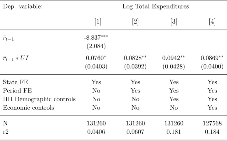
interest rate. As can be seen in column (1) the effect is relatively small, yet clearly not negligible: moving from the highest loss rate (0.54) to the lowest (0.31) increases the effect of interest rate changes on consumption by 1.75%. The coefficient is remarkably constant across specification with additional controls.

Table 1.2. Unemployment insurance

Dep. variable: Log Total Expenditures

[1] [2] [3] [4]

¯

rt−1 -8.837∗∗∗

(2.084) ¯

rt−1∗U I 0.0760∗ 0.0828∗∗ 0.0942∗∗ 0.0869∗∗

(0.0403) (0.0392) (0.0428) (0.0400)

State FE Yes Yes Yes Yes

Period FE No Yes Yes Yes

HH Demographic controls No No Yes Yes Economic controls No No No Yes

N 131260 131260 131260 127568 r2 0.0406 0.0607 0.181 0.184

Notes: Significance levels: *** p<0.01, ** p<0.05, * p<0.1. All regressions estimated by OLS. ¯ris the four quarter average of the federal funds rate, adjusted for inflation. U I

is one minus the state level average unemployment benefit replacement rate. Household demographic controls include the main earners age, age squared, race, gender, marital status, education level, occupation, as well as household size. Economic controls include the state level share of the financial sector. All regressions include interactions of the controls with the interest rate. Standard errors are clustered at the state level.

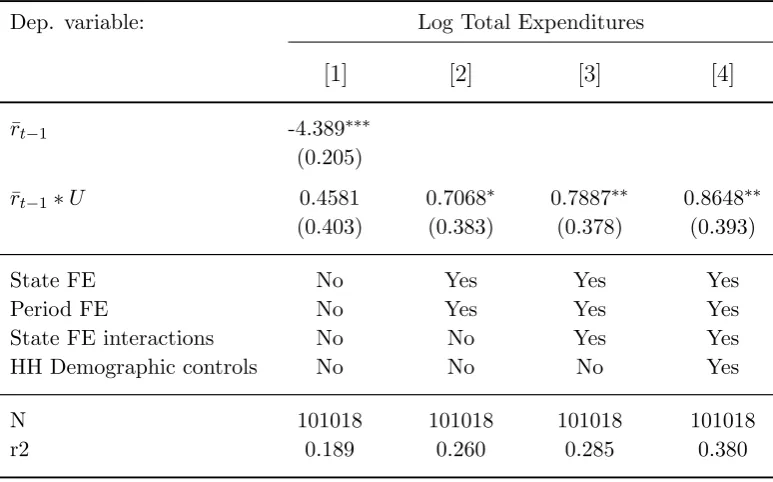
The risk of losing one’s job should similarly affect the reaction of con-sumption expenditures to the interest rate. To test for this, I construct a household level measure of job loss risk in the following four quarters.3 I estimate a model with transition to unemployment as dependent variable, using household level characteristics, including education and age of the main earner and the type of employment. This allows me to predict each employed

(38)

household’s risk of job loss in the following year. I use this measure of job loss risk interacted with the interest rate in regression equations equivalent to (1.12), where the income loss variable U Ic is now replaced with the job

loss risk Ui,c. The coefficient of interest is again γ, which is expected to be

positive. The fact that the risk of job loss is measured at the household level allows me to estimate within state effects of unemployment risk, by including in the specification state fixed effects interacted with the interest rate. Ta-ble 1.3 reports interaction coefficients of job loss risk with the interest rate. While insignificant in the specification without fixed effects, the estimates of γ are large and significant in all other models, indicating that a one per-centage point increase in the risk of job loss reduces the stimulating effect of an interest rate reduction by up to 0.86%. The effect increases in size with the addition of controls and gains significance at the 95% confidence level. Standard errors are bootstrapped to take into account that the regressor of interest is a predicted variable.

1.6.2 Evidence from US states and Euro zone countries

(39)

[image:39.595.83.470.151.392.2]

Table 1.3. Unemployment risk

Dep. variable: Log Total Expenditures

[1] [2] [3] [4]

¯

rt−1 -4.389∗∗∗

(0.205) ¯

rt−1∗U 0.4581 0.7068∗ 0.7887∗∗ 0.8648∗∗

(0.403) (0.383) (0.378) (0.393)

State FE No Yes Yes Yes

Period FE No Yes Yes Yes

State FE interactions No No Yes Yes HH Demographic controls No No No Yes

N 101018 101018 101018 101018 r2 0.189 0.260 0.285 0.380

Notes: Significance levels: *** p<0.01, ** p<0.05, * p<0.1. All regressions estimated by OLS. ¯r is the four quarter average of the federal funds rate, adjusted for inflation.

U is the predicted probability of household job loss within the next year. Household demographic controls include the main earners age, age squared, race, gender, marital status, education level, occupation, as well as household size. All regressions include interactions of the controls with the interest rate. Bootstrapped standard errors (for predicted regressors) in parenthesis.

I estimate equations of the form

yc,t=const+

2

X

τ=1

ατyc,t−τ +βr¯t−1+γr¯t−1∗Uc+δUc+c,t (1.13)

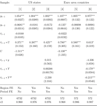
where the dependent variable yc,t is real income in the case of US states and

real GDP for Euro countries, both measured as their log deviation from the long run trend. The monetary policy term ¯r represents the four period aver-age of the real relevant interest rate, i.e. the federal funds rate and the main refinancing rate, respectively, adjusted for inflation. Uc is a region’s

(40)

which measures how the effect of monetary policy depends on the unemploy-ment rate. So failure of a decrease in the interest rate to stimulate economic activity implies γ > 0 (together with β < 0). In extended specifications, I add region and period fixed effects, as well as additional interactions of ¯rt−1.

The latter include interactions with initial level, per capita measures and growth rates of income or GDP. Controlling for these additional interaction terms strengthens the confidence thatγ is indeed capturing the effect of in-creased unemployment risk, and not additional channels such as the general economic situation in a region.

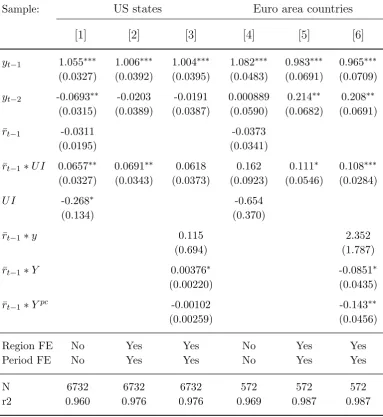
Table 1.4 reports results for US states (columns 1-3) and Euro area countries (columns 4-6). For US states, and as shown in column 1, the estimated coef-ficient β is negative, implying that an increase in the (four quarter average) federal funds rate of 100 basis points is followed by a reduction of real income by 0.94%, relative to trend income, for a state with a zero percent unemploy-ment rate. Note that these estimates do not have a causal interpretation, since interest rate changes should be correlated with expected mean income growth. Of more interest is the coefficientγ, which shows how the response of each state depends on unemployment risk. As suggested by the theory,γ

(41)

[image:41.595.87.471.152.571.2]

Table 1.4. Deviation from trend

Sample: US states Euro area countries

[1] [2] [3] [4] [5] [6]

yt−1 1.054∗∗∗ 1.004∗∗∗ 1.002∗∗∗ 1.107∗∗∗ 1.005∗∗∗ 0.977∗∗∗

(0.0327) (0.0389) (0.0392) (0.0687) (0.132) (0.122)

yt−2 -0.0681∗∗ -0.0181 -0.0172 -0.135∗ -0.00698 0.00981

(0.0314) (0.0385) (0.0384) (0.0644) (0.130) (0.122) ¯

rt−1 -0.0168 -0.0322

(0.0105) (0.0192) ¯

rt−1∗U 0.371∗∗ 0.387∗∗ 0.425∗∗ 0.780∗∗ 0.580∗∗∗ 0.613∗

(0.153) (0.160) (0.159) (0.305) (0.161) (0.319)

U -1.511∗∗ -3.130∗∗ (0.626) (1.235) ¯

rt−1∗y 0.315 -4.336

(0.563) (4.658) ¯

rt−1∗Y 0.00288 -0.179∗∗

(0.00178) (0.0584) ¯

rt−1∗Ypc -2.230 -0.215∗∗∗

(2.316) (0.0540)

Region FE No Yes Yes No Yes Yes Period FE No Yes Yes No Yes Yes

N 6732 6732 6732 572 572 572 r2 0.960 0.976 0.976 0.968 0.986 0.987

Notes: Significance levels: *** p<0.01, ** p<0.05, * p<0.1. All regressions estimated by OLS. The dependent variable is the deviation from trend of log real income of US states in columns (1)-(3), and of log real output of Euro area countries in columns (4)-(6). ¯r is the four quarter average of the federal funds rate, adjusted for inflation. U is the average regional level unemployment rate in the five years before sample start. y,Y, andYpcare average regional level output growth, log output and log output per capita, respectively, in the five years before sample start. Standard errors are clustered at the regional level.

(42)

percent increase in initial unemployment leads to a reduction in the effect of interest rates on output of 0.78 percentage points. Despite the smaller sample size, the estimated interaction coefficient is significant at the 95% confidence level, and relatively robust to the inclusion of country and period fixed effects, as well as of additional interaction terms. Confidence is reduced to 90% in the latter case, but the size of the coefficients remains large.

(43)

[image:43.595.86.471.152.571.2]

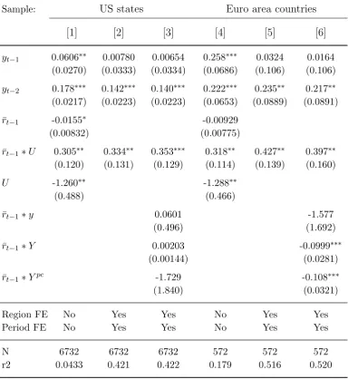
Table 1.5. Growth rates

[1] [2] [3] [4] [5] [6]

yt−1 0.0606∗∗ 0.00780 0.00654 0.258∗∗∗ 0.0324 0.0164

(0.0270) (0.0333) (0.0334) (0.0686) (0.106) (0.106)

yt−2 0.178∗∗∗ 0.142∗∗∗ 0.140∗∗∗ 0.222∗∗∗ 0.235∗∗ 0.217∗∗

(0.0217) (0.0223) (0.0223) (0.0653) (0.0889) (0.0891) ¯

rt−1 -0.0155∗ -0.00929

(0.00832) (0.00775) ¯

rt−1∗U 0.305∗∗ 0.334∗∗ 0.353∗∗∗ 0.318∗∗ 0.427∗∗ 0.397∗∗

(0.120) (0.131) (0.129) (0.114) (0.139) (0.160)

U -1.260∗∗ -1.288∗∗ (0.488) (0.466) ¯

rt−1∗y 0.0601 -1.577

(0.496) (1.692) ¯

rt−1∗Y 0.00203 -0.0999∗∗∗

(0.00144) (0.0281) ¯

rt−1∗Ypc -1.729 -0.108∗∗∗

(1.840) (0.0321)

N 6732 6732 6732 572 572 572 r2 0.0433 0.421 0.422 0.179 0.516 0.520

Notes: Significance levels: *** p<0.01, ** p<0.05, * p<0.1. All regressions estimated by OLS. The dependent variable is the growth rate of log real income of US states in columns (1)-(3), and of log real output of Euro area countries in columns (4)-(6). ¯r is the four quarter average of the federal funds rate, adjusted for inflation. U is the average regional level unemployment rate in the five years before sample start. y,Y, andYpcare average regional level output growth, log output and log output per capita, respectively, in the five years before sample start. Standard errors are clustered at the regional level.

(44)

instead of the unemployment rate as a proxy for job loss probability, the following part makes use ofU I = 1−rr, whererris the average replacement rate, and U I thus a measure of the average income loss in case of a job loss. Note that the two measures are very complementary in nature, since the total risk of unemployment can be characterized as the probability of a job loss multiplied with the income loss. Table 1.6 reports results for regressions using the deviation from trend as dependent variable and U I

as the risk proxy, while Table 1.7 shows estimations with growth rates as dependent variable. The results consistently confirm the previous findings. As indicated by the positive estimate of the coefficient of ¯rt−1∗U I, in regions

(45)

[image:45.595.86.470.153.571.2]

Table 1.6. Deviation from trend

[1] [2] [3] [4] [5] [6]

yt−1 1.055∗∗∗ 1.006∗∗∗ 1.004∗∗∗ 1.082∗∗∗ 0.983∗∗∗ 0.965∗∗∗

(0.0327) (0.0392) (0.0395) (0.0483) (0.0691) (0.0709)

yt−2 -0.0693∗∗ -0.0203 -0.0191 0.000889 0.214∗∗ 0.208∗∗

(0.0315) (0.0389) (0.0387) (0.0590) (0.0682) (0.0691) ¯

rt−1 -0.0311 -0.0373

(0.0195) (0.0341) ¯

rt−1∗U I 0.0657∗∗ 0.0691∗∗ 0.0618 0.162 0.111∗ 0.108∗∗∗

(0.0327) (0.0343) (0.0373) (0.0923) (0.0546) (0.0284)

U I -0.268∗ -0.654 (0.134) (0.370) ¯

rt−1∗y 0.115 2.352

(0.694) (1.787) ¯

rt−1∗Y 0.00376∗ -0.0851∗

(0.00220) (0.0435) ¯

rt−1∗Ypc -0.00102 -0.143∗∗

(0.00259) (0.0456)

N 6732 6732 6732 572 572 572 r2 0.960 0.976 0.976 0.969 0.987 0.987

(46)

[image:46.595.123.514.152.572.2]

Table 1.7. Growth rates

[1] [2] [3] [4] [5] [6]

yt−1 0.0616∗∗ 0.00971 0.00840 0.250∗∗∗ 0.00309 -0.00471

(0.0269) (0.0335) (0.0336) (0.0636) (0.0720) (0.0769)

yt−2 0.179∗∗∗ 0.143∗∗∗ 0.142∗∗∗ 0.224∗∗ 0.228∗∗ 0.216∗∗

(0.0215) (0.0225) (0.0226) (0.0723) (0.0852) (0.0902) ¯

rt−1 -0.0228 -0.00758

(0.0146) (0.0112) ¯

rt−1∗U I 0.0464∗ 0.0522∗ 0.0452 0.0630∗ 0.0700∗ 0.0677∗∗∗

(0.0242) (0.0267) (0.0289) (0.0305) (0.0380) (0.0136)

U I -0.187∗ -0.257∗ (0.0987) (0.124) ¯

rt−1∗y -0.0995 2.859∗∗∗

(0.599) (0.852) ¯

rt−1∗Y 0.00280 -0.0500

(0.00179) (0.0372) ¯

rt−1∗Ypc -0.000640 -0.0483

(0.00210) (0.0547)

N 6732 6732 6732 572 572 572 r2 0.0423 0.420 0.421 0.184 0.522 0.525

(47)

1.7 Conclusion

Precautionary savings have a small interest elasticity. This paper investi-gates how this influences the effectiveness of monetary policy, by considering unemployment risk as the main contributor to an individual’s precautionary savings motive. In a parsimonious and hence very general New Keynesian model, I show that the effects of a change in the nominal interest rate are limited if individual income risk is high. It follows that, when precautionary savings motives are strong – that is, when households face large income risks due to unemployment – central banks fail to effectively stimulate demand. I provide empirical support for this hypothesis by examining the response to changes in the interest rates, considering both individual households as well as US states and Eurozone countries. I show that unemployment risk, whether proxied by unemployment rates or by unemployment benefits, sub-stantially reduces the effectiveness of monetary policy.

(48)

(49)

Chapter 2 FINANCIAL RISK AND THE

STABILITY-RESILIENCE

TRADE-OFF

2.1 Introduction

(50)

[image:50.595.137.501.165.430.2]

Figure 2.1. Evolution of GDP growth volatility and Leverage

Notes: GDP growth volatility is the innovation of an estimated AR(1) for real GDP growth (HP trend). GDP data is from the Bureau of Economic Analysis, leverage data

from the Flow of Funds.

(51)

I construct a model with endogenous liability structure which builds on Gomes et al. (2014). This is a general equilibrium model in which firms may finance investment through retained earnings, short-term debt, or by issuing new equity. Intuitively, firms have a preference for debt financing, since it provides them with a tax advantage. On the other hand, leverage increases a firm’s risk exposure. Access to new funds is limited in the short term, due to a collateral constraint on borrowing and to dilution costs on eq-uity issuance. This exposes firms to a risk of liquidity shortage when revenue is depressed, with this risk being increasing in the amount of outstanding debt obligations. In a standard fire sales spiral, endogenous asset prices feed back into the collateral constraint of firms, amplifying adverse shocks in crisis times. I consider two types of shocks. Changes in productivity cause fluc-tuations in output during “normal” times. Large capital destruction shocks hit the economy on rare occasions. I investigate how a reduction in volatility during normal times, potentially due to monetary policy measures, affects the endogenous financial risk taking and how this, in turn, affects the fragility of the economy with respect to the rare shocks.

This analysis delivers two main results. First, crisis shocks have more se-vere effects if the economy experienced low volatility in the preceding peri-ods, suggesting a stability-resilience trade-off. The intuition for this result is straightforward: some degree of fluctuations during normal times limits the incentives of firms for financial risk-taking. As this volatility becomes smaller, firms choose to operate at increasing leverage levels. As a result, the economy is more fragile to the capital destruction shock, and is more likely to enter a fire sales spiral in response. Second, if the amplification through feedback effects is sufficiently strong, crisis events can be so devastating as for an an initial reduction in normal times fluctuations to lead to a more volatile economy overall. This result is a particular case of the volatility paradox of Brunnermeier and Sannikov (2014), focusing on the case of a reduction in volatility during normal times.

(52)

A key prediction of the model is that firms that experience low macroeco-nomic volatility in normal times will operate with higher financial risk and thus be more affected by large adverse shocks. Using a large panel of Euro-pean firms, I show that firms who operated in relatively stable environment in the years before 2007, entered the financial crisis with larger financial risk exposure, as measured by both leverage and liquidity ratios. Using a wide range of measures for firm performance, I find strong evidence that these firms did worse during the crisis years, even when limiting the comparison within country and industry. The result also holds on the aggregate level. I show that periods of low volatility not only predict financial crisis events, but, conditional on a crisis taking place, are also correlated with a worse economic performance during the crisis years.

The idea that short run stability of a system can reduce its long run re-silience against large adverse shocks, due to the system’s endogenous adap-tation mechanisms, is well known in ecology and ecosystem management (see Holling (1973) and Holling and Meffe (1996) for a detailed description).1 Only recently, economists have started to view the stability of the finan-cial system from a similar perspective. Gai et al. (2008) show in a three period model with asset fire sales that financial innovation and phases of low volatility in productivity can spur financial risk taking, making financial crisis events more severe. Brunnermeier and Sannikov (2014) construct an infinite horizon model, in which a reduction in the exogenous volatility of financial shocks that affect the value of assets can lead to more severe crises and result in an increased volatility of output. Adrian and Boyarchenko (2012) take an alternative approach, by showing how financial intermediares can both reduce volatility during normal times as well as increase systemic financial risk. This paper extends the existing literature by focusing on the case of a stabilization during normal times and by providing empirical sup-port for the trade-off.

Amplifying feedback loops that arise due to financial frictions and work

(53)

though endogenous asset prices have played a major role in macroeconomic modeling since the seminal papers of Bernanke and Gertler (1989), Kiyotaki and Moore (1997), and Bernanke et al. (1999). Unlike these original contri-butions and a large part of the literature that followed, which solve for the linearized dynamics around a steady state, I will solve for the global system dynamics, to capture the non-linearities below the steady state. Other pa-pers with a similar approach include Mendoza (2010), He and Krishnamurthy (2012, 2013) and Brunnermeier and Sannikov (2014). The concept of fire sales in financial markets was introduced by Shleifer and Vishny (1992), and Lorenzoni (2008) demonstrates how the resulting pecuniary externalities give rise to excessive credit. A recent strand of literature considers how this over-borrowing provides a motive for macro-prudential policies, seee.g. Mendoza and Bianchi (2010), Dib (2010), Farhi and Tirole (2012) and Stein (2012). While dealing with the same problem of excessive credit, this paper focuses on how stability in normal times contributes to socially inefficient leverage levels.

A recent strand of literature has explored policy responses to the financial crisis. The potentially large effects of unconventional policies during a crisis is documented by Gertler and Karadi (2011). On the other hand, such poli-cies can create a moral hazard if they are expected by market participants. Gertler et al. (2012) consider the case of fiscal policy, while Farhi and Tirole (2009) consider how the commitment of central banks to crisis intervention increases leverage beforehand. Other related work in this strand of literature includes Diamond and Rajan (2012), Chari and Kehoe (2013) and Geanako-plos and Fostel (2008). Unlike these papers, which focus on policy measures after an economy enters a crisis, I investigate the consequences of the eco-nomic environment in normal times. One advantage of this approach is that, while it may be politically unfeasible to limit bail-outs in the middle of a financial crisis, more room for adjustment may exist during more tranquil times.

(54)

the model and section 2.3 discusses the solution algorithm, parametrization and simulation results. Section 2.4 presents empirical support for the sug-gested stability-resilience trade-off. Finally, section 2.5 concludes.

2.2 Model

2.2.1 Firms

The economy consists of a continuum of identical firms of mass one. Firms are owned by households and produce a homogeneous consumption good using a production function of the form

yt=Atktαl1

−α

t −F kti

where At is an exogenous aggregate technology process, F is a fixed cost in

production, and kt and lt are the factor inputs of capital and labor,

respec-tively. Denoting by it a firm’s investment expenditures per unit of capital

and byqt the price of capital in terms of the consumption good, we can write

the law of motion for a firm’s assets as

st+1= (1−δ)kt+

it

qt

kt≡g(it, qt)kt

whereδ is the depreciation rate.

The economy is exposed to a rare aggregate capital destruction shock ζt, so

that workable capital in period t is given by

kt=ζtst

with

ζt =

 



1 with probability p ζ <1 with probability 1−p

(55)

capitalRt using the solution to the firm’s labor choice problem

Rtkt= max lt

(Ptyt−Wtlt)

Denote the resulting real return to capital byrt=Rt/Pt =αyt/kt−(1−α)F.

Firms finance capital investments by issuing equity and non-defaultable, nominal debt. The face value of the stock of current outstanding debt is denoted byBt and the current market price of a bond with face value one is

denoted by pB

t . The market value of outstanding debt at the end of period

t is then pB_t B_ti₊₁. It is assumed that debt pays a fixed coupon s which is shielded from corporate taxes; taxes are subtracted from profits at rate τ.

Firms pay out dividends or issue new equity, but face a standard quadratic cost of deviating from a target rate. Denoting dividend payout relative to a firm’s capital stock by dt = Dt/kt, dividend costs per unit of capital are

given by

ϕ(dt) =dt+κ dt−d

2

where κ ≥ 0 and d refers to the long run (steady state) dividend to asset target. Note that di_t can also be negative in case the firm issues new equity. After combining dividend costs with the return to capital and debt issuance, a firm’s flow of funds constraint becomes

ϕ(dt)kt= (1−τ)rtkt−((1−τ)s+ 1)bt+pBt bt+1−itkt (2.1)

Denoting debt relative to the capital stock byωt=bt/st= (bt/kt)ζt, the flow

of funds constraint (2.1) can be expressed in units of capital as

ϕ(dt) = (1−τ)rt−((1−τ)s+ 1)

ωt

ζt

+pB_t g(it, qt)ωt+1−it (2.2)

(56)

assets, i.e. bt+1 ≤σqtkt+1. In the numerical calibrations, this constraint will

be binding only occasionally. The equity value of a firm is then (dropping the time subscripts) in recursive form

V(k, b;a, µ) = max

i,b0

D+E{M0V(k0, b0;a0, µ0)}

where the maximization problem is subject to the constraints

ϕ

D k

k = (1−τ)rk−((1−τ)s+ 1)b+pBb0 −ik k0 =ζ0g(i, q)k

b0 ≤σqk0

and M0 is the stochastic discount factor of the household. Normalizing by the level of capital, the equity value per unit of capitalv(.) = V(.)/k can be written as

v(ω;a, µ) = max

i,ω0

d+g(i, q)E{ζ0M0v(ω0;a0, µ0)}

(2.3)

subject to

ϕ(d) = (1−τ)r−((1−τ)s+ 1)ω

ζ +p

B

g(i, q)ω0−i g(i, q) =

1−δ+ i

q

ω0 ≤σq

The corresponding optimality conditions are

ξpB =g(i, q) ∆pB+E{ζ0M0vω(ω0)}

0 = ∆(pBω0−q) +E{ζ0M0v(ω0)}

vω(ω) =−∆ [(1−τ)s+ 1]/ζ

0 =ξ(σq−ω0)

(57)

whereξ is the Lagrange multiplier on the collateral constraint and ∆ = dd

dϕ(d)

is the value of an additional unit of income in terms of dividend payments or the shadow value of internal funds, given by

∆ = √ 1

1 + 4κϕ

as long as ϕ > −1

4κ. Notice that ∆ is larger if ϕ is small, implying that

the value of internal funds increases in periods of low revenue, making firms more risk averse than households.

2.2.2 Capital producers

Competitive capital producers turn the consumption good into capital and sell it to firms. The aggregate law of motion of capital is given by

St+1 = Φ(It)Kt+ (1−δ)Kt (2.4)

where It is aggregate real investment per unit of capital and Φ is a concave

production function. It follows that the equilibrium price for capital (in terms of the consumption good) is given by

qt= [Φ0(It)]

−1

(2.5) In the numerical solution, Φ(It) will be specified as standard quadratic

ad-justment costs with respect to the steady state level of investment Iss ₌_δ_,

resulting in a capital price of

qt= 1−ν(δ−It) (2.6)

with 0 ≤ ν < 1. Note that the aggregate investment level determines the price of capital, which in turn enters the borrowing constraint of firms, lead-ing to standard fire sales externalities. The equilibrium is unique as long as

∂q

(58)

2.2.3 Households

Households maximize lifetime utility given by

E

∞

X

t=0

βtU(ct, lt)

To simplify the numerical solution algorithm, I specify a utility function that is separable in consumption and hours, of the form

U(ct, lt) =

(ct)1−θ

1−θ −ψ l_t1+φ

1 +φ

The budget constraint of the representative household is

ct= (s+ 1)bht −p B tb

h t+1+d

h

t +Tt+ Πt+wtlt

where Bh is the household’s holdings of debt, dt are dividends from firm

equity holdings, Tt are lump-sum government transfers of the proceedings

of corporate taxes, and Πt are capital producers’ profits which arise off the

steady state. Dropping time subscripts, this implies that

wc−θ =ψlφ M0 =β

c

c0

θ

(59)

2.2.4 Equilibrium

Imposing clearance in the markets for the consumption good, the capital good, debt and labor, the equilibrium in this economy is defined by

ξpB =g(i, q) ∆pB−E{M0∆0[(1−τ)s+ 1]}

(2.7) 0 = ∆(pBω0−q) +E{ζ0M0v(ω0)} (2.8)

v(ω) =d+g(i, q)E{ζ0M0v(ω0)} (2.9)

0 =ξ(σq−ω0) (2.10)

ξ ≥0 (σq−ω0)≥0 (2.11)

g(i, q) = 1−δ+ i

q (2.12)

q = [Φ0(I)]−1 (2.13)

ϕ(d) = (1−τ)r−((1−τ)s+ 1)ω/ζ+pBg(i, q)ω0−i (2.14)

pB =E{M0(s+ 1)} (2.15)

M0 =β

c

c0

θ

(2.16)

k0 =ζ0g(i, q)k (2.17)

r =αy

k −(1−α)F (2.18)

w=ψcθlφ (2.19)

w= (1−α)akαl−α (2.20)

y =akαl1−α−F k (2.21)

y =c+ki (2.22)

together with processes that describe the exogenous evolution of At.

Equa-tion (2.7) shows, that absent a binding collateral constraint (i.e. ξ = 0), the optimal issuance of new debt is determined by equalizing the returns from additional funds pB, with the costs of increased debt burden next period,

(60)

through lower returns to capital (equation (2.14)). Absent a collateral con-straint, firms would adjust their debt, in order to keep dividends constant and to satisfy equations (2.7) and (2.8). Instead, with a binding constraint, firms will lower dividends and, due to the dilution costs of new equity issuance, reduce capital investment. The latter reduces the price of capital (equation (2.13)) and thus leads to a further tightening of the collateral constraint, creating a downward spiral after sufficiently large shocks. Since firms do not internalize their effect on the price of capital, they take on too much risk and operate with debt levels that are higher than the socially optimal.

2.3 Model Solution and Results

2.3.1 Solution Algorithm

To capture the non-linear dynamics below the steady state, I use a policy function iteration approach to find the global solution. After specifying the exogenous process for technology, the algorithm starts with an initial guess for firm value and optimal choices of investment, debt and dividend payouts over the state spaces which spans, apart from technology, aggregate capital and outstanding debt. The solution to the optimality conditions is used to update the initial guesses, until all policy functions as well as firm value have converged.

2.3.2 Parameterization

Since a period in the model corresponds to a quarter, the discount factor β

is set to 0.99 and the depreciation rate δ to 0.025. For the share of capital

α, the conventional value of 0.34 is used. All parameter values are reported in Table 2.1.

(61)

households work during one third of their time endowment in the steady state.

The equity dilution costs depend mainly on the parameter κ which is set to 0.8. This yields an annualized expected premium on equity funding of about 15% (E[∆] = 14.8%), which is close to the value of 13% in Sim et al. (2014). The tax advantage of debt financing is determined by the tax rateτ

and the coupon ratec, which are jointly set such that the mean firm leverage hits the average US non-financial leverage during the Great Moderation of 0.461. Finally, given the chosen value of α, fixed costs in production F of 0.15 ensure that the mean dividend payout to income ratio matches the long run US average of 2.5% (Sim et al., 2014).

Table 2.1. Parameter values

α Share of capital 0.34

β Discount factor 0.99

δ Depreciation rate 0.025

θ Risk aversion 1

φ Inverse Frisch elasticity 0.25

ψ Utility weight of labor 4.2

F Fixed costs 0.15

τ Corporate taxes 0.05

c Coupon rate 0.4

κ Dilution costs 0.8

σ Borrowing constraint 0.7

ρa Persistence in technology 0.9

σa Technology standard deviation 0.01

Technology is assumed to follow an AR(1). The autoregressive coefficient is set at the conventional value of 0.9. In the benchmark economy, the standard deviation of the innovation is assumed to be 0.01. In the exercise of this section, I will compare the benchmark case with economies that are characterized by a higher volatility parameter, i.e. with parametrization of σa of 0.03, 0.05, and 0.07, respectively. I compare aggregate data first

(62)

[image:62.595.217.421.194.253.2]

Table 2.2 the model can replicate the data means reasonably well. Table 2.2. First Moments

Target Model

Leverage 0.461 0.503

∆ 0.13 0.156

Dividend to Income 2.5% 2.56%

2.3.3 Results

I solve the model for four different economies, with are identical except for the parametrization of the volatility of the technology process. In the bench-mark economy, σa = 0.01. This value is increased to 0.03, 0.05, and 0.07 in

the comparison economies. For all specifications, the model is solved for the equilibrium dynamics, and the resulting policy functions are used to simulate the economies over 50,000 periods each, where the first 10,000 are discarded. From this simulated data, I compute first and second moments, as well as impulse responses, and compare them across economies, to see how changes in exogenous volatility affect financial risk taking, and how this in turn in-fluences responses to a large shock.

A comparison of long run means is presented in Figure 2.2. All values are expressed as percentage changes relative to the average value in the bench-mark economy. As is clear by looking at the mean debt-to-capital ratio ω, a higher exogenous risk leads to more conservative financial risk taking by firms. Differences are substantial, with firms in the most volatile environ-ment operating at a 22% lower debt ratio when compared to the benchmark economy. Average leverage is decreasing in the volatility parameter σa. In

(63)

[image:63.595.161.390.184.369.2]

Figure 2.2. Mean values, relative to benchmark economy (σa = 0.01), in

percentage points

Essays on uncertainty, monetary policy and financial stability