Good-visibility computation using graphics hardware

Texto completo

(1)GOOD-VISIBILITY COMPUTATION USING GRAPHICS HARDWARE. Narcís MADERN LEANDRO. ISBN: 978-84-693-9851-7 Dipòsit legal: GI-1365-2010 http://www.tdx.cat/TDX-1026110-114006. ADVERTIMENT. La consulta d’aquesta tesi queda condicionada a l’acceptació de les següents condicions d'ús: La difusió d’aquesta tesi per mitjà del servei TDX (www.tesisenxarxa.net) ha estat autoritzada pels titulars dels drets de propietat intel·lectual únicament per a usos privats emmarcats en activitats d’investigació i docència. No s’autoritza la seva reproducció amb finalitats de lucre ni la seva difusió i posada a disposició des d’un lloc aliè al servei TDX. No s’autoritza la presentació del seu contingut en una finestra o marc aliè a TDX (framing). Aquesta reserva de drets afecta tant al resum de presentació de la tesi com als seus continguts. En la utilització o cita de parts de la tesi és obligat indicar el nom de la persona autora. ADVERTENCIA. La consulta de esta tesis queda condicionada a la aceptación de las siguientes condiciones de uso: La difusión de esta tesis por medio del servicio TDR (www.tesisenred.net) ha sido autorizada por los titulares de los derechos de propiedad intelectual únicamente para usos privados enmarcados en actividades de investigación y docencia. No se autoriza su reproducción con finalidades de lucro ni su difusión y puesta a disposición desde un sitio ajeno al servicio TDR. No se autoriza la presentación de su contenido en una ventana o marco ajeno a TDR (framing). Esta reserva de derechos afecta tanto al resumen de presentación de la tesis como a sus contenidos. En la utilización o cita de partes de la tesis es obligado indicar el nombre de la persona autora. WARNING. On having consulted this thesis you’re accepting the following use conditions: Spreading this thesis by the TDX (www.tesisenxarxa.net) service has been authorized by the titular of the intellectual property rights only for private uses placed in investigation and teaching activities. Reproduction with lucrative aims is not authorized neither its spreading and availability from a site foreign to the TDX service. Introducing its content in a window or frame foreign to the TDX service is not authorized (framing). This rights affect to the presentation summary of the thesis as well as to its contents. In the using or citation of parts of the thesis it’s obliged to indicate the name of the author..

(2) PhD thesis:. Good-Visibility Computation using Graphics Hardware. Narcı́s Madern Leandro 2010. Programa de Doctorat de Software. PhD supervisors: Dr. Joan Antoni Sellarès Chiva Dr. Narcı́s Coll Arnau. Memòria presentada per a optar al tı́tol de Doctor per la Universitat de Girona.

(3) Dr. Joan Antoni Sellarès Chiva i Dr. Narcı́s Coll Arnau, Titulars d’Universitat del Departament d’Informàtica i Matemàtica Aplicada de la Universitat de Girona,. CERTIFIQUEM:. Que aquest treball titulat ”Good-Visibility Computation using Graphics Hardware”, que presenta en Narcı́s Madern Leandro per a l’obtenció del tı́tol de Doctor, ha estat realitzat sota la nostra direcció.. Signatura. Prof. Joan Antoni Sellarès Chiva. Girona, 15 de Juliol de 2010. Prof. Narcı́s Coll Arnau.

(4) a la mama, al papa i a l’Aida a la iaia Maria i a l’avi Rufino, a la Sı́lvia.. i.

(5) Abstract In this thesis we design, implement and discuss algorithms that run in the graphics hardware for solving visibility and good-visibility problems. In particular, we compute a discretization of the multi-visibility and good-visibility maps from a set of view objects (points or segments) and a set of obstacles. This computation is carried out for twodimensional and three-dimensional spaces and even over terrains, which in computational geometry are defined as a 2.5D space. First, we thoroughly review the graphics hardware capabilities and how the graphics processing units (known as GPUs) work. We also describe the key concepts and the most important computational geometry tools needed by the computation of multi-visibility and good-visibility maps. Afterwards, we study in a detailed manner the visibility problem and we propose new methods to compute visibility and multi-visibility maps from a set of view objects and a set of obstacles in 2D, 2.5D and 3D using the GPU. Moreover, we present some variations of the visibility to be able to deal with more realistic situations. For instance, we add restrictions in the angle or range to the visibility of viewpoints or we deal with objects emitting other kinds of signals which can cross a certain number of obstacles. Once the multi-visibility computation is explained in detail, we use it together with the depth contours concept to present good-visibility in the two-dimensional case. We propose algorithms running in the GPU to obtain a discretization of the 2D good-visibility map from a set of view objects and a set of obstacles. Related to the view objects, we present two alternatives: viewpoints and view segments. In the case of the obstacles we also expose two variants: a set of segment obstacles or an image where the color of a pixel indicates if it contains an obstacle or not. Then we show how the variations in the visibility change the good-visibility map accordingly. The good-visibility map over a terrain is explained as a variation of the 2D version, since we can first compute it in the plane by using a projection and then re-project again the solution to the faces of the terrain. We finally propose a method that using the graphics hardware capabilities computes the depth contours in a three-dimensional space in a fast and efficient manner. Afterwards, a set of triangle obstacles is added to the previously mentionned set of (view) points in order to compute a discretization of the good-visibility map in the three-dimensional space.. iii.

(6) Resum. Aquesta tesi tracta del disseny, implementació i discussió d’algoritmes per resoldre problemes de visibilitat i bona-visibilitat utilitzant el hardware gràfic de l’ordinador. Concretament, s’obté una discretització dels mapes de multi-visibilitat i bona-visibilitat a partir d’un conjunt d’objectes de visió i un conjunt d’obstacles. Aquests algoritmes són útils tant per fer càlculs en dues dimensions com en tres dimensions. Fins i tot ens permeten calcular-los sobre terrenys. Primer de tot s’expliquen detalladament les capacitats i funcionament de les unitats de processament gràfic (GPUs) i els conceptes i eines clau de la geometria computacional necessaris per calcular mapes de bona-visibilitat. Tot seguit s’estudia detalladament el problema de la visibilitat i es proposen nous mètodes que funcionen dins la GPU per obtenir mapes de visibilitat i multi-visibilitat a partir d’un conjunt d’objectes de visió i un conjunt d’obstacles, tant en 2D i 3D com sobre terrenys. A més a més es presenten algunes variacions de la visibilitat i aixı́ ser capaços de tractar situacions més reals. Per exemple, afegim restriccions en l’angle o el rang de la visibilitat dels punts de visió. Fins i tot es mostren formes de canviar el tipus de senyal que emeten els objectes, que pot atravessar un cert nombre d’obstacles abans de desaparèixer. Una vegada s’ha explicat amb detall com calcular els mapes de visibilitat, podem utilitzar-ho juntament amb els mapes de profunditat per presentar la bona-visibilitat en el pla. Es proposen alguns algoritmes que s’executen dins el hardware gràfic per obtenir una discretització del mapa de bona-visibilitat en el pla a partir d’un conjunt d’objectes de visió i un conjunt d’obstacles. Pel que fa els objectes de visió, es presenten dues alternatives: punts de visió i segments de visió. En el cas dels obstacles també es proposen dues variants: un simple conjunt de segments o una imatge binària on el color de cada pı́xel indica si hi ha obstacle o no. Més endavant es mostra com les variacions en la visibilitat canvien també el mapa de bona-visibilitat. Els mapes de bona-visibilitat sobre terrenys s’expliquen com una variació de la versió en el pla, ja que podem calcular-ho en el pla i tot seguit projectar la solució de nou sobre els polı́gons del terreny. No es té constància de cap algoritme que calculi mapes de profunditat a l’espai, per tant es proposa un mètode que, utilitzant la GPU, obté mapes de profunditat a l’espai d’una manera ràpida i eficaç. Finalment, s’afegeix un conjunt d’obstacles per poder calcular una discretització dels mapes de bona-visibilitat a l’espai.. v.

(7) Acknowledgements És poc menys que impossible donar les gràcies, per escrit, a tots els que en algun moment m’han ajudat en el procés d’escriptura de la tesi. Des dels companys i professors que vaig tenir durant la carrera, fins als meus directors de tesi, passant pels companys dels cursos de doctorat, els amics i la famı́lia. A tots vosaltres us dono les gràcies per ajudar-me i confiar en la meva feina. Voldria començar els agraı̈ments donant les gràcies als meus directors de tesi, en Toni i en Narcı́s. Encara que algunes vegades hem discutit i fins i tot ens hem enfadat, entenc que sempre ha estat per millorar la tesi o intentar publicar els articles a les millors revistes i congressos. A més a més, vosaltres vau ser els que em vau donar l’oportunitat de començar a fer recerca, primer amb un contracte quan encara estava estudiant la carrera i, més endavant, donant-me la possibilitat de gaudir d’una beca per poder fer el doctorat. Aixı́ doncs, us agraeixo molt el suport, l’ajuda i la confiança que heu tingut en mi i en que aquesta tesi finalment arribaria a bon port. També he d’agrair tota l’ajuda que m’han donat els meus companys (i ex-companys) de despatx i en general de tot el grup. En especial, m’agradaria donar les gràcies a la Marta i en Yago pel seu suport matemàtic, a la Tere, la Marité i en Nacho per la seva ajuda en temes algorı́smics i d’implementació, i a tots ells a més de tots els que no he mencionat per les xerrades durant els dinars o berenars, per les festes, pels sopars (en especial els del Bar Padules), pels partits de bàsquet o de pàdel, i tants altres bons moments viscuts. No em vull oblidar tampoc de la gent de l’institut de quı́mica computacional que, encara que no per temes de recerca, sı́ que he passat molts bons moments amb ells. Han estat molts sopars, events esportius diversos, i fins i tot viatges, els que hem compartit. Evidentment, vull dedicar unes paraules a la meva famı́lia, als meus pares, la meva germana, els meus avis, oncles, ”tios”, ties i cosins, i també a en Miquel i la Marta. Moltes gràcies per recolzar-me sempre i ajudar-me en tot el que estava a les vostres mans, incondicionalment, tan en els bons com en els mals moments. M’agradaria donar les gràcies als meus amics de ”tota la vida”, en Marc, en Jaume i l’Elisa, i a d’altres que fa menys temps que conec, però que igualment aprecio molt: en Sergi, la Marta, en Juanma i l’Anna. Gràcies per ser com sou i espero que poguem continuar veient-nos i fent coses junts durant molt de temps. Finalment, vull dedicar aquesta tesi especialment a la Sı́lvia. Estic segur que sense. vii.

(8) tu no hagués estat possible acabar la tesi sense tornar-me boig. Moltes gràcies per tota l’ajuda que m’has donat sempre, en qualsevol moment i sobre qualsevol aspecte de la feina. Moltes gràcies per les correccions de l’anglès, per llegir-te una ”aburrida” tesi de geometria computacional els cops que han fet falta. Moltes gràcies per ser com ets i per estar al meu costat i recolzar-me en tot moment i en qualsevol circumstància..

(9) Published work. In this chapter we expose the articles published during this PhD thesis. The papers are sorted by date of publication and they include journal articles as well as papers published in conference proceedings.. Publications related to this thesis. • N. Coll, N. Madern, J. A. Sellarès Three-dimensional Good-Visibility Maps computation using CUDA (in preparation) • N. Coll, N. Madern, J. A. Sellarès Parallel computation of 3D Depth Contours using CUDA (submitted to Journal of Computational and Graphical Statistics) • N. Coll, N. Madern, J. A. Sellarès Good-visibility Maps Visualization The Visual Computer, Vol. 26, Num. 2, pp 109-120, 2010. • N. Coll, N. Madern, J. A. Sellarès Drawing Good Visibility Maps with Graphics Hardware Computer Graphics International, pp 286-293, 2008. • N. Coll, N. Madern and J. A. Sellarès Good Visibility Maps on Polyhedral Terrains 24th European Workshop on Computational Geometry, pp 237-240, 2008. • N. Coll, M. Fort, N. Madern, J.A. Sellarès GPU-based Good Illumination Maps Visualization Actas XII Encuentros de Geometrı́a Computacional, Valladolid, Spain, pp 95-102 , 2007. • N. Coll, M. Fort, N. Madern and J.A. Sellarès Good Illumination Maps 23th European Workshop on Computational Geometry, pp 65-68, 2007.. ix.

(10) List of Figures 1.1. Example of a depth map . . . . . . . . . . . . . . . . . . . . . . . . . . . . .. 2. 1.2. Good-visibility concept illustration . . . . . . . . . . . . . . . . . . . . . . .. 3. 1.3. Art gallery light distribution using a good-illumination map . . . . . . . . .. 4. 1.4. WiFi access points distribution using a good-illumination map . . . . . . .. 4. 2.1. The Graphics Pipeline . . . . . . . . . . . . . . . . . . . . . . . . . . . . . .. 9. 2.2. The CUDA execution model . . . . . . . . . . . . . . . . . . . . . . . . . . . 15. 2.3. The CUDA memory model . . . . . . . . . . . . . . . . . . . . . . . . . . . 17. 2.4. Depth map example . . . . . . . . . . . . . . . . . . . . . . . . . . . . . . . 23. 2.5. Dual transformations . . . . . . . . . . . . . . . . . . . . . . . . . . . . . . . 25. 2.6. Dualization of a set of points with a level map associated . . . . . . . . . . 26. 2.7. Schema of a terrain . . . . . . . . . . . . . . . . . . . . . . . . . . . . . . . . 27. 3.1. Visibility in the plane . . . . . . . . . . . . . . . . . . . . . . . . . . . . . . 32. 3.2. GPU computation of visibility with segment obstacles . . . . . . . . . . . . 36. 3.3. Scheme of 2D visibility algorithm with generic obstacles . . . . . . . . . . . 37. 3.4. GPU computation of visibility with generic obstacles . . . . . . . . . . . . . 37. 3.5. Running time for the computation of visibility when considering viewpoints. 3.6. GPU computation of restricted visibility with segment obstacles. 3.7. GPU computation of restricted visibility with generic obstacles . . . . . . . 40. 3.8. GPU visibility computation with segment obstacles and power of emission . 41 xi. 39. . . . . . . 40.

(11) 3.9. GPU visibility computation with generic obstacles and power of emission . 42. 3.10 GPU visibility computation using generic obstacles with opacity information and viewpoints with power of emission . . . . . . . . . . . . . . . . . . 43 3.11 Segment to segment strong visibility computation scheme . . . . . . . . . . 44 3.12 Segment to segment weak visibility computation scheme . . . . . . . . . . . 45 3.13 Examples of weak ans strong visibility computation . . . . . . . . . . . . . . 47 3.14 Computation of strong visibility in a set V with viewpoints and view segments 47 3.15 Computation of visibility in a set V with view segments of both types . . . 48 3.16 Running time for the computation of visibility when considering view segments 49 3.17 Visibility and multi-visibility map on a terrain . . . . . . . . . . . . . . . . 51 3.18 Scheme of the voxelization of the triangles . . . . . . . . . . . . . . . . . . . 54 3.19 Running time for the voxelization of the triangles . . . . . . . . . . . . . . . 57 3.20 Scheme of the incremental algorithm for finding the 3D visibility . . . . . . 58 3.21 Visibility map from one viewpoint . . . . . . . . . . . . . . . . . . . . . . . 59 3.22 Multi-visibility map from two viewpoints on a scene composed by 2000 triangle obstacles . . . . . . . . . . . . . . . . . . . . . . . . . . . . . . . . . 60 3.23 Running time of the three-dimensional multi-visibility map computation . . 61 4.1. Scheme of good-visibility depth . . . . . . . . . . . . . . . . . . . . . . . . . 64. 4.2. Good-visibility map of a simple scene . . . . . . . . . . . . . . . . . . . . . . 65. 4.3. Worst case configuration . . . . . . . . . . . . . . . . . . . . . . . . . . . . . 67. 4.4. Time comparison between two proposed algorithms to compute gvm . . . . 72. 4.5. Comparison between visibility and good-visibility maps . . . . . . . . . . . 73. 4.6. Example of good-visibility maps in the plane . . . . . . . . . . . . . . . . . 74. 4.7. Example of good-visibility map using a binary image as obstacles . . . . . . 75. 4.8. Running time for the 2D good-visibility map algorithm when number of viewpoints is increased . . . . . . . . . . . . . . . . . . . . . . . . . . . . . . 76.

(12) 4.9. Running time for the 2D good-visibility map algorithm when adding segment obstacles . . . . . . . . . . . . . . . . . . . . . . . . . . . . . . . . . . 77. 4.10 Running time for the 2D good-visibility map algorithm when the screen size changes . . . . . . . . . . . . . . . . . . . . . . . . . . . . . . . . . . . . . . 78 4.11 Shadow regions with power of emission . . . . . . . . . . . . . . . . . . . . . 79 4.12 Multi-visibility and good-visibility maps using segment obstacles and generic obstacles . . . . . . . . . . . . . . . . . . . . . . . . . . . . . . . . . . . . . . 80 4.13 Good-visibility maps for restricted viewpoints . . . . . . . . . . . . . . . . . 81 4.14 Restricted visibility with generic obstacles . . . . . . . . . . . . . . . . . . . 81 4.15 Multi-visibility and good-visibility maps using viewpoints with power of emission . . . . . . . . . . . . . . . . . . . . . . . . . . . . . . . . . . . . . . 82 4.16 Example of variable power of emission interacting with segment obstacles . 83 4.17 Power of emission with generic obstacles . . . . . . . . . . . . . . . . . . . . 84 4.18 Power of emission using generic obstacles with variable opacity . . . . . . . 85 4.19 Schema of strong and weak location depth when using view segments . . . . 86 4.20 Example of depth contours from view segments with strong and weak visibility 86 4.21 Depth map computation from a set of view segments . . . . . . . . . . . . . 87 4.22 Examples of good-visibility maps from a set of view segments . . . . . . . . 90 4.23 Examples of good-visibility maps from a set of mixed view segments and viewpoints . . . . . . . . . . . . . . . . . . . . . . . . . . . . . . . . . . . . . 90 4.24 Intuitive idea of good-visibility over a terrain . . . . . . . . . . . . . . . . . 91 4.25 Good-visibility map on the Kilimanjaro Mount . . . . . . . . . . . . . . . . 93 4.26 Example of good-visibility regions computed on a terrain . . . . . . . . . . 94 4.27 Good-visibility map on a terrain with restricted visibility . . . . . . . . . . 95 4.28 Running time when the number of viewpoints increases . . . . . . . . . . . 95 5.1. Examples of Depth Contours for sets of points in R2 and R3 . . . . . . . . . 99. 5.2. Voxelization of a depth map of a set V of 10 points in R3 . . . . . . . . . . . 104.

(13) 5.3. Results comparison between both methods for computing 3D depth maps. . 106. 5.4. Visualization of depth contours from a set with 50 points . . . . . . . . . . 110. 5.5. Visualization of the bagplot . . . . . . . . . . . . . . . . . . . . . . . . . . . 111. 5.6. Some variations of the bagplot . . . . . . . . . . . . . . . . . . . . . . . . . 111. 5.7. Running time for computing the level of the planes . . . . . . . . . . . . . . 112. 5.8. Running time for the computation of distinct depth contours . . . . . . . . 112. 5.9. Number of planes increment when number of points increases . . . . . . . . 113. 5.10 Number of planes increment when the level increases . . . . . . . . . . . . . 113 5.11 Differences between depth contours and good-visibility regions . . . . . . . 115 5.12 3D Good-visibility map computed from a set of 7 viewpoints . . . . . . . . 123 5.13 3D Good-visibility map computed from a set of 11 viewpoints . . . . . . . . 124 5.14 Running times for the computation of the 3D good-visibility map . . . . . . 125 5.15 3D Good-visibility map using viewpoints with restricted visibility . . . . . . 126.

(14) List of Algorithms 1. 3DPointVisibility CUDA kernel. . . . . . . . . . . . . . . . . . . . . . . . . . 56. 2. 2D good-visibility map . . . . . . . . . . . . . . . . . . . . . . . . . . . . . . 71. 3. pixelShaderGVM . . . . . . . . . . . . . . . . . . . . . . . . . . . . . . . . . . 71. 4. 2D GVM viewSegments . . . . . . . . . . . . . . . . . . . . . . . . . . . . . . 89. 5. pixelShaderGVM viewSegments . . . . . . . . . . . . . . . . . . . . . . . . . 89. 6. IndicesComputation . . . . . . . . . . . . . . . . . . . . . . . . . . . . . . . . 101. 7. PlanesLevel CUDA kernel . . . . . . . . . . . . . . . . . . . . . . . . . . . . . 102. 8. 3DDepthMap CUDA kernel . . . . . . . . . . . . . . . . . . . . . . . . . . . . 105. 9. PointsAtLeft CUDA kernel . . . . . . . . . . . . . . . . . . . . . . . . . . . . 118. 10. 3DPointVisibility. 11. 3DGVM CUDA kernel . . . . . . . . . . . . . . . . . . . . . . . . . . . . . . 121. . . . . . . . . . . . . . . . . . . . . . . . . . . . . . . . . . 120. xv.

(15) Contents. 1 Introduction. 1. 1.1. Objectives . . . . . . . . . . . . . . . . . . . . . . . . . . . . . . . . . . . . .. 5. 1.2. Structure of this thesis . . . . . . . . . . . . . . . . . . . . . . . . . . . . . .. 6. 2 Background 2.1. 2.2. 7. The Graphics Hardware . . . . . . . . . . . . . . . . . . . . . . . . . . . . .. 7. 2.1.1. Graphics Pipeline and Cg language . . . . . . . . . . . . . . . . . . .. 8. 2.1.2. General-Purpose computation on GPU and CUDA . . . . . . . . . . 13. Computational geometry concepts . . . . . . . . . . . . . . . . . . . . . . . 21 2.2.1. Convexity . . . . . . . . . . . . . . . . . . . . . . . . . . . . . . . . . 21. 2.2.2. Overlay of planar subdivisions . . . . . . . . . . . . . . . . . . . . . 22. 2.2.3. Depth contours . . . . . . . . . . . . . . . . . . . . . . . . . . . . . . 23. 2.2.4. Terrains . . . . . . . . . . . . . . . . . . . . . . . . . . . . . . . . . . 27. 3 Multi-visibility maps computation using the GPU. 29. 3.1. Introduction . . . . . . . . . . . . . . . . . . . . . . . . . . . . . . . . . . . . 29. 3.2. Definitions and previous work . . . . . . . . . . . . . . . . . . . . . . . . . . 30. 3.3. 3.2.1. 2D visibility . . . . . . . . . . . . . . . . . . . . . . . . . . . . . . . . 31. 3.2.2. Visibility on terrains . . . . . . . . . . . . . . . . . . . . . . . . . . . 33. 3.2.3. 3D visibility . . . . . . . . . . . . . . . . . . . . . . . . . . . . . . . . 33. Two-dimensional multi-visibility maps using the GPU . . . . . . . . . . . . 35 xvii.

(16) xviii. Contents 3.3.1. Multi-visibility maps from viewpoints . . . . . . . . . . . . . . . . . 35. 3.3.2. Multi-visibility map of viewpoints with restricted visibility. 3.3.3. Multi-visibility map of viewpoints with power of emission . . . . . . 41. 3.3.4. Multi-visibility map from view segments . . . . . . . . . . . . . . . . 42. . . . . . 38. 3.4. Multi-visibility on terrains using the GPU . . . . . . . . . . . . . . . . . . . 48. 3.5. Three-dimensional multi-visibility maps using CUDA . . . . . . . . . . . . . 50 3.5.1. CUDA implementation . . . . . . . . . . . . . . . . . . . . . . . . . . 50. 3.5.2. Restricted visibility. 3.5.3. Results . . . . . . . . . . . . . . . . . . . . . . . . . . . . . . . . . . 58. . . . . . . . . . . . . . . . . . . . . . . . . . . . 57. 4 2D and 2.5D good-visibility maps computation using the GPU. 63. 4.1. Introduction . . . . . . . . . . . . . . . . . . . . . . . . . . . . . . . . . . . . 63. 4.2. Exact algorithm. 4.3. Our algorithm for computing depth maps . . . . . . . . . . . . . . . . . . . 67. 4.4. Visualizing good-visibility maps . . . . . . . . . . . . . . . . . . . . . . . . . 68. 4.5. A better solution . . . . . . . . . . . . . . . . . . . . . . . . . . . . . . . . . 69. 4.6. 4.5.1. Obtaining the texture M V M . . . . . . . . . . . . . . . . . . . . . . 70. 4.5.2. Approximating gvm(V, S) . . . . . . . . . . . . . . . . . . . . . . . . 70. Results . . . . . . . . . . . . . . . . . . . . . . . . . . . . . . . . . . . . . . . 73 4.6.1. 4.7. 4.8. . . . . . . . . . . . . . . . . . . . . . . . . . . . . . . . . . 64. Good-visibility maps in the plane . . . . . . . . . . . . . . . . . . . . 74. Variations . . . . . . . . . . . . . . . . . . . . . . . . . . . . . . . . . . . . . 78 4.7.1. Viewpoints with Restricted Visibility . . . . . . . . . . . . . . . . . . 79. 4.7.2. Viewpoints with power of emission . . . . . . . . . . . . . . . . . . . 79. 4.7.3. View segments instead of viewpoints . . . . . . . . . . . . . . . . . . 85. Good-visibility on a terrain . . . . . . . . . . . . . . . . . . . . . . . . . . . 91 4.8.1. Visualizing good-visibility maps on Terrains . . . . . . . . . . . . . . 92. 4.8.2. Results . . . . . . . . . . . . . . . . . . . . . . . . . . . . . . . . . . 93.

(17) Contents. xix. 5 3D good-visibility map computation using CUDA. 97. 5.1. Introduction . . . . . . . . . . . . . . . . . . . . . . . . . . . . . . . . . . . . 97. 5.2. Computation of 3D Depth Contours . . . . . . . . . . . . . . . . . . . . . . 98. 5.3. 5.2.1. Half-space Depth, Depth Regions and Depth Contours . . . . . . . . 98. 5.2.2. Computing Depth Contours using CUDA . . . . . . . . . . . . . . . 99. 5.2.3. A better approach . . . . . . . . . . . . . . . . . . . . . . . . . . . . 103. 5.2.4. The Bagplot . . . . . . . . . . . . . . . . . . . . . . . . . . . . . . . 108. 5.2.5. Results . . . . . . . . . . . . . . . . . . . . . . . . . . . . . . . . . . 109. 3D Good-visibility maps . . . . . . . . . . . . . . . . . . . . . . . . . . . . . 114 5.3.1. Definitions . . . . . . . . . . . . . . . . . . . . . . . . . . . . . . . . 114. 5.3.2. Computing good-visibility maps with CUDA . . . . . . . . . . . . . 116. 5.3.3. Visualization of good-visibility regions . . . . . . . . . . . . . . . . . 122. 5.3.4. Results . . . . . . . . . . . . . . . . . . . . . . . . . . . . . . . . . . 122. 6 Conclusions and final remarks 6.1. 127. Final remarks . . . . . . . . . . . . . . . . . . . . . . . . . . . . . . . . . . . 129.

(18) xx. Contents.

(19) Chapter 1. Introduction In this thesis, we solve visibility and good-visibility problems by using Computational Geometry and Graphics Hardware techniques. Computational Geometry is a relatively new discipline which aims to investigate efficient algorithms to solve geometric-based problems. Consequently, it is essential to identify and study concepts, properties and techniques to ensure that new algorithms are efficient in terms of time and space. For instance, the complexity of algorithms and the study of geometric data structures are important concepts to consider. Computational Geometry problems can be applied to a wide range of disciplines such as astronomy, geographic information systems, data mining, phisics, chemistry, statistics, etc. One of the most important and studied research topics in computational geometry is visibility which, from a geometric point of view, is equivalent to illumination. Regarding this illumination or visibility concept, some questions naturally arise, for instance (1) which zones of the space are visible from a set of points taking into account the obstacles? (2) are all these visible zones connected or are all the interior points of a certain object visible from a known point of observation? In addition, one can even ask questions related to the inverse problem, for example how many points are needed to directly view all the zones of a building and where they have to be placed. An increasing number of studies related to visibility in computer graphics and other fields have been published, including its problems and their solutions. Extensive surveys on visibility can be found in [Dur00] and [COCSD03]. In practice, when dealing with an environmental space of viewpoints and obstacles, it is some times not sufficient to have regions simultaneously visible from several viewpoints but it is necessary that these regions are well-visible, i.e. that they are surrounded by. 1.

(20) 2. Chapter 1. Introduction. viewpoints. This concept, known as good-illumination or good-visibility, was described for the first time in the PhD Thesis of S. Canales in 2004 [Can04]. It can be seen as a combination of two well studied problems in computational geometry: visibility and location depth [KSP+ 03, MRR+ 03]. Let V be a set of points in the plane or space, the location depth of a point p indicates how deep p is with respect to V . The depth map of V shows how deep is every point of the space with respect to V . Intuitively, we can say that the more interior a region is with respect to V , the more depth it has. Thus points inside a more deeper region have more points of V surrounding it (see Figure 1.1).. Figure 1.1: Example of a depth map from a set of points V . The lighter the gray of a region is, the deeper it is situated with respect to V .. Good-visibility is based on the same intuitive idea of location depth with the addition of obstacles which can block the visibility in certain zones. Taking this into account, good-visibility can be treated as a generalization of the location depth concept by adding visibility information from the set V . A point p is well visible if the main part of the viewpoints in V are well distributed around p and visible from there. Otherwise it is not well visible if the main part of the viewpoints visible from p are grouped on the same side of p. Figure 1.2 contains a scheme showing this intuitive idea. A scene with five viewpoints and two segment obstacles is depicted in (a). It is important to remark that every point in the plane is visible from at least one viewpoint. Nevertheless, when a convex object is placed in the scene it acts as a barrier and it is possible that some points on its boundary become invisible to every viewpoint (b). Of course, this effect can be avoided if the object is placed at a better position (c). Abellanas, Canales and coworkers published some other relevant work about goodvisibility, providing its exact calculation in concrete cases [ACH04, ABM07b], and even some variations were also published [ABHM05, ABM07a]. However, to the best of our.

(21) 3. (a). (b). (c). Figure 1.2: Good-visibility concept illustration.. knowledge a generic solution to compute good-visibility from any set of viewpoints and any set of obstacles has still not been found. The good-visibility map is defined as the subdivision of the plane in regions with different good-visibility depth. Good-visibility maps and their extensions can have many applications in a wide variety of fields, i.e. in construction and architecture, the position of lights in buildings and wireless points or antenna distribution over a terrain or inside an office. In particular, they are useful in the design of the position, orientation and number of lights inside an art gallery in order to obtain the best quality of light to all exposed pieces (see Figure 1.3). Another practical application is for deciding where a set of WiFi access points have to be placed to obtain a good signal in the main part of a building taking also into account the number of walls that their signal can cross [YW08, DC08, AFMFP+ 09] (see Figure 1.4). They also have many applications in 2.5D (also known as terrains) and 3D cases. For instance, a good-visibility map over a terrain can be useful to place a set of antennas in order to obtain the largest number of zones with good signal, or to ensure that a particular region of the terrain will have a good enough signal. Problems related to visibility and good-visibility have a high computational complexity in terms of time and space. Thus, computing a discretization of the solution might still bring accurate solutions to the problem with the advantage of having a substantial reduction of the resources needed. Moreover, if a discretized solution is sufficient, it is also possible to compute each part of this discrete solution in a parallel way. it is exactly at this point where graphics hardware comes into play. Graphics Processing Units (GPUs) are specialized processors which use a highly parallel structure that makes them perfect for solving problems that can be partitioned into independent and smaller parts. GPUs have evolved tremendously in the last years, mainly due to the decreasing prices of the electronic parts and the increasing demand for real-time graphical effects in video-.

(22) 4. Chapter 1. Introduction. Figure 1.3: The two images show the good-visibility map from two distinct set of viewpoints. The red lines represent the plant of an art gallery while the blue points represent light focus. The good-visibility map is painted in a gray gradiation: the darker the gray is, the higher the level of that point is.. Figure 1.4: The two images show the good-visibility map from two distinct set of wireless access points. The red lines represent walls and the blue points represent the wireless access points. The number associated to each point indicates its power of emission (the number of walls that its signal can cross before disappearing).. games. In a few years the GPU has evolved from a non-modifiable black box capable of doing fast computations related to computer graphics to flexible and programmable units able to execute algorithms and solve problems belonging to a large variety of fields. Currently, the use of GPUs has now been extended to a wide range of disciplines..

(23) 1.1. Objectives. 1.1. 5. Objectives. It is important to remark that the first and probably the most important aspect to consider when one wants to use graphics hardware capabilities is based on how the GPU might be programmed. Thus it is also important to know its limitations. This is usually a hard learning process if one tries to solve problems not related to computer graphics by using graphics hardware. This is the case of computational geometry problems which usually use sequential algorithms for solving them. Since good-visibility computation needs to compute the visibility as part of the whole process, the first goal of this PhD thesis is to develop and implement an algorithm for computing the discretization of a multi-visibility map from a set of view objects and a set of obstacles using the graphics hardware capabilities. A visibility map is a subdivision of the space in visibility regions from a viewpoint p, where visible and non-visible regions from p can be identified. A multi-visibility map is a combination of two or more visibility maps that are obtained from two or more different viewpoints. Using the multi-visibility map we can obtain different information about the visibility according to the problem we are dealing with. We present algorithms for computing multi-visibility maps in the plane, in the space and even on a terrain. Once we know how the multi-visibility map can be obtained, the second objective of this thesis is the design of an algorithm capable of computing the two-dimensional goodvisibility map from a set of viewpoints and a set of segment obstacles running in the GPU and taking advantage of its parallel processing capabilities. We also present a solution to compute good-visibility maps on a terrain from a set of viewpoints, where its faces take on the role of obstacles. Of course, improvements to the latter algorithm can also be introduced. Therefore, as a third goal we want to compute the good-visibility map from another kind of input, for example segments or polygons instead of viewpoints and more complex obstacles, even non-geometric ones like images where the obstacles are represented by the color of their pixels. Once the good-visibility map in the two-dimensional space and on terrains is presented, we want, as a fourth objective, to obtain good-visibility and some of its variations in R3 . Since no implementations exist for the visualization of the depth contours from a set of viewpoints in a three-dimensional space, we also want to compute it with the help of the GPU..

(24) 6. Chapter 1. Introduction. 1.2. Structure of this thesis. With the aim of making this thesis self-contained, all necessary geometric concepts and a detailed explanation of the graphics hardware are thoroughly described in Chapter 2. Chapter 3 is dedicated to the visibility and multi-visibility map computation using the GPU. First of all we introduce the previous work on this topic and afterwards we present our own algorithms for computing the discretized 2D, 2.5D and 3D multi-visibility map from a set of viewpoints. We also present some variations on the visibility, some of them related to the shape of the view objects (viewpoints or view segments) and others related to the obstacles. Moreover we present restrictions on the visibility as well as view objects and obstacles with attributes affecting the multi-visibility map. Finally a running time analysis for some of the exposed cases is given. Once the computation of the visibility has been presented, we can focus on the problem of good-visibility. In Chapter 4 we expose our proposed methods to compute the good-visibility map from a set of viewpoints and a set of segment obstacles in the plane. Moreover we describe how good-visibility is affected by the variations applied to the visibility and how they can be obtained. This chapter also contains how the two-dimensional good-visibility computation can be adapted to obtain the good-visibility map over a terrain. Some examples, images and running time analysis to complete the study are also included. Chapter 5 is focused on the computation of depth contours and good-visibility in a three-dimensional space. First of all a detailed explanation of how the depth contours can be computed from a set of 3D points is given, and in the second part of the chapter an extension of the algorithms is presented in order to deal with scenes containing viewpoints and also obstacles and to be able to finally compute volumetric good-visibility maps. The last chapter included in this thesis draws the most important conclusions, some final remarks and the related future work. Let us finally mention that several results from this thesis have been published in journals and conference proceedings [CFMS07a, CFMS07b, CMS08a, CMS08b, CMS10]. Moreover, the article entitled Parallel computation of 3D Depth Contours using CUDA has been submitted to Journal of Computational and Graphical Statistics and a paper about the computation of 3D good-visibility maps is in preparation..

(25) Chapter 2. Background In this chapter a detailed explanation of the existent Graphics Hardware programming paradigms is explained. In addition to this, the most important geometric concepts used in the computation of the good-visibility are thoroughly described.. 2.1. The Graphics Hardware. This thesis could not be carried out without the knowledge of the principles and capabilities of current GPUs, since the main idea is to make use of the GPU not only to solve unsolved geometric problems but also to program faster algorithms to the problems which already have a CPU implementation. Graphics Processing Units (GPU) have long been used to accelerate gaming and 3D graphics applications. In the past, the structure of the GPU programming was always the same: the programmer sent basic primitives like polygons, points or segments as a set of vertices and set the lights position and the perspective desired by using a graphic environment (i.e OpenGL). The graphics card was responsible for rendering all this primitives taking into account the parameters chosen previously. In fact, the GPU could be seen as a black box with some basic controls providing an input for the geometry and an output for its visualization. A few years later, the GPUs incorporated some programmable parts in this still inflexible graphic pipeline. With these slightly modifiable parts, called vertex shaders and pixels shaders, the programmers were able to look into the black box and change a little the path followed by the geometry before it is rendered. At present there are a lot of researchers interested in using the tremendous performance of the GPUs to do computations not necessarily connected with computer graphics topics. There is already 7.

(26) 8. Chapter 2. Background. work related to mathematics, physics, chemistry and other disciplines which used GPUs as a parallel general purpose computer. These GPGPU (General-Purpose computation on GPUs) systems produced some impressive results, although there are many limitations and difficulties in doing generic calculations by using programming languages oriented to computer graphics, like OpenGL and Cg. To overcome these kinds of problems, NVIDIA developed the CUDA programming model. In the following sections the basics of these two programming paradigms are explained. Since the GPUs are in constant evolution, every new graphics card that hits the market is more powerful than previous ones, thus the running time for algorithms using the graphics hardware can be reduced a lot every time a new generation of GPUs appear. Their price and parallel computation possibilities makes them a fantastic tool for improving running times in a lot of fields. It is important to remark that, probably, the most difficult part in programming the graphics hardware relies on learning the philosophy of the GPU programming: i.e. what are the problems that can be solved using GPU? When is it better to use GPU instead of CPU? Is it always better to use CUDA instead of Cg for implementing GPGPU algorithms? Then in those cases where it is necessary to use Cg, how a geometric problem can be transformed into an image-space based one in order to exploit the power of the GPU?. 2.1.1. Graphics Pipeline and Cg language. In this section, a general explanation about graphics pipeline is presented. [FK03] is a good reference to learn about graphics hardware capabilities and how to properly use it. First of all, the geometry and raster pipelines are described, their input and output items, and the capabilities of each one. The main part of these texts has been obtained from [Den03] and [FK03]. The tutorial included in [Kil99] gives a thorough description of an important part of the raster pipeline: the stencil test and its applications. By using a graphics API (for example OpenGL) it is possible to define objects using different primitives: points, segments, polygons, polygon strips, etc. This API also allows for the modification of the state variables, which control how the geometry and the fragments inside the geometry and raster pipelines are affected, respectively. All the geometric objects defined by the CPU enter the graphics engine at the geometry pipeline, one at a time. The geometry pipeline is responsible for transforming and cutting the input geometry taking into account the user-defined state variables as projection and clipping planes, and finally subdividing the geometric objects into fragments, which are the input.

(27) 2.1. The Graphics Hardware. 9. for the raster pipeline. There, four tests are applied to the fragments and the ones that pass all of them are transformed to pixels, losing their depth information. Finally, if two fragments coincide into the same pixel, the final color of the pixel can be determined using distinct strategies: the color of the fragments can be blended, they can be logically combined, or simply the last fragment gives its color to the pixel. The current contents of the color and stencil buffers can be read back into the main memory of CPU. In Figure 2.1 there is a diagram of the general graphics pipeline.. Figure 2.1: Graphics pipeline. The unique programmable parts of the graphics hardware are the vertex and pixel (also called fragment) shaders. It is only allowed to modify all the other parts by changing some global attributes from the API (OpenGL, Direct3D, etc), for example the depth function to evaluate in the depth test, the activation of any test, etc.. Geometry pipeline The geometry pipeline is responsible for applying the projection determined by a state variable to the input geometric objects. Apart from that, the geometry pipeline has the ability to change the input objects by modifying their vertices. Nowadays it is also possible to add or delete vertices to change completely the input geometry. Then, the clipping planes defined in the CPU cut and discard the parts of the objects that are, typically, outside the field of view determined by the projection. At the end of the geometry pipeline any remaining portion of the object is discretized in a grid producing a set of fragments. Each of these fragments corresponds to a pixel of.

(28) 10. Chapter 2. Background. the screen in the xy plane, however they also have depth information.. Raster pipeline In contrast to the geometry pipeline, the input of the raster pipeline is a set of fragments. The fragments from the input set are pushed through the pipeline, separately and independently of each other. This processing of fragments can be compared to a parallel processor field with a rather simple processor residing on each pixel. According to the x and y values of a fragment, it is attached to the appropriate pixel. Based on the position, depth, and color values, a fragment has to undergo four tests until the buffers of the associated pixel are eventually altered. When a fragment fails either of the first two tests, it is rejected from the pipeline without any further side effect. The values and parameters of the per fragment tests define the state of the raster pipeline and they are valid for the entire set of fragments. A change of parameters can only be caused by a new set of fragments.. The four tests are: 1. Scissor test This is the first test to pass. It is possible to define a rectangular portion of the active window containing the picture. If a fragment resides inside this area, it passes the scissor test. Otherwise, the fragment is rejected without any side effects on the pixel buffers. 2. Alpha test The alpha value of a fragment is compared to the value of the corresponding state variable. The allowed comparison functions are smaller than, bigger than, equal, smaller or equal, bigger or equal and different. Additionally it is possible to always accept or reject a fragment. Again, if the fragment does not pass this test, it is discarded from the pipeline without any further side effects. 3. Stencil test In contrast to the other tests, this test is applied to the pixel attached to the fragment. The stencil value of the fragment is compared to a reference value, determined by a state variable. Any result of the comparison causes a side effect on the stencil value of the fragment. A negative outcome of the test will erase the fragment. It.

(29) 2.1. The Graphics Hardware. 11. is possible to execute a predefined action on the stencil test, depending on whether the stencil and depth tests are passed or not • The fragment fails the stencil test. • It passes this test but fails the subsequent depth test. • It passes both tests. For each possible result one of the following actions can be executed: • Keep the current value of the stencil buffer. • Replace the stencil buffer value with 0. • Replace the stencil buffer value with a reference value. • Increment or decrement the stencil buffer by 1. • Invert the value of the buffer. 4. Depth test It is divided in two consecutive depth units. The depth test is declared to be passed if and only if both test units are successfully passed by the fragment. An unsuccessful test will cause the fragment to be vanished. The first depth unit operates on the z-buffer of the fragment, and the second one on the z’-buffer. Similar to the stencil test, the allowed compare function might be smaller than, bigger than, equal, smaller or equal, bigger or equal and different. Again it is also possible to always accept or reject a fragment. The depth test corresponds to the only test in which data from the fragment is directly compared to data belonging to the pixel. If any incoming fragment passes the depth test, the z-buffer value of the pixel is replaced by the fragment’s value. Any fragment which passed all the per-fragment tests is finally displayed on the screen, which means that red, green, blue and alpha buffers of the corresponding pixel are updated. The simplest method to accomplish an update is to overwrite the existing values with the incoming ones. Apart from that, there are two other methods: • The values can be combined using logical operations. • The fragment data can be blended with pixel data. Some examples of the available operations are: Clear buffers (all 0’s ), AND, XOR, Set buffers (all 1’s)..

(30) 12. Chapter 2. Background. Programming the GPU: the Cg language As a result of the technical advancements in graphics cards, some areas of 3D graphics programming have become quite complex. To simplify the process, new features were added to graphics cards, including the ability to modify their rendering pipelines using vertex and pixel shaders. In the beginning, vertex and pixel shaders were programmed at a very low level with only the assembly language of the graphics processing unit. Although using the assembly language gave the programmer complete control over code and flexibility, it was pretty hard to use. In this context, a portable, higher level language for programming the GPU was needed, thus Cg was created to overcome these problems and make shader development easier. Some of the benefits of using Cg over assembly are: • High level code is easier to learn, program, read, and understand than assembly code. • Cg code is portable to a wide range of hardware and platforms, in contrast with assembly code, which usually depends on hardware and the platforms it is written for. • The Cg compiler can optimize code and do lower level tasks automatically. Cg programs are merely vertex and pixel (or fragment) shaders, and they need supporting programs that handle the rest of the rendering process. Cg can be used with different graphical APIs, for instance OpenGL or DirectX. However each one has its own set of Cg functions to communicate with the Cg program. In addition to being able to compile Cg source to assembly code, the Cg runtime also has the ability to compile shaders during the execution of the supporting program. This allows the shader to be compiled using the latest available optimizations. However this technique also permits the user of the program to access the shader source code, since it needs to be present in order to be compiled, which can be problematic if the author of the code does not want to share it. Related to this, the concept of profiles was developed to avoid exposing the source code of the shader, and still maintain some of the hardware specific optimizations. Shaders can be compiled to suit different graphics hardware platforms (according to profiles). When the supporting program is executed, the best optimized shader is loaded according to its.

(31) 2.1. The Graphics Hardware. 13. profile. For instance there might be a profile for graphics cards that support complex pixel shaders, and another one for those supporting only minimal pixel shaders. By creating a pixel shader for each of these profiles, a supporting program enlarges the number of supported hardware platforms without sacrificing picture quality on powerful systems. All tools and utilities commented before have been designed for working with graphics. However, a problem can be transformed to an image-based algorithm (if it is possible and if one finds the way) and solved (usually an approximated solution is mostly obtained) using the GPU capabilities. Thanks to the use of Cg we are able to test and program our image-based algorithms in a simple and faster way. Moreover, all these algorithms can be implemented in a transparent way with respect to the GPU hardware and low-level calls.. 2.1.2. General-Purpose computation on GPU and CUDA. CUDA is a minimal extension of the C and C++ programming languages. The programmer writes a serial program that execute parallel kernels, which may be simple functions or full programs. The execution in CUDA is structured in blocks. All the blocks of a single execution form a grid and every block is subdivided in threads that are executed in a parallel fashion. The GPU has a finite number of concurrent multiprocessors and every processor inside them is responsible for executing a single thread. Thus we can imagine that all these processors are executing threads at the same time. Normally, each of these threads computes a small portion of the problem, independent to all the other ones. Apart from the parallelism in the execution, we can also access to the GPU memory concurrently in order to increment the efficiency. There are different kinds of memory classified by their access speed and physical distance to the concurrent processors. Independently from the kind of memory used, it is important to remark that the access to stored data in the GPU memory has to be done carefully if we want an optimum implementation. In this section, the CUDA language will be described based on [NBGS08], an introductory document downloadable from the NVIDIA website that explains the basics of the Graphical Processing Units and more specifically the advantages of CUDA. Moreover it has information about how to access efficiently the GPU memory.. Architecture advantages over Cg An obvious advantage of CUDA over Cg is that it is a GPGPU (General-Purpose computation on GPU) programming language, which implies that the GPU can be used to program general purpose problems not necessarily related to the computer graphics field..

(32) 14. Chapter 2. Background. Therefore, one does not have to worry about graphics primitives or how to discretize the problem in pixels and render them in the right way in order to obtain a non-graphical solution. However, there are some other important advantages. In Cg or other GPU languages which use the graphics pipeline, a pixel is not allowed to write any position of the graphics memory. The pixel x, y in screen coordinates can only write at position x, y on a color or depth buffer. This is because the architecture can not handle conflicts between writting operations from different pixels, due to the fact that all pixels are completely independent to each other. They can not communicate with other pixels executed at the same time in any way. Cg only permits a pixel in position x, y to read from any position of a texture and to read or write the position x, y of the color and depth buffers. If it is needed to read and write values in the same memory space, two or more rasterization steps using a ping-pong technique are often employed. CUDA architecture permits a thread (the pixel in Cg can be seen as equivalent to the thread in CUDA) to read or write any position on the graphics memory space. There is an exception with shared memory that can be found in Section 2.1.2. However, the latter exception is the key to another advantage of CUDA over Cg. Threads can communicate with some others using the shared memory, which represents a great advantage in solving a wide range of problems. It is important to remark that CUDA has a much more flexible computation architecture which substantially reduces the limitations of the graphics oriented paradigms.. The execution model First of all, some definitions are needed to understand the following paragraphs. When using CUDA, two environments exist: the host and the device. The host corresponds to the CPU computation part, from where the device functions, called kernels, partition the problem in small portions called threads which are executed in a parallel way inside the GPU. All threads executed by a kernel are organized in blocks and all these blocks are grouped in a single grid. Therefore each grid of threads defined in the host is always executed by a unique kernel inside the device (see Figure 2.2). Every block is logically divided in warps. All warps have the same fixed size depending on the model of GPU. Usually, a warp contains 32 threads belonging to the same block. All threads of a warp always execute exactly the same instructions and have restrictions on the access to shared memory (see Section 2.1.2), therefore this warp size must be taken.

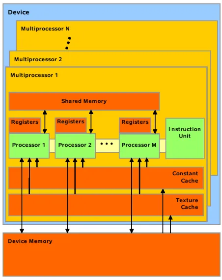
(33) 2.1. The Graphics Hardware. 15. Figure 2.2: The left image shows the CUDA execution process. The right one shows that every block inside the grid is composed by an arbitrary number of concurrent threads. Image taken from [NBGS08]..

(34) 16. Chapter 2. Background. into account especially when current kernel has control flow instructions or uses per block shared memory. All the threads within the same block can cooperate by sharing data and synchronizing their execution in order to access shared memory efficiently. When a synchronize instruction is put in a point in the code, the threads reaching this point wait until all other threads in their same blocks reach it. Then all the threads within a block continue the parallel execution. Since the shared memory is only available at a block level, threads of different blocks cannot synchronize or share information (examples can be found in the following sections). There are strong limitations in the number of threads per block, but a kernel can be executed using a grid with a lot of blocks. This gives us the possibility to have a very large number of threads being executed at the same kernel. In addition to this, the thread cooperation is reduced because the main part of them are actually in distinct blocks. This model allows kernels to run without recompilation on different devices with different hardware capbilities. If the device has very few parallel capabilities it can run all the blocks sequentially. On the other hand, if the device has large parallel capabilities, it will run a lot of them in a parallel fashion. The advantage here is that all these facts are almost totally transparent to the programmer, therefore he can focus his work on improving the algorithms.. Memory model A thread only has access to the device memory, and this space memory is divided into some different memory spaces (see Figure 2.3). The most important ones are explained as follows.. Global memory occupies the main part of the device memory space. It can can be accessed by all the threads within the grid and is not cached (it is the slowest one). The advantage is that it has a lot of space, therefore it might be useful when data is too big to fit in any other kind of memory. All global space memory is accessible from any thread within the grid, thus all the threads of the grid can read or write any position there. Constant memory is a cached small portion (usually 64Kb) of the GPU memory that cannot be modified during the CUDA kernel processing and it is accessible by all the threads. The constant memory is very useful when we have relatively small data.

(35) 2.1. The Graphics Hardware. 17. Figure 2.3: Memory model of CUDA architecture.. that has to be accessed many times by the main part of the threads, because its cache increases the access speed. As its name indicates, we can only read from this space memory. All threads within the grid have access to all the constant space memory. Registers are used by the local variables of each thread. It is a small memory space and a variable located here is only accessible by its thread. On the other hand it is the fastest one. It is important to be careful with this kind of memory because when a thread has occupied all its registers, the next declared variables will be located in the local memory, a portion of memory inside the global memory (the slowest kind of memory inside the GPU). Shared memory is, probably, the most important memory type in CUDA. If the data needed for the CUDA computation must be accessed by distinct threads and a lot of times, the use of shared memory is highly recommended. Shared variables are visible for all the threads within a certain block, thus all data has to be structured in a good way to take advantage of its cache. In fact, the shared memory is the fastest memory space in the GPU..

(36) 18. Chapter 2. Background The global and constant spaces can be set by the host before or after the kernel. execution inside the device. This mechanism is useful for transfering data to the device before the kernel is launched or to host in order to get the results of a previously executed CUDA kernel. A multiprocessor takes 4 clock cycles to issue one memory instruction for a warp. When accessing global memory, there are, in addition, 400 to 600 clock cycles of memory latency. Much of this global memory latency can be hidden by the thread scheduler if there are sufficient independent arithmetic instructions, which can be issued while the global memory access is being complete. Since global memory is of much higher latency and lower bandwidth than shared memory, global memory accesses should be minimized. A typical programming pattern is to stage data coming from global memory into shared memory; in other words, to have each thread of a block: • Load data from device memory to shared memory, • Synchronize with all the other threads of the block so that each thread can safely read shared memory locations that were written by different threads, • Process the data in shared memory, • Synchronize again if necessary to make sure that shared memory has been updated with the results, • Write the results back to device memory.. The CUDA language The CUDA programming interface provides a relatively simple group of primitives for users familiar with the C programming language to program algorithms that can be executed inside the GPU (device). It has extensions to the C language that allow the programmer to target portions of the source code for execution on the device. It also supplies a runtime library composed by: (1) a host component that provides functions to control and access one or more compute devices from the host; (2) a device component providing device-specific functions; (3) a common component with built-in vector types and a subset of the C standard library that are supported in both host and device code..

(37) 2.1. The Graphics Hardware. 19. It is important to remark that only the functions provided by the common runtime component from the C standard library are supported by the device. The following paragraphs describe the basic extensions needed to understand and program CUDA algorithms . Function type qualifiers are the first extension. There are three of them: • A function declared using the __device__ qualifier is always executed on the device and it can only be called from other functions inside it. • The __global__ qualifier is used to create a function that acts as a kernel. A kernel is the main program of a parallel computation running in CUDA. Therefore it can only be executed inside the device and it is always called by the host. • If a function has the __host__ qualifier it is executed on the host and of course, it can only be called from there. It is the default function qualifier. It can be used together with __device__ in order to compile the function for the device and the host and be carried out from both at the same time. Variable type qualifiers are used to specify the memory location of a variable on the device. There are three of them: • The __device__ qualifier declares a variable that resides on the device. The memory space that a variable belongs to, is defined using this qualifier together with the constant and shared ones (see next paragraphs). If none of them is present, then the variable is located in the global memory space, it has the same lifetime as the application and is accessible from all the threads within the grid (from the device) and from the host through the runtime library. • __constant__ qualifier declares a variable that resides in the constant memory space. As with the __device__ qualifier, it has the lifetime of an application and is accessible from all the threads within the grid and from the host through the runtime library. • Finally, __shared__ qualifier declares a variable that resides in the shared memory space of a thread block. It has the lifetime of the block and is only accessible from all the threads within the block. Shared variables are guaranteed to be visible by other threads only after the execution of __syncthreads(). These variable qualifiers are not allowed on struct and union members, on formal parameters and on local variables within a function that is executed on the host..

(38) 20. Chapter 2. Background Variables defined using __shared__ or __constant__ qualifier can not have dynamic storage. __device__ and __constant__ variables are only allowed at file scope. They can not be defined inside a function. As its name says, a __constant__ variable cannot be modified from the device, only from the host through host runtime functions. They are actually constant to the device. Generally a variable declared in device code without any of these qualifiers is automatically put in a register. However in some cases the compiler must choose to place it in local memory (much more slower). This is often the case for large structures or arrays that might consume too much register space or when the register space for a thread is already full. This is also the case of arrays for which the compiler cannot determine if they are indexed with constant quantities.. A new directive to specify how a __global__ function or kernel is executed on the device from the host is needed. This directive specifies the execution configuration for the kernel and it defines, basically, the dimension of the grid and blocks that will be used to execute the function on the device. It is specified by inserting an expression of the form <<< Dg, Db >>> between the function name and the argument list, where: • Dg is of type dim3 and specifies the dimension and size of the grid, such that Dg.x ∗ Dg.y equals the number of blocks being launched; Dg.z is unused or it is always 1. • Db is also of type dim3 and specifies the dimension and size of each block, such that Db.x ∗ Db.y ∗ Db.z equals the number of threads per block. Four built-in variables that specify the grid and block dimensions and the block and thread indices. • gridDim and blockDim are of type dim3 and contain the dimensions of the grid and block respectively. • blockIdx and threadIdx are of type uint3 and contain the block index within the grid and thread index within the block respectively. • warpSize is a variable of type int and contains the warp size in threads. It is not allowed to take the address or assign values to any of them. Each source file containing these extensions must be compiled with the CUDA compiler nvcc that will give an error or a warning on some violations of these restrictions. However,.

(39) 2.2. Computational geometry concepts. 21. in most cases the errors or warnings cannot be automatically detected, thus we must take special care when programming CUDA algorithms.. 2.2. Computational geometry concepts. In this section the geometric concepts and algorithms mainly used in our visibility and good-visibility maps computation are briefly described. One of the most importants topics needed to compute good-visibility maps is the so-called depth contours problem, which treats the problem of how deep a region of the plane or space is with respect to a set of points. The depth contours are based on the convexity and its properties, thus the first subsection describes this concept. In order to compute multi-visibility maps, i.e. an overlay of distinct visibility maps, a little explanation of how the overlay of two or more planar subdivisions can be computed is necessary. Finally, some comments related to the definition and creation of terrains is given.. 2.2.1. Convexity. Let a region R and two points p and q inside R in Rd , with d > 0, R is a convex region if all points belonging to the segment pq are interior to R. If two points p and q exist inside R generating a segment which is partially outside R, then R is not convex. Let a set of points S in Rd , its convex hull CH(S) is defined as the minimal convex region containing every point of S. Basically, the computation of CH(S) consists of finding all the exterior points of S. We say that s ∈ S is not exterior with respect to S if a triangle (p, q, r) exists where p, q, r ∈ S, p, q, r ̸= s and s is inside (p, q, r). Another useful property says that s is exterior to S if and only if a line containing s that leaves all the other points in S at one side exists. If the extremal points of S are known and ordered clockwise, CH(S) can be easily computed as the intersection of the halfplanes defined by the oriented lines constructed from every consecutive pair of points. This is possible because an important property of the halfplanes (hyperplanes when considering any number of dimensions) states that an intersection of any of them always results in a convex region. From 1972, a lot of algorithms to efficiently compute the convex hull of a set of points has been reported. Graham [Gra72] proposed the first convex hull algorithm running on the plane with a O(n log n) worst-case running time. Later, Shamos proved in his Ph.D. thesis [Sha78] that the convex hull problem can be reduced to the sorting one, which.

(40) 22. Chapter 2. Background. has a lower bound of Ω(n log n). After the Graham’s algorithm was published, a lot of others algorithms for computing the convex hull from a set of points in a two-dimensional space were reported, as H. Bronnimann and coworkers expose in [BIK+ 04]. There are also algorithms to compute the convex hull of a set of points in three-dimenional spaces (T. Chan briefly describe some of them in [Cha03]) or even in any dimension using the QuickHull algorithm presented by C.B.Barber et al. in [BDH96].. 2.2.2. Overlay of planar subdivisions. A planar subdivision, also known as planar map, divides the plane using vertices, edges and faces induced by a set of line segments. Overlaying two planar subdivisions produces a new planar subdivision. Since a planar subdivision is configured by a set of line segments, if we want to obtain the overlay of two planar maps M1 and M2 it is necessary to intersect every pair of segments, one for each planar map. It can be useful in a wide range of fields, including for Geographic Information Systems (GIS) or for finding multi-visibility maps from a set of view objects. The overlay of two planar maps can be seen as a specialized version of the twodimensional line intersection problem. This problem has been studied for over twenty-five years. Bentley and Ottmann [BO79] developed the first solution to the line intersection problem in 1979, using a plane sweep algorithm with a computational complexity of O(n log n + k log n) time, where k is the number of intersections found and n the number of segments. This algorithm is not optimal because the lower bound has been proved to be Ω(n log n + k). Later, Chazelle et al. [CE92] presented the first algorithm running in optimal time complexity, however it required O(n + k) space. The first optimal algorithm in both time and space was reported by Balaban in [Bal95], which runs in O(n log n + k) time and requires O(n) space. For the case of the map overlay problem, the intersection problem is actually easier than the general case. This is because we assume that a map is a planar subdivision, so every intersection will be between one segment from the first map and one segment from the second map. This problem was solved in O(n log n + k) time and O(n) space by Mairson and Stolfi [MS87] before the general problem was solved optimally. Moreover, if we assume that planar maps are connected subdivisions, Finke and Hinrichs [FH95] showed in 1995 that the problem can be solved in O(n + k) time..

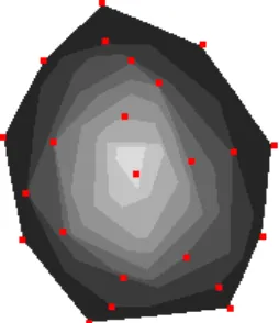
(41) 2.2. Computational geometry concepts. 2.2.3. 23. Depth contours. In this section the depth contour concept is presented. Hereafter its formal definition and some algorithms to compute it on the plane are summarized. Afterwards some implementations using graphics hardware techniques are reported and finally compared with our implementation.. Definition Let P be a set of n points. The location depth of an arbitrary point q relative to P , denoted by ldP (q), is the minimum number of points of P lying in any closed halfplane defined by a line through q. The k-th depth region of P , represented by drP (k), is the set of all points q with ldP (q) = k. For k ≥ 1, the external boundary dcP (k) of drP (k) is the k-th depth contour of P . The depth map of P , denoted dm(P ), is the set of all depth regions of P (see Figure 2.4) whose complexity is O(n2 ). When all points of P are in convex position we achieve the latter complexity, thus this bound is tight.. Figure 2.4: Representation of the depth contours of a set of 23 points.. Depth Contours computation in the plane Miller et al. [MRR+ 03] presented an algorithm for computing the depth contours for a set of points that makes an extensive use of duality, and proceeds as follows: given a set P of points, the algorithm maps all points of P to their dual arrangement of lines. Then, a topological sweep is applied to find the planar graph of the arrangement whose vertices are labeled with their respective levels, i.e. the number of dual lines above them. The depth of a vertex can be computed using min(level(v), n − level(v) + 1). Finally, for a.

(42) 24. Chapter 2. Background. given k, dcP (k) is computed by finding the lower and upper convex hulls of the vertices at depth k. Each of these vertices corresponds to a halfplane in the primal plane. dcP (k) is the boundary of the intersection of the previously mentionned halfplanes. dcP (k) does not exist if this intersection is empty. The complexity of the algorithm is O(n2 ) in time and space, which has been shown to be optimal. Since for large n the running time of Miller et al. algorithm might be too large, in the following section some algorithms are presented that solve the latter problem by using graphics hardware capabilities (i.e. an image of the depth contours is drawn where the color of a pixel represents its depth value).. Graphics Hardware solutions Depth contours have a natural characterization in terms of the arrangement in the dual plane induced by the set P of n points. The mapping from the primal plane Π to the dual plane Π′ is denoted by the operator D(·). D(p) is the line in plane Π′ dual to the point p, similarly D(l) is the point in plane Π′ dual to the line l. We denote the inverse operator by P (·), i.e. P (q) is the line in plane Π primal to the point q in the dual plane Π′ . Each point p ∈ P in the primal plane is mapped to a line l = D(p) in the dual plane (see Figure 2.5). We can also define the dual of a set of points P as D(P ) = ∪p∈P D(p). The set of lines D(P ) define the dual arrangement of P . In this dual arrangement the level of a point x is computed as the number of lines of D(P ) that satisfy the following criteria: they either contain or stricly lie below x (see Figure 2.6). The depth contour of depth k is related to the convex hull of the k and (n − k) levels of the dual arrangement. Krishnan and coworkers [KMV02] and Fisher et al. [FG06] developed algorithms that draw a discretization of the depth contours from a set of points using graphics hardware capabilities. Both algorithms are based on the dual concept. In the first step, the input point set P is converted to a set of lines in the dual plane. The algorithm runs on two bounded duals instead of one, due to the finite size of the dual plane. In that way it is guaranteed that all intersection points between the dual lines lie in one of the two latter dual regions. Since each dual plane is discrete, it is possible to compute the level of each pixel by drawing the region situated above every dual line of P , by incrementing by one the stencil value of the pixels located inside each of these regions. In the second step the two images generated in this fashion are analyzed. For each pixel q located on a dual line, its corresponding primal line P (q) is rendered with the appropriate depth and color as a graphics primitive using the depth test (z-buffer). The complexity in time of the algorithm.