IV Reunión sobre Pobreza y Distribución del Ingreso
Universidad Nacional de La Plata
Universidad Torcuato Di Tella
Universidad de San Andres
Capítulo Argentino de la Red LACEA/BID/Banco Mundial sobre Desigualdad y
Pobreza
Universidad Nacional de La Plata
Facultad de Ciencias Económicas
La Plata, 26 y 27 de Junio de 2003
Trade Reforms, Market Access and Poverty in Argentina
Trade Reforms, Market Access and Poverty in
Argentina
∗
Guido G. Porto
†Development Research Group
The World Bank
February 2003
Abstract
This paper examines the impact of national and foreign trade reforms on poverty in Argentina. National reforms include the removal of Argentine import tariffs. Foreign reforms include the elimination of agricultural subsidies, and tariffs and non-tariff barriers in developed countries (i.e. the United States and the European Union). From a head count ratio of 25.7 percent in 1999, a combination of domestic and global trade liberalization would cause a decline of between 1.6 and 4.6 percentage points in the poverty rate. The marginal effects of national trade reforms are larger than those of foreign trade reforms. However, there is a much greater scope for policy reforms in developed countries. In Argentina, in the end, I find that foreign reforms are more important than national reforms in terms of poverty alleviation.
∗I wish to thank I. Brambilla, B. Hoekman, and M. Olarreaga for continuous support and very valuable comments. All errors are my responsibility.
1
Introduction
Much of the literature that studies the relationship between trade and poverty in developing
countries focuses on the effects ofnational trade reforms, such as own tariffreductions (Porto, 2002; Goldberg and Pavcnik, 2003). In contrast, the WTO negotiations at the Doha Round
were more concerned with the poverty effects, on low-income countries, of foreign reforms, such as the elimination of agricultural subsidies in developed economies. The purpose of this
paper is to empirically compare the relative poverty impacts of national and foreign trade
reforms in Argentina.
The national trade reforms investigated in this paper include tariff cuts on consumption
goods (food, appliances) and capital goods (machines) in Argentina. These policies generate
a decline in the domestic price of these goods. Foreign trade reforms include the elimination,
in developed countries, of agricultural subsidies and trade barriers (tariff and non-tariff) on agricultural manufactures (dairy products, beef, oils) and industrial manufactures (textiles,
transport materials, chemicals). These policies enhance the market access of Argentine
exports and cause an increase in the international (and hence in the domestic) prices of
these goods.
The theoretical links that form the basis of the methodology used in this paper are
simple. The policy induced changes in the prices of traded goods that Argentine consumers
and producers face generate a change in the relative demand of different factors of production,
particularly labor. As a result, wages and household income react and poverty is affected. The estimation of the poverty impacts of trade liberalization comprises three steps. First,
I assess the changes in the prices of imports and exports induced by national and foreign trade
reforms. Second, I estimate wage price-elasticities that measure the responses of Argentine
wages to the price changes. Finally, I use the simulated policy-induced price changes and
the estimated wage price-elasticities to predict the labor income that would hypothetically
be earned by each Argentine household after the reforms. To study the poverty impacts, I
compute pre- and post-policy head-count ratios.1
1The head count ratio is the proportion of the population with an income lower than the poverty line
To compare the relative effects of national and foreign policies, I distinguish themarginal effects of the reforms, i.e. the marginal effect of a trade policy on household income, from the scope for reforms, i.e. the room for further policy changes. In Argentina, I find that national trade reforms have larger marginal effects than foreign trade reforms. However,
since there is greater room for foreign reforms, policy changes in developed countries would
have, in the end, larger poverty impacts.2 Specifically, the joint elimination of Argentine tariffs on consumption goods and capital goods would cause the head count ratio to decline
by between 0.6 and 1.7 percentage points. Foreign policies on agriculture and industry would
lower the poverty rate by between 1.4 and 2.9 percentage points. Overall, a combination of
own reforms and enhanced market access would cause poverty to decline by between 1.7 and
4.6 percentage points. With an actual initial head count ratio of 25.7 percent, this evidence
suggests that trade policies can be important poverty-reducing instruments in Argentina.
The paper is organized as follows. In section 2, I define the poverty indicator, namely the head count ratio, and I use it to characterize the poverty situation in Argentina during
recent years. Section 3 discusses the methodology used to estimate the changes in household
income, the wage price-elasticities, and the poverty measures. Section 4 implements the
methodology using Argentine data and assesses the poverty impacts of national and foreign
trade reforms in the country. Section 5 provides a conclusion offindings.
2
Poverty in Argentina
The poverty measure used in this paper is the head count ratio, HC, defined as the fraction of the population with an income below the poverty line z. That is,
(1) HC = 1
N
[
i
1{yi < z},
where N is the total population and 1{} is an indicator function that takes the value of one if the argument within brackets is true. The poverty line z is the level of income
2In other countries with higher national trade barriers (such as tariff or quantitative restrictions), own
needed to purchase the poverty consumption basket, which includes food items that satisfy
a minimum caloric and energetic intake, and non-food essential items (clothing, housing,
health and education). The poverty line is measured so as to account for the different caloric requirements of individuals with different characteristics, such as sex and age.3 This means
thatz and individual income,yi, are measured in per equivalent adult units (Deaton, 1997). In Argentina, the National Institute of Statistics and Census (INDEC) estimates poverty
lines and per equivalent adult scales (INDEC 2002).
The poverty analysis focuses on the metropolitan area of Buenos Aires, the most
populated urban area in Argentina (comprising around one third of the population of the
country).4 After a peak of 47.3 percent in 1989, due to a hyperinflation episode, the head count ratio decreased until May 1994. Since then, it has steadily increased. In 1992, when
a number of reforms began, the poverty rate fluctuated around 18-19 percent. Whereas in 1999, the baseline period that I use to explore the effects of trade policies, the head count ratio was 25.7 percent.5
Figure 1 plots the density of the logarithm of individual income per equivalent adult (lpai)
in October 1999 (in monthly dollars) in Gran Buenos Aires (GBA). The density is estimated
with standard kernel methods using the optimal bandwidth and a Gaussian Kernel (Pagan
and Ullah, 1999; Silverman, 1986). There are two vertical lines in Figure 1. The rightmost
vertical line at lpai=5.04 (so that income per equivalent adult is $155, around $5 per day)
represents the official poverty line z for October 1999. The area below the density curve and to the left of this poverty line is the proportion of poor people in Buenos Aires, 25.7
percent. The leftmost vertical line at an income per equivalent adult of 65 monthly dollars
represents the indigence line, the expenditure needed to purchase a minimal food bundle
only. In October 1999, 11.3 percent of the population of GBA was living in extreme poverty.
3The reference group comprises adult males. The caloric requirements of other individuals are measured
relative to this reference group (so that, for instance, an adult male requires more calories than an adult female, and children require less calories than adults).
4The reason why I look at Gran Buenos Aires (the metropolitan area) is that, before 2001, poverty lines
were calculated only for this area.
5I chose 1999 as the baseline year to isolate the impact of the recent recession and current crisis. In 2002,
The purpose of this paper is to assess how poverty, as measured by the head count ratio,
is affected by national and foreign trade policies. I do this by predicting the new income
that each Argentine household would earn as a result of a policy change and by comparing
the pre and post policy head count ratios.
3
The Methodology
Conceptually, there are three links in the methodology that I use in this paper. The initial
step is a trade shock, i.e. a national or a foreign trade reform, which causes a change in
the domestic prices of traded goods (exports and imports) in Argentina. The second step is
the response of the labor income of Argentine households, which leads to the third step, the
induced change in the head count ratio. Discussion of these three components follows.
3.1
Changes in the Prices of Traded Goods
The transmission of trade policies to prices is different for different goods. In this paper, I
work with four different products. There are two exportable goods: agricultural manufactures
(dairy products, beef, oils) and industrial manufactures (textiles, chemicals, transport material). There are two importable goods, too: consumption goods (food, appliances) and capital goods (machines). I assume that Argentina is a small open economy that faces exogenously given prices for these goods.
In principle, national and foreign trade policies may affect the domestic prices of both
exports and imports. Whereas the effects of foreign policies are revealed in changes in international prices, national policies introduce a wedge between international and domestic
prices. Since Argentine trade policies mostly involve intervention on imports, I focus on
national trade policies that affect the domestic prices of importable goods. In contrast, I focus on foreign trade reforms that affect the price of Argentine exports for these are the most important policies from the Argentine standpoint.
Argentina, pi g, is
(2) pig =pig∗ψ(τg),
where pi∗
g is the international price and ψ(·) is the function that characterizes the pass-through of national trade policies to domestic prices. To get the price change induced
by a policy reform, I need estimates of this pass-through function, as I discuss in section 4.
For exportable products, let τ∗g be the foreign policy parameter (tariff protection, production support or export subsidies in large developed economies). The domestic price
of an exportable, peg, is
(3) peg =peg∗(τ∗g),
where pe∗
g is the international price, which depends upon the trade policy parameter. In section 4, I discuss how to get estimates of the price change induced by trade policy reforms.
3.2
Changes in Household Income: the Wage Price-Elasticities
This section explains how to measure the changes in household income caused by trade
policies. Let the income of household j, Yj, be
(4) Yj =[ m
wjm+kj,
where wj
m is the wage earned by household member m (head and non-head), and kj is non-labor income, including profits, returns to specific factors and transfers.
Due to data constraints, I am forced to focus on the labor income of all household
members, thus neglecting non-labor income (kj).6 The change in household income caused
6There might be concerns that leaving capital income and profits aside can produce biased results for
by a change in the policy parameterτ∗g that affects the price of an exportable goodpeg is
(5) dYj =[ m
∂wj m
∂pe g
∂pe g
∂τ∗
g
dτ∗g+ ∂k j
∂pg
∂pe g
∂τ∗
g
dτ∗g.
A similar expression can be obtained for the case of a trade policy that affects import prices.
The proportional changes in the total (labor) income of household j is given by
(6) dY j
Yj = [
m
θj mεwjm
∂lnpe g
∂τ∗
g
dτ∗g,
where εwj
m is the elasticity of the wage earned by household member m with respect to the pricepeg, andθ
j
m is the share of the labor income of the membermin total household income. For a policy change fromτ∗
g toτh∗g, the change in the income of householdj, ∆Yj, can be estimated with
(7) ∆gYj =Yj #
[
m
θj meεwj
m $
g
∆lnpe
g(τ∗g;τh∗g),
where ∆glnpe
g(τ∗g;τh∗g) is the predicted change in the price of good g that is caused by the change in policy, and eεwj
m is the estimated wage price-elasticity. Finally, the income of household j after the policy change is given by
(8) Yij =Yj +∆gYj.
A key component of the methodology used here is the estimation of the wage price-elasticities.
In a small open economy, there is a theoretical general equilibrium relationship between
traded good prices and factor prices. In a two-good, two-factor model, this relationship is
established in the Stolper-Samuelson theorem: an increase in the relative price of a traded
good causes a more than proportional increase in the price of the factor intensively used
in its production. For multidimensional models, it is only possible to predict correlations
between movements in factor prices and movements in product prices (Dixit and Norman,
Norman, 1980; Woodland, 1982). Learning the signs and magnitudes of these correlations
becomes an empirical question.
In what follows, I build a general equilibrium model that illustrates how factor prices
(particularly wages) are determined. Equilibrium wages result from the behavior of workers
and firms. The behavior of individual j is represented by the expenditure function, the minimum expenditure needed to attain utility level uj.7 I assume that factor endowments are endogenous (i.e., there is a leisure consumption choice) so that the expenditure function
ej is
(9) ej =ej(p, Lj, uj;χ),
where p is the vector of prices of consumption goods, Lj is the labor supply (hours) and
χ is a vector that represents expenditure shifters, such as household characteristics. It is a
property of this modified expenditure function that the derivative of ej with respect to Lj
gives the supply wage (Dixit and Norman, 1980).
Demand for labor can be obtained from the revenue function πthat shows the maximum
revenue or GDP produced at prices p and factorsv. That is
(10) π =π(p,v,φ),
where φ is a vector of profit-shifters: variables that affect the decisions of firms, technical change. It is a property of the GDP function (Hotelling’s Lemma) that its derivative with
respect to the labor endowment gives the demand wage.
By equating the supply and demand wages, the equilibrium wage wj is defined by
(11) wj =wj(p,v;u;χ,φ),
where u is a vector of utilities.
For the estimation of (11) to be feasible, some structure has to be imposed. In particular,
7I use the expenditure function to derive a theoretical relationship between prices and wages. For the
I assume that the conditions of the factor price insensitivity theorem hold (Feenstra, 2003).
In a model with constant returns to scale, perfect competition and as many traded goods as
factors, wages are fully determined by the prices of the traded goods (which are exogenous).
This is because the system of average cost (zero profit) pricing conditions has a unique solution in factor prices.8 Under these assumptions, (11) simplifies to
(12) wj =wj(p;χ,φ),
which can be estimated with data on wages, prices of traded goods, household characteristics
and controls for technical change.
The approach followed here attempts to recover the wage price-elasticities using household
surveys as a source of data on individual labor income. In Argentina, the necessary data
are available in the Permanent Household Survey (Encuesta Permanente de Hogares, EPH).
The EPHs are labor market surveys with information on wages, employment, hours worked,
and individual and household characteristics.9
The main problem of using survey data to estimate the wage price-elasticities is the lack
of price data at the level of the household. To deal with this, I exploit the time variation
in prices and surveys. In fact, the EPH surveys are gathered in May and October every
year, so that sixteen surveys from 1992 to 1999 (two per year) can be used to identify
the elasticities. This method adapts techniques used in demand analysis. Wolak (1996), for
instance, estimates a system of demand elasticities using the time variation in CPS surveys in
the United States. Similarly, Deaton (1997) develops methods to estimate demand elasticities
using regional variation in unit values. Finally, Goldberg and Tracy (2003) use CPS wage
data and industry specific exchange rates to estimate the factor income effects of exchange rate movements.
The relationship between wages and prices in (12) is possibly different for different types of labor because the response of wages to the same price may depend, in principle, on skill
8See Dixit and Norman (1980) or Woodland (1982) for a detailed analysis of the relationship between
product prices and factor prices. See also Feentra (2003) for a more recent description of the factor price insensitivity model.
intensities. I define three labor factors: unskilled labor (comprising individuals with only primary education), semiskilled labor (comprising individuals having completed secondary
education), and skilled labor (comprising workers holding college degrees).
Let Ej be the 1x3 jth row of a matrix E of dummy variables for the three educational categories of labor. I capture the differential impact of prices on the wages of individuals with different skills with the following model10
(13) logwj =α+[ g
Ejlogpjgβg+Ejγ+zjδ+µj.
In (13),γis the coefficient vector associated with the educational dummies andzj is a vector of individual characteristics, such as age, gender and marital status. The variablelogpj
gis the logarithm of the international price of traded good g (agricultural manufactures, industrial manufactures, imported consumption goods and capital goods).11 In a given time period,
all households face the same prices. The index j attached to the prices in (13) captures the fact that I work with different surveys in time periods with different prices. The estimated
wage-price elasticity for individualj with respect to pricepg is given by Ejfβg. Finally, µj is an error term.
A consistent estimate of the wage elasticities βg requires exogenous domestic prices
and exogenous trade reforms. To solve the problem of potential endogenous policy, I use
the international price indexes as regressors in (13).12 Since for a small open economy
international prices are exogenously given, the regression model estimatesβg consistently.13
In the model specified in (13), equilibrium wages are determined by individual characteristics (to account for the heterogeneity of labor supply) and prices (to account
for labor demand). In addition, I include time trends in the regressions, interacted with the
10This is a varying coefficient model. See Hsiao (1986), Swamy (1971) and Raj and Ullah (1980).
11A number of alternative specifications proved that the model in (13) is robust. Including regional and
sectoral dummies does not affect the results. For presentational simplicity, I decided to estimate (13) directly.
12These prices are published by the Argentine Institute of Statistics and Census (see Appendix 1) 13For consistency, it is required that the pass-through function be uncorrelated to the international price.
educational dummies, that capture technical change that may affect wages differently by skill levels.
Since all households in a given survey sample face the same prices, there may be
correlation in the error terms. This is the clustering problem discussed in Kloek (1981). In
the estimation of the model, I assume that the clustering effects are specific to the time period and the educational category of the individual. I use a robust non-parametric estimation of
the covariance matrix to correct the standard errors of the elasticities.
Table 1 reports the estimated wage price-elasticities. I find that the prices of exportable manufactures, either of agricultural or industrial origin, impact positively on wages for
workers of all skills. In contrast, higher import prices for consumption goods cause wages to
decline. Finally, there is a positive effect of the prices of imported machines on the wages of
Argentine workers indicating that labor substitutes for more expensive machines. For each
of these prices, I find that the estimated elasticities do not vary much by skill levels. The
finding that the wages of skilled and unskilled workers react in the same direction to trade liberalization is perfectly consistent with the theoretical correlations between factor prices
and product prices since I do not restrict the model to display Stolper-Samuelson effects.
The bottom panel of Table 1 reports the coefficients of the time trends, interacted with the educational dummies (so as to measure different types of technical change). The trend
coefficients are positive and increasing in the skill level. These controls thus capture the increasing inequality in the functional distribution of income, a characteristic feature of the
Argentine economy during the 1990s.
3.3
Poverty Impacts
To carry out the poverty analysis, I simply compare the proportion of poor individuals before
counterfactual income,Yhj, of Argentine households, which is defined by (8).
To get the per equivalent scale measure, the counterfactual household income is devided
by the adult scales reported in INDEC (2002). Let Fh(·) be the cumulative distribution function of the log of counterfactual household income yhj generated by the policyhτ.14 The post policy head count ratio is therefore Fh(z). Accordingly, the change in policy τ will be poverty decreasing if
(14) F(z)≥Fh(z).
In this paper, I want to make a distinction between themarginal effect of the reform, i.e. the induced marginal change in the income of the household, and the scope for reforms, i.e. the room for (further) changes in policies. This distinction is crucial to understand the relative
poverty impacts of national and foreign trade reforms in Argentina. To clarify matters, the
change in the head count ratio, ∆HC, is written as
(15) ∆HC=[ i
1yhj < z−[
i
1yj < z.
The marginal effect of a trade policy reform is given by the change in the head count ratio
caused by a small change in the policy parameter. If I estimate these marginal effects by
counting the number of poor people before and after a small policy reform, the head count
ratio will be estimated with a large bias given the small sample that will be affected by the
reform. In this case, it is convenient to estimate the marginal effects using the empirical approximation to the theoretical formula (15). This is given by
(16) ∆gHC= z ]
0 g
f(yh)dhy− z ]
0 g
f(y)dy.
14Note that the change in policy affects not only the distribution function but probably the poverty line,
The densities ofyandyhcan be estimated with standard non-parametric methods (Pagan and Ullah, 1999; Silverman, 1986). At a selected point of the support of the per-equivalent-adult
income,y, the estimated change in the head count ratio is
(17) ∆gHC= 1
nh z ] 0 # [ i K h
yi−y
h
−K
yi−y
h
$
,
whereK is the Kernel,h is the bandwidth andnis the sample size. To estimate the integral in (17), I use numerical integration (Simpson’s rule).15
The scope for trade reform indicates the room policymakers have to introduce further
reforms in an economy. In the case of trade policies, the scope for reforms depends on the
initial structure of protection, which is described in section 4 below.
4
Results
4.1
Marginal E
ff
ects and the Scope for Trade Reforms
Argentina exports goods that are intensive in natural resources and labor, and imports
capital and technology intensive goods. In fact, the major exportable goods in Argentina
are agro-manufactures (beef, dairy products, oils and fats), which, in 1999, accounted for 35.2
percent of total exports. Industrial manufactures (textile, machinery, chemicals) represented
29.9 percent of total exports, primary products (cereals, seed, fresh vegetables and fruits),
22.1 percent, and petroleum manufactures, 12.9 percent. Argentine imports comprise capital
and intermediate goods (59.3 percent), consumption goods (17.6 percent) and accessories to
capital goods (16.5 percent).
The upper panel of Table 2 includes data on the structure of protection of Argentine
imports and exports. These data characterize the scope for trade reforms in Argentina and in the rest of the world. In 1996, Argentina, Brazil, Paraguay and Uruguay implemented
15I construct a grid that equally divides the interval of integration into subintervals. I thenfit a quadratic
MERCOSUR, a regional trade agreement. A common external tariff was adopted and intrazone tariffs were eliminated. In Table 2, the average common external tariffon imported
consumption goods is 13.2 percent. For all of these goods, the intrazone tariff (import tax on Mercosur members) is zero. The average tariff, weighted by import shares, is 10.1
percent. The average common external tariff on Capital Goods (machines) is 12 percent, while intrazone Mercosur trade is fully liberalized. The average tariff on machines, weighted by import shares, is 10.3 percent.
On the export side, Argentina has always faced highly distorted markets for its products,
particularly for those of agricultural origin. For most of these goods, trade intervention takes
the form of a tariffrate quota, a two-tier tariffstructure. Argentina is assigned a quota and imports of goods within this quota pay a relatively low tariff. Out of quota imports are
subject to much higher and often times prohibitive tariffs. There are also a number of
non-tariff barriers, such as sanitary standards and, more importantly, subsidies to domestic production or to exports. All these measures cause international prices to decline and restrict
the market access of Argentine products.
Table 2 provides evidence on the magnitude of the tariffintervention in the United States,
the European Union, and Canada. Tariffs are computed according to the OECD (2000) methodology and include the ad-valorem tariff on in-quota imports, the equivalent tariff on
out-of-quota imports, and the ad-valorem equivalent of specific tariffs. The average tariffon agro-manufactured goods is 6.4 percent in the United State, 18.1 percent in Canada and 21.3
percent in the European Union.16 International markets for agricultural manufactures are
further distorted since many developed countries extensively subsidize agriculture production
and exports. All this evidence indicates that there is great scope for changes in foreign
trade-related policies.
For the industrial manufactures sectors, the average tariff is 6.9 percent in the United
States, 11 percent in Canada and 6.4 percent in the European Union. Protection in developed
16The average tariffon Meat is low in the United States, around 2.7 percent, but it is high in Canada and
countries is evidently lower in these industries.17
I turn now to the estimates of the marginal effects of the reforms, reported in the lower
panel of Table 2. I estimate equation (17) for a small change (of one percent) in each of the
prices of the four traded goods. To facilitate the comparison, I work with poverty-decreasing
changes in prices; given the wage price-elasticities, this means that I work with a small
increase in the prices of agro-manufactures, industrial manufactures and capital goods, and
with a small price decrease in the price of consumption goods. I find that the marginal effects of changes in the prices of imported consumption and capital goods are larger than the marginal effects of exported agricultural and industrial manufactures. This means that
the opportunity for positive poverty impacts are larger, on the margin, on the import side
and on national trade policies. This is conditional on the scope for policy reform, which, as I
showed, is much larger on the foreign trade policy side. The total effects are discussed next.
4.2
The Poverty E
ff
ects of Selected Trade policy Reforms
Foreign Trade Reforms
This section looks at the poverty impacts of foreign trade reforms. I examine the effects of increased market access by means of the elimination of tariff protection on agricultural and
industrial manufactures and the removal of domestic support to production and exports of
agricultural products in developed countries.
I begin with agro-manufactures (dairy products, beef, vegetable oils), the sector in
which Argentina has a strong comparative advantage. For the poverty comparisons, I need
estimates of the changes in international prices brought about by foreign trade policies. Due
to data constraints, these changes are very difficult to estimate. As a consequence, I adopt an
alternative strategy that consists of computing lower and upper bounds for the pass-through
of foreign trade liberalization to prices. These bounds define the limits of the confidence band for the policy induced changes in equilibrium prices.
17Leather manufactures get a 7.6 percent tariffin the United States, a 10.7 percent tariffin Canada and
There are essentially two polar approaches that can be used to estimate price changes:
to recover demand and supply elasticities from the data, or to calibrate a CGE model. The
elasticity methodology is based on the econometric estimation of structural parameters. This
is the correct way to estimate prices changes, but scarcity of data makes its implementation
generally difficult and often times impossible. The CGE modeling, in contrast, relies more on calibration and ad-hoc assumptions and allows for a more thorough computation of economic
responses. I use empiricalfindings on these two strands of literature to define the lower and upper bounds.
One recent paper that estimates the responses of equilibrium prices of agricultural
products in international markets is Hoekman, Ng, and Olarreaga (2003). The authors
estimate the parameters of import demands and export supplies for different goods in
different countries and use these parameters to solve for the equilibrium prices of agricultural
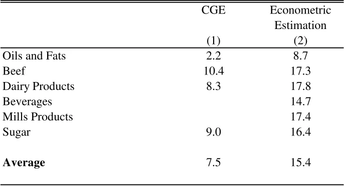
products. Table 3 reports the price changes of the main agro-manufactures products
generated by the elimination of trade protection (tariffs) and domestic support (export
subsidies, production subsidies) in developed countries. The largest price increases are
observed in Dairy Products (17.8 percent), Mills Products (17.4 percent), Beef (17.3 percent)
and Oils and Fats (8.7 percent). Averaging the individual price changes, I get an estimate of
the aggregate price change for agricultural products of 15.4 percent. This defines the upper bound.
Beghin et. al. (2002) perform a CGE study of the responses of the international prices
of agricultural goods to a foreign trade reform that includes the elimination of both trade
protection and domestic support. The authors compute a price increase of 10.4 percent in
Beef, 9 percent in Sugar, 8.3 percent in Dairy Products, and 2.2 percent in Oils and Fats
(see Table 3). The average price change in the price of agro-manufactures is estimated at
7.5 percent. This defines the lower bound.
For each of these lower and upper bounds, I estimate the response of the labor income
of Argentine households. This is simply the product of the wage price-elasticities estimated
in previous sections and the induced change in price. After predicting the hypothetical
policy scenarios. Results are listed in Table 4. The four horizontal panels describe the initial
situation, the poverty impact of foreign reforms, the poverty impacts of national reforms,
and the total poverty effects. Whereas, the four columns show the total population, the total population in poverty, the head count ratio, and the change in the number of poor people.
As of October 1999, 947,570 out of a total of 3.69 million individuals were in poverty
in the metropolitan area of Buenos Aires (GBA). The head count ratio was 25.7 percent.
World trade liberalization in agro-manufactures would cause poverty to decline in Argentina.
For the lower bound of higher prices (7.5 percent), poverty decreases to 901,623 individuals,
from 25.7 percent to 24.4 percent. For the upper bound of higher prices (15.4 percent),
poverty declines to 861,077 people, a 23.3 percent of the population. Based in thesefindings, I conclude that further global trade liberalization in agriculture will be an effective poverty
reducing tool in Argentina, moving between 45,947 and 86,493 people out of poverty.
I turn next to the case of the industrial manufacture sectors, which, in Argentina,
involves textiles, footwear, transport material, and chemicals. The protection granted to
these industries in developed countries is lower than in agriculture, and this is why there are
fewer studies investigating the response of world prices to trade reforms. I therefore adopt a
calibration approach, as follows. Starting from an equilibrium in international markets, the
proportional change in prices (dlnp∗g ) brought about by a tariff change (dln(1 +t)) would be given by
dlnp∗g =− ε
η+εdln(1 +t),
whereε>0is the elasticity of import demand andη >0is the elasticity of export supply of these goods. To help determine the lower bound, I assume a low elasticity of demand of 0.5
and a high elasticity of supply of 2. With an average tariffin developed countries of 8 percent
(see Table 2), prices would increase by approximately 1.6 percent. This is the lower bound
for the price increase. Similarly, a combination of high elasticity of import demand and a
low elasticity of export supply would cause prices to increase by approximately 7 percent.
This defines the upper bound.
is that poverty declines because higher prices for industrial manufactures imply higher wages
for all workers. The head count ratio would decrease from 25.7 percent to 25.5 percent, in
the lower bound, or to 25 percent, in the upper bound. The reduction in the number of poor
people is, however, not trivial, ranging from 5,164 to 23,380 individuals.
Overall, foreign trade reforms would cause a decline in poverty of up to 11 percent, from
an initial head count of 25.7 percent to a post-policy rate of 22.8 percent. Comparing the
lower and upper bounds, there would be from 50,091 to 107,141 fewer poor people in the
country.
National Trade Reforms
Finally, I investigate the implications of eliminating tariff protection on imported consumption and capital goods in Argentina. In Table 2, I reported that the average
protection on these goods is 10.1 and 10.3 percent, respectively. To compute the lower
and upper bound for these prices, I arbitrarily assume a low pass-through rate of 0.2 and
a high pass-through of 0.8.18 The corresponding bounds for the price changes would be 2
percent and 8 percent, respectively.
Results are listed in Table 4. After the elimination of tariffs on consumption goods, the head count ratio would decrease from 25.7 percent to between 24.3 percent and 20.9 percent.
In contrast, cheaper machines (due to lower tariffs) would generate an increase in poverty because firms substitute labor of all skills for capital causing labor demand and wages to decline. In the case of the lower bound, the head count ratio would increase to 26.5 percent;
in the upper bound, the poverty rate would reach 30.2 percent.19
Overall, a full (unilateral) liberalization of trade in Argentina would cause a decline of
poverty from an initial head count ratio of 25.7 percent to 25.1 percent in the lower bound
or to 24 percent in the upper bound. There would be 19,383 fewer poor in the lower bound
scenario and 61,332 fewer poor in the upper bound scenario.
18Given the price data available in Argentina, it is impossible to accurately estimate these pass-through
rates. Nevertheless, I believe these bounds provide a good sense of the likely poverty impacts.
19The analysis only accounts for the short-run effects on poverty, since I do not consider the growth impact
5
Conclusions
This paper has examined the poverty impacts of trade policies. While studies of this kind
tend to focus on the effects of a country’s own trade reforms, here I have looked at the
impact of foreign trade policies as well. Specifically, national reforms included the removal of tariff protection on Argentine imports, and foreign reforms included the elimination of
agricultural subsidies and trade protection so as to enhance the market access of Argentine
exports in developed countries.
To compare these two aspects of trade liberalization, a distinction between the marginal
effects of the reforms (the effects of a small change in policy) and the scope for further
trade reforms (the room for further changes in policy) was made. Although both national
and foreign trade liberalization can significantly reduce poverty in Argentina, I found that foreign reforms are more important than own reforms. The evidence indicates that the
marginal effects on poverty are larger for national policies than for foreign policies, but
that the scope for reforms in developed countries is much larger, both in terms of tariffs protection, non-tariff barriers and domestic support.
To provide an accurate sense of the poverty impacts, I computed a lower bound and an
upper bounds for the price changes and the induced poverty changes. As a lower bound, the
head count ratio would decline from 25.7 percent to 24 percent, or by 1.7 percentage points.
As an upper bound, the head count ratio would decline to 21.1 percent, or by 4.6 percentage
points. Overall, the initial poverty rate would decline by between 6.6 percent and up to 18
percent.
Appendix 1: Data
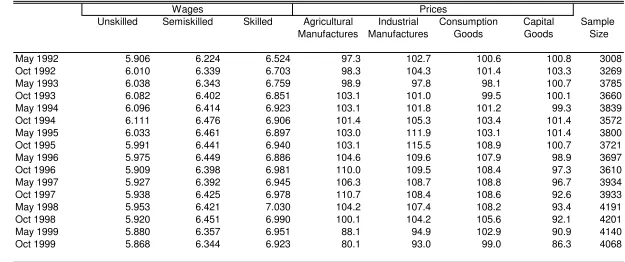
In this Appendix I describe the data that I use to estimate the wage price-elasticities. My method identifies these elasticities using a time series of households surveys and prices. In Argentina, the main source of labor market information is the Permanent Household Survey, Encuesta Permanent the Hogares, or EPH. These surveys are collected in May and October in each year.20 The main source of price data is the National Institute for Statistics and Census (INDEC). The Institute publishes price data on the main exports and import categories in
Argentina. I use the time series of export prices of agricultural and industrial manufactures and the import prices of consumption and capital goods.
The key insight of the empirical methodology is the use of the wage data in the EPHs with the export and import price data. For a given interview period (May or October) in a given year, all households face the same prices. Identification comes from the time variation in prices and surveys. Specifically, I use data from 1992 to 1999, sixteen surveys in total. This strategy is analogous to similar approaches used mainly in demand analysis (Deaton, 1997; Wolak, 1996).
Table A.1 briefly summarizes the data on wages, for different skills, and prices, for exportable and importable products. Sample sizes in each time period are also reported.
References
Beghin, J.C., D. Roland-Holst and D. van der Mensbrugghe (2002). "Global Agriculture
Trade and the Doha Round: What are the Implications for North and South?", Working
Paper 02-WP 308, Center for Agricultural and Rural Development, Iowa State University.
Deaton, A. (1997). The Analysis of Household Surveys. A Microeconometric Approach to Development Policy, John Hopkins University Press for the World Bank.
Dixit, A. and V. Norman (1980).Theory of International Trade. A Dual, General Equilibrium Approach, Cambridge Economic Handbooks.
Feenstra, R.C. (2003). Advanced International Trade: Theory and Evidence", forthcoming,
Princeton University Press, Princeton.
Goldberg, P. and N. Pavcnik (2003). "Trade, Wages, and the Political Economy of Trade
Protection: Evidence from the Colombian Trade Reforms," mimeo, Dartmouth College,
January.
Goldberg, L. and J. Tracy (2003). "Exchange Rates and Wages", Federal Reserve Bank of
New York, mimeo.
Hoekman, B., F. Ng and M. Olarreaga (2002). “Reducing Agricultural Tariffs versus Domestic Support: What is More Important for Developing Countries?”, World Bank Economic Review, forthcoming.
Hsiao, C. (1986). Analysis of Panel Data, Econometric Society Monographs No 11, Cambridge University Press.
INDEC (2002). "Incidencia de la Pobreza y de la Indigencia en los Aglomerados Urbanos",
Press release, Buenos Aires, Argentina.
Jones, R.W. (1965). “The Structure of Simple, General Equilibrium Models,” Journal of Political Economy, Volume 73, Issue 6, December, pp. 557-572.
Judd, K. L. (1998). Numerical Methods in Economics, Cambridge, Massachusetts, MIT Press.
Kloek, T. (1981). “OLS Estimation in a Model Where a Microvariable is Explained by
Aggregates and Contemporaneuos Disturbances are Equicorrelated,”Econometrica, vol. 49, No1, pp. 205-207.
OECD (2000). “Post Uruguay Rounds Tariff Regimes: Achievements and Outlook,” OECD: Paris.
Pagan, A. and A. Ullah (1999). Nonparametric Econometrics, Cambridge University Press.
Porto, G.G. (2002). The Distributional Effects of Trade Policies in Argentina, Ph.D. Dissertation, Princeton University.
Raj, B. and A. Ullah (1981).Econometrics. A Varying Coefficient Approach, London: Croom Helm.
Ravallion, M. (1990). “Rural Welfare Effects of Food Price Changes Under Induces Wage
Responses: Theory and Evidence for Bangladesh,” Oxford Economic Papers 42: 574-585.
Swamy, P.A.V.B. (1971). Statistical Inference in Random Coefficient Regression Models. Berlin: Springer-Verlag.
Wolak, F.A. (1996). “The Welfare Impacts of Competitive Telecommunications Supply: A
Household-Level Analysis,” Brookings Papers on Economic Activity Microeconomics, vol. 1996, pp. 269-340.
Figure 1. Density of per-equivalent-adult Income
est
im
a
te
d
densi
ty
log per-equivalent-adult income
2 3 4 5 6 7 8
Unskilled SemiSkilled Skilled
Prices
Agro-Manufactures 0.75 0.72 0.77
9.66 8.49 6.67
Industrial-Manufactures 0.42 0.24 0.45
1.74 0.99 1.19
Imported -3.10 -2.53 -2.91
Consumption Goods -10.70 -8.03 -6.35
Capital Goods 1.95 2.11 2.21
4.52 4.71 3.51
Trends 0.02 0.03 0.05
5.28 6.97 8.15
[image:25.792.97.644.122.470.2]Notes. Coefficients are in bold and robust t-statistics, in italics. I regress the log of wages on the log of the prices of agro-manufactures, industrial manufactures, imported consumption goods and imported capital goods. The regression includes also a trend interacted with education dummies (to capture technological chance), educational dummies, and inidividual controls such as age, age squared, marital status and gender dummies.
Table 1
Wage Price-Elasticities
Agro Industrial Consumption Capital Manufactures Manufactures Goods Goods
Scope For Reforms
Argentina
Common External Tariff - - 13.2 12.7
Intrazone Tariff - - 0.0 0.0
Rest of the World
United States 6.4 6.9 -
-European Union 21.3 6.4 -
-Canada 18.1 11.0 -
-Domestic Support yes yes
Marginal Effects
Shift in the Distribution
fraction -0.19 -0.10 -0.73 -0.49
total 6879 3612 26962 18119
Notes. The upper panel of the table reports the scope for trade reforms. It includes data on the average import tariff on consumption and capital goods and the average tariff on Argentine exports to developed countries. These averages include the ad-valorem in-quota tariffs, the equivalent out-of-quota tariffs and the equivalent specific tariffs. Data are from OECD (2000). The lower panel of the table shows the marginal effects of trade related events. These are the impacts on poverty of small changes (of one percent) in the prices of the different traded goods. For each of these marginal effects, I report the fraction and the total population affected.
Table 2
Marginal Effecs of Trade Policies and the Scope for Trade Reforms Trade Policies in Argentina and Developed Countries
CGE Econometric Estimation
(1) (2)
Oils and Fats 2.2 8.7
Beef 10.4 17.3
Dairy Products 8.3 17.8
Beverages 14.7
Mills Products 17.4
Sugar 9.0 16.4
Average 7.5 15.4
[image:27.612.134.479.176.362.2]Notes: percentage change in international prices caused by a reform that eliminates all tariff protection and all domestic support on agriculture in developed countries. (1) Beghin et.al. (2002); (2) Hoekman et.al. (2003)
Table 3
Total Population Head Count Change in the Population in Poverty Ratio Number of
(percentage) Poor People
(1) (2) (3) (4)
Baseline
October (1999) 3,691,532 947,570 25.7
FOREIGN REFORMS
Agro-Manufactures
7.5% price increase 901,623 24.4 -45,947
15.4% price increase 861,077 23.3 -86,493
Industrial-Manufactures
1.6% price increase 942,406 25.5 -5,164
7% price increase 924,190 25.0 -23,380
Total
Lower Bound 897,479 24.3 -50,091
Upper Bound 840,429 22.8 -107,141
NATIONAL REFORMS
Imported Consumption Goods
2% price decrease 897,479 24.3 -50,091
8% price decrease 770,896 20.9 -176,674
Imported Capital Goods
2% price decrease 979,577 26.5 32,007
8% price decrease 1,114,468 30.2 166,898
Total
Lower Bound 928,187 25.1 -19,383
Upper Bound 886,238 24.0 -61,332
TOTAL REFORMS
Lower Bound 887,235 24.0 -60,335
Upper Bound 778,033 21.1 -169,537
(1): refers to the total population represented in the sample
[image:28.612.71.500.134.660.2](2): refers to the number of people whose income is below is poverty line (3): refers to the proportion of poor people over the total population
Table 4
Unskilled Semiskilled Skilled Agricultural Industrial Consumption Capital Sample
Manufactures Manufactures Goods Goods Size
May 1992 5.906 6.224 6.524 97.3 102.7 100.6 100.8 3008
Oct 1992 6.010 6.339 6.703 98.3 104.3 101.4 103.3 3269
May 1993 6.038 6.343 6.759 98.9 97.8 98.1 100.7 3785
Oct 1993 6.082 6.402 6.851 103.1 101.0 99.5 100.1 3660
May 1994 6.096 6.414 6.923 103.1 101.8 101.2 99.3 3839
Oct 1994 6.111 6.476 6.906 101.4 105.3 103.4 101.4 3572
May 1995 6.033 6.461 6.897 103.0 111.9 103.1 101.4 3800
Oct 1995 5.991 6.441 6.940 103.1 115.5 108.9 100.7 3721
May 1996 5.975 6.449 6.886 104.6 109.6 107.9 98.9 3697
Oct 1996 5.909 6.398 6.981 110.0 109.5 108.4 97.3 3610
May 1997 5.927 6.392 6.945 106.3 108.7 108.8 96.7 3934
Oct 1997 5.938 6.425 6.978 110.7 108.4 108.6 92.6 3933
May 1998 5.953 6.421 7.030 104.2 107.4 108.2 93.4 4191
Oct 1998 5.920 6.451 6.990 100.1 104.2 105.6 92.1 4201
May 1999 5.880 6.357 6.951 88.1 94.9 102.9 90.9 4140
Oct 1999 5.868 6.344 6.923 80.1 93.0 99.0 86.3 4068
Source: Wage data are from the Permanent Household Survey (EPH). Prices are reported by the National Institute of Statistic and Census (INDEC). The data refer to the price index of the main categories of exports and imports in Argentina.
[image:29.792.77.702.108.370.2]Wages Prices
Table A.1