Fully Discrete Approximations to the Time Dependent Navier–Stokes Equations with a Projection Method in Time and Grad Div Stabilization

Fully discrete approximations to the time-dependent

Navier-Stokes equations with a projection method in

time and grad-div stabilization

Javier de Frutos

Bosco Garc´ıa-Archilla

Julia Novo

May 22, 2019

Abstract

This paper studies fully discrete approximations to the evolutionary Navier– Stokes equations by means of inf-sup stable H1-conforming mixed finite elements with a grad-div type stabilization and the Euler incremental projection method in time. We get error bounds where the constants do not depend on negative powers of the viscosity. We get the optimal rate of convergence in time of the projection method. For the spatial error we get a boundO(hk) for theL2 error of the velocity,

k being the degree of the polynomials in the velocity approximation. We prove numerically that this bound is sharp for this method.

Keywords Incompressible Navier–Stokes equations; inf-sup stable finite element methods; grad-div stabilization; error constants independent of the viscosity; pro-jection methods

1

Introduction

Let Ω ⊂ _Rd_{, d ∈ {2,3}, be a bounded domain with polyhedral and Lipschitz}

boundary∂Ω. The incompressible Navier–Stokes equations model the conservation of linear momentum and the conservation of mass (continuity equation) by

∂tu−ν∆u+ (u· ∇)u+∇p=f in (0, T)×Ω,

∇ ·u= 0 in (0, T)×Ω, (1)

u(0,·) =u0(·) in Ω,

∗_{Instituto de Investigaci´on en Matem´aticas (IMUVA), Universidad de Valladolid, Spain. Research}

supported under grants MTM2016-78995-P (AEI/MINECO, ES) and VA024P17, VA105G18 (Junta de Castilla y Le´on, ES) cofinanced by FEDER funds ([email protected])

†_{Departamento de Matem´atica Aplicada II, Universidad de Sevilla, Sevilla, Spain. Research supported}

by Spanish MINECO under grant MTM2015-65608-P ([email protected])

‡_{Departamento de Matem´aticas, Universidad Aut´onoma de Madrid. Spain Research supported under}

whereuis the velocity field,pthe kinematic pressure,ν >0 the kinematic viscosity coefficient, u0 a given initial velocity, and f represents the accelerations due to

body forces acting on the fluid. The Navier–Stokes equations (1) are equipped with homogeneous Dirichlet boundary conditionsu=0 on ∂Ω.

terms. Different schemes are obtained depending on which stabilization terms are added. For all of them, error bounds with constants independent on inverse powers of ν are obtained in the analysis in [27].

All error bounds in the above mentioned papers may depend implicitly on the viscosity through norms of the solution of the continuous problem on higher order Sobolev spaces. This will be also the case for the present paper and the rest of the related papers which we comment on further below.

In the present paper, we consider as time integrator the Euler incremental projec-tion method. As stated in [38] “For high Reynolds number flows, splitting methods are more efficient computationally and competitive in accuracy compared to the mores expensive coupled methods”. In [31] a subgrid stabilized projection method is applied for the simulation of 2D unsteady flows at high Reynolds numbers. In [8] a pressure-correction scheme for the incompressible Navier Stokes equations combin-ing a discontinuous Galerkin approximation for the velocity and a standard continu-ous Galerkin approximation for the pressure is considered. The method is validated against a large set of classical two- and three-dimensional test cases covering a wide range of Reynolds numbers. In [22] the authors present numerical simulations for incompressible Navier-Stokes equations based on high-order discontinuous Galerkin discretizations and projection methods. The authors state that operator splitting techniques are well established solution approaches for incompressible Navier-Stokes equations that are particularly efficient for high Reynolds number flows. In [9] both sparse and standard grad-div stabilized projection methods are considered. It is shown that grad-div stabilization can increase the accuracy of projection methods for Navier-Stokes equations. As stated in [9] “An important future direction is to study grad-div stabilization, standard and sparse, for turbulent and higher Reynolds number flows, as there appears to be little in the literature on this topic both for projection and coupled time stepping schemes”. Based on all these facts, we con-sider an interesting subject to get error bounds for projection methods applied to the Navier-Stokes equations with constants independent on inverse powers of the viscosity parameter.

An analysis of the semi-discretization in time with the Euler incremental scheme can be found in [42]. On the other hand, the Euler incremental scheme with a spa-tial discretization based on inf-sup stable mixed finite elements and a semi-implicit treatment of the nonlinear term has been analyzed in [33], where the authors get optimal error bounds. In the present paper, we follow the ideas in [33] with the main difference that our aim is to get bounds with constants independent on in-verse powers of the viscosity, which was not intended in [33]. For this purpose, as mentioned above, we add a grad-div stabilization term to the spatial Galerkin discretization. We notice that error constants independent of the viscosity may also imply other practical consequences (besides the obvious one of smaller errors) as the following words from [11] aptly point out: “The importance of stabilization in the high Reynolds number regime from fractional-step methods was illustrated nu-merically in [31] for Navier-Stokes flows, showing that pressure-projection methods can fail to converge in the high Reynolds number regime unless some stabilization is applied”.

in theL2 norm of the velocity, theL2 norm of the divergence of the velocity and a discrete in timeL2 norm of the pressure. Due to the requirement of error constants independent on the Reynolds number, the error in the pressure is obtained under the assumption ∆t ≤ Chd/2+1, k ≥ d/2 + 1, d being the spatial dimension, and

k being the degree of the polynomials in the velocity space, as opposed to [33], where the dependence of error constants on the Reynolds number allow for the weaker assumption ∆t ≤Ch1/2. Numerical experiments in Section 4 suggest that the restriction ∆t≤Chd/2+1 is not sharp in practice and that it is only needed in the proofs due to the technicalities of the analysis. For the spatial error we get a boundO(hk) for theL2 error of the velocity, kbeing the degree of the polynomials in the velocity approximation. This error bound is suboptimal in space compared to other methods in the literature although we prove numerically that the bound is sharp for this method. Assuming enough regularity for the solution, error bounds of size O(hk+1/2) have been proved in [12], [27] using continuous interior penalty stabilization and local projection stabilization, respectively. Although one might expect order k+ 1 for the L2 error of the velocity this is one of the open problems that can be found in reference [37].

Error bounds for projection methods with constants independent of the Reynolds number were also obtained in [11] (which, to our knowledge, it is the first paper analyzing projection methods obtaining such bounds). In [11] the authors proved error bounds for the Euler incremental projection method and the continuous inte-rior penalty finite element method in space with equal order elements for velocity and pressure (analyzed in [13] for stationary Oseen equations). However as opposed to the present paper, error bounds in [11] are obtained for the transient Oseen equa-tions. Also, following [14], in [11] the authors proved a bound for a discrete in time primitive of the pressure instead of the stronger discrete in time L2 norm of the pressure as in the present paper. The idea of getting a bound for the time-average of the pressure error considerably simplifies the pressure error analysis with respect to the standardL2(0, T;L2(Ω)) norm (or its discrete counterpart) in which the pres-sure is usually bounded. Let us observe that in [11], for methods where the prespres-sure is treated explicitly, a condition of type Ch≤∆tis required in the error analysis.

Related to the present paper also is [4], where a method with LPS streamline-upwind stabilization plus grad-div stabilization in space and a BDF2 projection method in time was analyzed. In the first part of [4] error bounds with constants independent on inverse powers of ν are obtained. However, the bounds depend on ku_hk_L∞_(L∞₎, u_h being the approximation to the velocity, and no a priori bounds

for this norm are proved. Moreover, the error bounds for the velocity are only

O(∆t) instead ofO((∆t)2) and no error bounds for the pressure are proved. In the second part of [4] the authors get optimal bounds of orderO((∆t)2) for the velocity (although only O(∆t) for the pressure) although this is done at the price of error constants depending on ν−1.

non inf-sup stable and inf-sup stable elements was analyzed and in the non inf-sup stable case a local projection type stabilization is required. As opposed to this, no stabilization is added in [28], [29], where we obtained error bounds for a modi-fied Euler non-incremental method for non inf-sup stable elements for evolutionary Stokes and Navier-Stokes equations. In [41] a stabilized version of the Euler incre-mental method for non inf-sup stable elements is proposed although no bounds are proved. In [24] the applicability of weighted essentially non-oscillatory (WENO) finite difference schemes for the simulation of incompressible flows is explored in conjunction with several non-incremental and incremental projection methods. A pressure stabilization PetrovGalerkin (PSPG) type of stabilization is introduced in [24] for the incremental schemes to account for the violation of the discrete inf-sup condition. We also want to refer to [32] for an overview on projection methods.

Altogether, in all the mentioned works, apart from [11] and [4], only stability aspects of the methods are studied or error bounds are proved but with constants in the error bounds depending on inverse powers of the viscosity parameter. Then, our aim in this paper is, as in [4], to fill in some sense the existing gap in the numerical analysis of getting bounds for the time-dependent incompressible Navier-Stokes equations with projection methods in time for high Reynolds numbers.

The outline of the paper is as follows. In Section 2 we introduce some notation. In Section 3 we prove the error bounds of the method. The main results are Theorem 1 that gathers the velocity bounds and which statement can be found at the end of Subsection 3.1, and Theorem 2, with the error bound for the pressure, which is located at the end of subsection 3.2. Some numerical results are presented in Section 4.

2

Preliminaries and notation

Throughout the paper,Ws,p_{(D) will denote the Sobolev space of real-valued}

func-tions defined on a domainD⊂_Rd_{,d= 2,3 with distributional derivatives of order}

up to s in Lp(D). These spaces are endowed with the usual norm denoted by k · k_Ws,p_(D). Ifsis not a positive integer,Ws,p(D) is defined by interpolation [1]. In

the cases= 0, it isW0,p(D) =Lp(D). As it is standard,Ws,p(D)dwill be endowed with the product norm and, since no confusion can arise, it will be denoted again by k · k_Ws,p_(D). The casep= 2 will be distinguished by usingHs(D) to denote the

space Ws,2_{(D). The space H}1

0(D) is the closure in H1(D) of the set of infinitely

differentiable functions with compact support inD. For simplicity,k · ks(resp. | · |s)

is used to denote the norm (resp. seminorm) both inHs(Ω) orHs(Ω)d. The exact meaning will be clear by the context. The inner product of L2_{(Ω) or L}2_(Ω)d _will

be denoted by (·,·) and the corresponding norm by k · k0. The norm of the space of

essentially bounded functions L∞(Ω) will be denoted by k · k∞. For vector-valued

functions, the same conventions will be used as before. The norm of the dual space

H−1(Ω) of H₀1(Ω) is denoted by k · k−1. As usual, L2(Ω) is always identified with

its dual, so one hasH₀1(Ω)⊂L2(Ω)⊂H−1(Ω) with compact injection. For a given Banach spaceW,Lp_{(0, T, W) denotes the corresponding Bochner space of functions}

defined on the time interval (0,T) with values in W. The norm inLp(0, T, W) will be denoted byk · k_Lp_(W). When no confusion can arise we will frequently drop the

Using the function spaces V =H₀1(Ω)d and

Q=L2₀(Ω) =q∈L2(Ω) : (q,1) = 0 ,

and assuming that f ∈L2(0, T, H−1(Ω)d), the weak formulation of problem (1) is as follows: Find (u, p) ∈

L2(0, T, V)∩L∞(0, T, L2(Ω)d)

×L2(0, T, Q) such that for all (v, q)∈V ×Q,

h∂tu,vi+ν(∇u,∇v) + ((u· ∇)u,v)−(∇ ·v, p) + (∇ ·u, q) =<f,v>,

with u(0,·) = u0(·) in Ω. Here, h·,·i stands for the duality paring between H01

and H−1. Notice that the above relation has sense with ∂tu ∈ L1(0, T, H−1(Ω)d)

(see e.g.,[19, § 8]). Later, however, (u, p) will be required to be more regular, so thatf will also be more regular. Consequently,h·,·iwill be replaced by (·,·).

The Hilbert space

Hdiv={u∈L2(Ω)d | ∇ ·u= 0,u·n|_∂Ω= 0}

will be endowed with the inner product of L2(Ω)dand the space

Vdiv ={u∈V | ∇ ·u= 0}

with the inner product ofV.

Let Π : L2_(Ω)d _{→ H}div _{be the Leray projector that maps each function in} L2(Ω)donto its divergence-free part (see e.g. [19, Chapter IV]. The Stokes operator in Ω is given by

A : D(A)⊂Hdiv →Hdiv, A=−Π∆, D(A) =H2(Ω)d∩Vdiv.

The following Sobolev’s embedding [1] will be used in the analysis: For 1≤p < d/s

let q be such that 1_q = 1_p −s_d. There exists a positive constant C such that

kvk_Lq0_(Ω)≤Ckvk_Ws,p_(Ω),

1

q0 ≥

1

q, v∈W

s,p_{(Ω). (2)}

If p > d/s the above relation is valid forq0 = ∞. A similar embedding inequality holds for vector-valued functions.

Let Vh ⊂ V and Qh ⊂Q be two families of finite element spaces composed of

piecewise polynomials of degrees at mostkandl, respectively, that correspond to a family of partitions Th of Ω into mesh cells with maximal diameter h. For

simplic-ity, we restrict ourselves to meshes consisting of triangles/tetrahedra although the bounds of the paper equally hold for quadrilaterals/hexahedra. In this paper, we will only consider pairs of finite element spaces satisfying a discrete inf-sup condition,

inf

qh∈Qh

sup vh∈Vh

(∇ ·vh, qh)

k∇vhk0kqhk0

≥β0, (3)

withβ0 >0, a constant independent of the mesh sizeh. Since the error bounds for the pressure depend both on the mixed finite element used and on the regularity of the solution, and in general it will be assumed thatp∈Q∩Hk_{(Ω) withl≥k−1, in}

It will be assumed that the family of meshes is quasi-uniform and that the following inverse inequality holds for each vh∈Vh, see e.g., [17, Theorem 3.2.6],

kvhkWm,p_(K)≤C_invh

n−m−d1_q−1

p

K kvhkWn,q_(K), (4)

where 0≤n≤m ≤1, 1≤q ≤ p≤ ∞, and hK is the size (diameter) of the mesh

cellK ∈ Th.

The space of discrete divergence-free functions is denoted by

V_hdiv={vh∈Vh | (∇ ·vh, qh) = 0 ∀qh ∈Qh},

and byAdiv

h : Vhdiv→Vhdiv we denote the following linear operator

(Adiv_h vh,wh) = (∇vh,∇wh) ∀vh,wh ∈Vhdiv.

Note that from this definition, it follows that forvh ∈Vhdiv,

k(Adiv_h )1/2vhk0 =k∇vhk0, k∇(Adivh )

−1/2_v

hk0=kvhk0.

We also denote byAh : Vh→Vhdiv the linear operator

(Ahvh,wh) = (∇vh,∇wh) ∀vh ∈Vh,wh ∈Vhdiv.

Additionally, two linear operators Ch : Vh → Vhdiv and Dh : L2(Ω) → Vhdiv are

defined by

(Chvh,wh) = (∇ ·vh,∇ ·wh) ∀vh ∈Vh,wh ∈Vhdiv,

(Dhp,vh) =−(p,∇ ·vh) ∀vh∈Vhdiv.

Denoting by πh theH1(Ω) projection onto Qh, one has that form= 0,1:

kq−πhqkm≤Chj+1−mkqkj+1 ∀q ∈Hj+1(Ω), j= 0, . . . , l. (5)

In the error analysis, the Poincar´e–Friedrichs inequality

kvk₀ ≤Ck∇vk₀ ∀v ∈H₀1(Ω)d,

will be used.

In the sequel, Ihu ∈ Vh will denote the Lagrange interpolant of a continuous

functionu. The following bound can be found in [7, Theorem 4.4.4]

|u−Ihu|Wm,p_(K)≤c_inthn−m|u|_Wn,p_(K), 0≤m≤n≤k+ 1, (6)

wheren > d/pwhen 1< p≤ ∞and n≥dwhen p= 1. In the analysis, the Stokes problem

−ν∆u+∇p=g in Ω,

u=0 on ∂Ω, (7)

will be considered. If we denote by (uh, ph) ∈ Vh ×Qh the mixed finite element

approximation to (7) following [30], one has the estimates

ku−uhk1≤C

inf vh∈Vh

ku−vhk1+ν−1 inf qh∈Qh

kp−qhk0

, (8)

kp−phk0≤C

ν inf vh∈Vh

ku−vhk1+ inf qh∈Qh

kp−qhk0

, (9)

ku−uhk0≤Ch

inf vh∈Vh

ku−vhk1+ν−1 inf qh∈Qh

kp−qhk0

. (10)

It can be observed that the error bounds for the velocity depend on negative powers of ν.

For the analysis, we will use a projection of (u, p) into Vh ×Qh with optimal bounds which do not depend on ν. In [25], [26] a projection with this property was introduced. Let (u, p) be the solution of the Navier–Stokes equations (1) with u∈V ∩Hk+1(Ω)d,p ∈Q∩Hk(Ω), k≥1, for t≥0 the pair (u,0) is the solution of the Stokes problem (7) with right-hand side

g=f −∂tu−(u· ∇)u− ∇p.

Denoting the corresponding Galerkin approximation inVh×Qh by (sh, lh), that is

ν(∇s_h,∇v_h)−(lh,∇ ·vh,) + (∇ ·sh, qh) = (g,vh),

for all (vh, qh)∈Vh×Qh, one obtains from (8)–(10)

ku−shk0+hku−shk1≤Chj+1kukj+1, 0≤j≤k, (11)

klhk0≤Cνhjkukj+1, 0≤j≤k, (12)

where the constantC does not depend onν.

Remark 1Assuming that ∂tu∈Hk(Ω)d∩V and considering (7) with

g=∂t(f −∂tu−(u· ∇)u− ∇p) =−ν∇ut,

one can derive an error bound of the form (11) also for∂t(u−sh).

Following [16], one can also obtain the following bound for sh

k∇(u−sh)k∞≤Ck∇uk∞, (13)

whereC does not depend onν. Let us observe that the assumption

u∈L∞(0, T;W1,∞(Ω)d)

is also required in other related references as [12], [3], [26] and [4]. Since kIh(u)k∞≤Ckuk∞ for someC >0, one can write

kshk∞≤ ksh−Ih(u)k∞+kIh(u)k∞≤Cinvh−d/2ksh−Ih(u)k0+Ckuk∞,

where in the last inequality inverse inequality (4) has been applied. Applying (6), (11), (2) and (13) one gets

Alson what follows, Πdiv_h :L2(Ω)d→V_hdivwill denote the so-called discrete Leray projection, which is the orthogonal projection ofL2(Ω)donto V_hdiv

Πdiv_h v,wh

= (v,wh) ∀wh∈Vhdiv.

By definition, it is clear that the projection is stable in theL2(Ω)dnorm: kΠdiv h vk0 ≤

kvk₀ for allv ∈L2(Ω)d. The following well-known bound will be used

k(I−Πdiv_h )vk0+hk(I−Πdivh )vk1 ≤Chj+1kvkj+1 ∀v∈Vdiv∩Hj+1(Ω)d,

for j = 0, . . . , k. This bound follows from the inverse inequality (4), (11) and from the fact k(I −Πdiv_h )vk₀ ≤ kv −whk0 for any wh ∈ Vhdiv and, in particular

k(I −Πdiv

h )vk0 ≤ kv−vhk0, where vh ∈ Vhdiv solves the problem (∇vh,∇wh) =

−(∆v,wh), for allwh ∈Vhdiv (i.e., for someqh ∈Qh, the pair (vh, qh) is the mixed

finite-element approximation to problem (7) with ν= 1 and g=−∆v).

The method that will be studied for the approximation of the solution of the Navier–Stokes equations (1) is obtained by adding to the Galerkin equations a con-trol of the divergence constraint (grad-div stabilization). More precisely, the fol-lowing grad-div method will be considered: Find (uh, ph) : (0, T]→ Vh×Qh such

that

(∂tuh,vh) +ν(∇uh,∇vh) +b(uh,uh,vh)−(ph,∇ ·vh,)

+ (∇ ·uh, qh) +µ(∇ ·uh,∇ ·vh) = (f,vh),

(15)

for all (vh, qh)∈Vh×Qh, withuh(0) =Ihu0. Here, and in the rest of the paper,

b(u,v,w) = (B(u,v),w) ∀u,v,w∈H₀1(Ω)d,

where,

B(u,v) = (u· ∇)v+1

2(∇ ·u)v ∀u,v ∈H

1 0(Ω)d.

Notice the well-known property

b(u,v,w) =−b(u,w,v) ∀u,v,w∈V, (16)

such that, in particular, b(u,w,w) = 0 for all u,w∈ V. Property (16) in combi-nation with the grad-div term plays a crucial role in our error analysis in order to obtain error constants that do not depend on inverse powers of ν. Whether this is possible with other forms of the nonlinear term (see e. g., [15]) do not seem to have a straightforward answer and will be subject of further studies.

3

Euler incremental projection method

the dependence through norms of the theoretical solution). For this reason we add grad-div stabilization to the plain Galerkin approximations. For the error analysis we follow both the bounds in [33] for the analysis of the projection scheme and the techniques in [26] for getting bounds independent on the inverse of the viscosity. We will consider a uniform partition of the time interval [0, T] with step-size ∆t.

Let ˜un_h ∈Vh,un_h ∈Vh+∇Qh,pn_h ∈Qh be defined by

˜

un+1_h −un h

∆t ,vh

!

+ν(∇˜un+1_h ,∇v_h) + (B( ˜un_h,u˜n+1_h ),vh)−(pnh,∇ ·vh)

+µ(∇ ·u˜n+1_h ,∇ ·vh) = (fn+1,vh), ∀vh∈Vh, (17)

(∇ ·u˜n+1_h , qh) =−∆t(∇(pn+1h −p n

h),∇qh), ∀qh ∈Qh, (18)

un+1_h = ˜un+1_h −∆t∇(pn+1_h −pn_h). (19)

Let us observe that from (19)

(un+1_h ,∇qh) = ( ˜u_hn+1,∇qh)−∆t(∇(pn+1_h −pnh),∇qh), ∀qh ∈Qh,

and then applying (18) we get

(un+1_h ,∇qh) = 0, ∀qh∈Qh. (20)

As pointed out in the introduction, the value of the stabilization parameter µ de-pends on the physical units and there is no clear-cut choice for it.

Let us also observe that since Vh ⊂V then ˜unh ∈ Vh satisfies the homogeneous

Dirichlet boundary conditions of the problem. Also, we notice that using (19) in (17) we can express the method in terms of ˜un_h as

˜

un+1_h −u˜n_h ∆t ,vh

!

+ν(∇˜un+1_h ,∇v_h) + (B( ˜un_h,u˜n+1_h ),vh)−(2pnh−pn

−1

h ,∇ ·vh)

+µ(∇ ·u˜n+1_h ,∇ ·vh) = (fn+1,vh), ∀vh ∈Vh,

Let us observe that, following [33], we have an implicit-explicit scheme where the linear viscosity term is implicit and a semi-implicit treatment of the non-linear term is considered. Clearly, the semi-implicit treatment of the non-linear term can be easily implemented compared with the fully-implicit treatment of the non-linear term while, as it will be proved in the analysis, the method does not lose the optimal rate of convergence in time. Although other choices are possible, for example,B(2 ˜un_h−u˜_hn−1,u˜n+1_h ) in (17), for the analysis and for simplicity we choose the simplest form in (17) for which we do not lose the optimal rate of convergence in time. In any case, the reader will find no difficulty in adapting the proofs of the present paper to other kind of extrapolations from previous time steps used frequently in the literature.

In what follows we will denote by

˜

Arguing as in [33] it is easy to get the error equations

˜

en+1_h −e˜n_h ∆t ,vh

!

+ν(∇˜en+1_h ,∇vh) + (B( ˜unh,u˜n+1h )−B(s n

h,sn+1h ),vh)

+µ(∇ ·˜en+1_h ,∇ ·vh)−(2nh−n

−1

h ,∇ ·vh)

= (τ_1,hn+1,vh) + (τ_2,hn+1,vh) + (τ_3,hn+1,∇ ·vh) + (τ_4,hn+1,∇ ·vh), ∀vh ∈Vh, (21)

(∇ ·˜en+1_h , qh) + ∆t(∇(n+1_h −n_h),∇qh) = ∆t(∇τ_5,hn+1,∇qh), ∀qh∈Qh. (22)

where

τ_1,hn+1=un+1_t −s

n+1 h −snh

∆t , τ

n+1

2,h =B(u

n+1_,un+1_)−B(sn

h,sn+1h ),

τ_3,hn+1=−ln+1_h +πh(2pn−pn−1)−pn+1, τ_4,hn+1 =µ∇ ·(un+1−sn+1_h ),

τ_5,hn+1 =−πh(pn+1−pn).

Let us also observe that from (19) it follows that

en_h = ˜en_h−∆t∇(n_h−n_h−1) + ∆t∇τ_5,hn . (23)

3.1

Error bounds for the velocity

The error estimates that we obtain in this section depend on the following constants

L1 =C∞ max

0≤t≤Tk∇u(t)k∞, L2 =C∞0max≤t≤Tku(t)k2, (24)

whereC∞ is the constant in (14),

C0 =CB max

0≤t≤0 ku(t)k 2

∞+ku(t)k22

, (25)

whereCB is the constant in (40) below,

C1 =CT

C0Cs+µ+ 1

µ

max

0≤t≤Tku(t)k 2 k+1+

1

µ0max≤t≤Tkp(t)k 2 k

+C

Z T

0

kut(t)k2kdt, (26)

C2 =C

Z T

0

ku_tt(t)k2₀dt+C0k∇ut(t)k20+k∇pt(t)k20

dt (27)

C3 =C1 µ

Z T

0

kptt(t)k2₀, (28)

C0 being the constant in (25) and C a generic constant depending on Ω and the generic constants in Section 2.

Proposition 1 Let Lˆ denote Lˆ = 1 + 4(L1+L2₂/µ). The following bound holds for

h≤1, ∆t≤1/Lˆ and 0≤tn≤T:

k˜en_hk2₀+ (∆t)2k∇n_hk2₀+ ∆t n

X

j=1

2νk∇˜ej_hk2₀+µk∇ ·e˜j_hk2₀

(29)

≤enL∆tˆ

k˜e0_hk2₀+ ∆tµ

2k∇ ·e˜

0

hk20+ (∆t)2k∇0hk20+C1h2k+C2(∆t)2+C3(∆t)4

.

Remark 2Let us also observe that adding ±sn+1_h to (19) we have

en+1_h = ˜en+1_h −∆t∇(pn+1_h −pn_h), (30)

so that taking the inner product with en+1_h and recalling the orthogonality condi-tion (20) we get

ken+1_h k2₀− k˜en+1_h k2₀+k˜en+1_h −en+1_h k2₀= 0.

Then,ken+1_h k₀ ≤ k˜en+1_h k₀ and any estimate of k˜en+1_h k₀ also holds for ken+1_h k₀. To obtain the above error bounds, we will use the following discrete Gronwall lemma that can be found in [34].

Lemma 1 Let k, B, and an, bn, cn, γn be nonnegative numbers such that

an+k n

X

j=0 bj ≤k

n

X

j=0

γnaj +k n

X

j=0

cj+B, n≥1.

Suppose that kγn < 1, for all n, and set σn = (1−kγn)−1. Then, the following

bound holds

an+k n

X

j=0

bj ≤exp

k n

X

j=0 σjγj

k n

X

j=0 cj+B

, n≥1.

The convergence result in Theorem 1 will be obtained using stability plus con-sistency arguments. The following Lemma shows stability. It has two statements. The second one (35) will follow easily after proving the first one (33), which is the stability for linear problems.

Lemma 2 Let(wn_h)∞_n=0 and(bn_h)∞_n=1 sequences inVh and(ynh)

∞

n=0 a sequence inQh

and(rn)∞_n=1 and(dn)∞_n=1 sequences inH1(Ω)and L2(Ω), respectively, satisfying for allχ_h ∈Vh andφh ∈Qh

wn+1_h −wn_h ∆t ,χh

!

+ν(∇wn+1_h ,∇χ_h) +µ(∇ ·wn+1_h ,∇ ·χ_h)

−(2y_hn−y_hn−1,∇ ·χ_h) = (bn+1_h ,χ_h) + (dn+1,∇ ·χ_h), (31)

where y_h−1 = y_h0. Assume that 0 < ∆t ≤ 1 Then, for n ≥ 1 the following bound holds,

kwn_hk2₀+(∆t)2k∇y_hnk2₀+ ∆t n

X

j=1

2νk∇wj_hk2₀+µk∇ ·wj_hk2₀

≤enL∆t

kw0_hk2₀+ (∆t)2k∇y_h0k2₀ (33)

+ ∆t n

X

j=1

4kbj_hk2₀+ 1

µkd j_k2

0+ 52k∇rjk20+ 33k∇rj

−1_k2 0

,

where L = 1. Furthermore, if, on the right-hand side of (21), bn+1_h is replaced by

bn+1_h +gn(wn_h,wn+1_h ), wheregn:Vh×Vh →L2(Ω)dsatisfies that for someL1, L2 >0

|(gn_(y

h,vh),vh)| ≤L1kyhk0kvhk0+L2k∇ ·yhk0kvhk0, n≥0, (34)

holds for ally_h,vh∈Vh, then, the following bound holds

kwn_hk2₀+(∆t)2k∇y_hnk2₀+ ∆t n

X

j=1

2νk∇wj_hk2₀+µk∇ ·wj_hk2₀

≤enL∆tˆ

kw0_hk2₀+µ

2∆tk∇ ·w

0

hk20+ (∆t)2k∇yh0k20 (35)

+ ∆t n

X

j=1

4kbj_hk2₀+ 2

µkd j_k2

0+ 52k∇rjk20+ 33k∇rj

−1_k2 0

,

where Lˆ = 1 + 4(L1+L2₂/µ).

The proof of the Lemma can be found in the Appendix.

The estimation of the truncation errors (except that of τ2,h) is given in the

following result

Lemma 3 The truncation errors satisfy the following bounds:

kτ_1,hn k2₀≤Ch 2k

∆t

Z tn

tn−1

ku_t(t)k2_k dt+C∆t

Z tn

tn−1

ku_ttk2₀ dt, (36)

kτ_3,hn k2₀≤Ch2k

max

0≤t≤Tkuk 2

k+1+ max 0≤t≤Tkp(t)k

2 k

+ (∆t)3

Z tn+1

tn−1

kpttk2₀dt, (37)

kτ_4,hn k2₀≤Cµ2h2kkunk2_k+1, (38)

k∇τ_h,5n k2₀≤C∆t

Z tn

tn−1

k∇ptk2₀dt. (39)

Proof For the first one we have

τ_1,hn = (u

n_−sn

h)−(un

−1_−sn−1 h )

∆t +

un_t −u

n_−un−1

∆t

= 1

∆t

Z tn

tn−1

(u−sh)t(t) dt+

1 ∆t

Z tn

tn−1

Applying (11) and Cauchy-Schwarz the first estimate (36) follows. To estimate τ3,h we write

πh(2pn−pn−1)−pn+1= (πh−I)(2pn−pn−1) + 2pn−pn−1−pn+1.

By writing

2pn−pn−1−pn+1=− (pn+1−pn)−(pn−pn−1)

=−

Z tn+1

tn

ptdt+

Z tn

tn−1

ptdt

=−

Z tn+∆t/2

tn−∆t/2

Z t+∆t/2

t−∆t/2

pssds

dt.

and applying (12), (5) and H¨older’s inequality one obtains the estimate (37). The bound τ4,h is a direct consequence of (11). Finally, for τh,5 we may write,

using theH1 stability of the projection πh,

k∇τ_h,5n k2 =k∇πh(pn−pn−1)k2₀≤Ck∇(pn−pn−1)k2₀=C

Z tn

tn−1

∇ptdt

2

0 ,

so that applying H¨older’s inequality the estimate (39) follows

To bound the truncation error τ2,h we will apply the following lemma.

Lemma 4 There exists a positive constantCB such that the following bound holds

kB(un+1,un+1)−B(sn_h,sn+1_h )k₀

≤CB kukL∞_(L∞_(Ω)d₎+kuk_L∞_(H2_(Ω)d₎

kun_−sn

hk1+kun+1−sn+1_h k1

+(∆t)1/2

Z tn+1

tn

k∇utk20 dt

1/2

(40)

Proof We decompose

kB(un+1,un+1)−B(sn_h,sn+1_h )k0 ≤kB(un+1−un,un+1)k0+kB(un−snh,sn+1h )k0

+kB(un,un+1−sn+1_h )k0.

For the first term on the right-hand side above applying (2) we write

kB(un+1−un,un+1)k0=k(un+1−un)· ∇uk0≤ kun+1−unkL2dk∇un+1k_L2d/(d−1)

≤Ckuk_L∞_(H2_(Ω)d₎k∇(un+1−un)k₀

≤Ckuk_L∞_(H2_(Ω)d₎(∆t)1/2

Z tn+1

tn

k∇utk20 dt

1/2

.

For the other two terms arguing similarly we get

kB(un−sn_h,sn+1_h )k0+kB(un,un+1−sn+1_h )k0 ≤ kun−snhkL2dk∇sn+1_h k_L2d/(d−1)

+1

2k∇ ·(u

n_−sn

h)k0ksn+1_h k∞+kunk∞kun+1−sn+1_h k1

≤C k∇sn+1_h k_L2d/(d−1)+ksn+1_h k∞+kunk∞ kun−sn_hk1+kun+1−sn+1_h k1

Recall that ksn+1_h k∞ has ben estimated in (14). To estimate k∇s_hn+1k_L2d/(d−1) we

write

∇sn+1_h =∇(sn+1_h −Ih(un+1)) +∇(Ih(un+1)−un+1) +∇un+1,

so that applying (4), (11), and (6) we have

k∇(sn+1_h −Ih(un+1))k_L2d/(d−1) ≤Ch−1/2k∇(sn+1_h −un+1)k0 ≤Ch1/2kun+1k2

k∇(Ih(un+1)−un+1)kL2d/(d−1) ≤Ch1/2kun+1k2,

and then, applying also Sobolev’s inequality (2) if follows that

k∇sn+1_h k_L2d/(d−1) ≤Ch1/2kun+1k₂+k∇un+1k_L2d/(d−1) ≤C(h1/2+ 1)kun+1k₂. (41)

and the conclusion is reached.

Applying Lemma 4 and (11) we get

kτ_2,hn k2₀ ≤ CB kuk2_L∞_(L∞_(Ω)d₎+kuk2_L∞_(H2_(Ω)d₎

kun−sn_hk2₁+kun−1−sn_h−1k2₁

+∆t

Z tn

tn−1

k∇u_tk2₀ dt

≤ C0

Csh2k(kunk2k+1+kun

−1_k2

k+1) + ∆t

Z tn

tn−1

k∇utk20 dt

. (42)

whereCs and C0 are the constants in (11) and (25), respectively.

Proof of Proposition 1. We will apply Lemma 2 to the error equations (21–22), that is, in Lemma 2 we take wn_h = ˜en_h,y_hn =n_h, bn_h =τ_1,hn +τ_2,hn , d_hn =τ_3,hn +τ_4,hn ,

r_hn=τ_h,5n and

gn(y_h,vh) =B(yh,sn+1h ) +B( ˜u n h,vh),

since, an easy calculation shows

B( ˜un_h,u˜n+1_h )−B(sn_h,sn+1_h ) =B(˜en_h,sn+1_h ) +B( ˜un_h,˜en+1_h )

=gn(˜en_h,e˜n+1_h ).

Prior to applying Lemma 2 we must check that condition (34) holds. For that purpose, using the skew-symmetric property of the nonlinear term (16), we can write

(gn(y_h,vh),vh) = (B(yh,sn+1h ),vh)

≤ k∇sn+1_h k∞kyhk0kvhk0+

1

2k∇ ·yhk0ks

n+1

h k∞kvhk0.

so that applying the estimates (14) it follows that

(gn(y_h,vh),vh) =L1kyhk0kvhk0+L2k∇ ·yhk0kvhk0,

where L1 and L2 are the constants in (24). Thus, we can apply (35) to the error

equations (21–22). Let us observe that the assumption y_h−1 = y0_h is in our case

−_h1 =0_h. This means we take ˜u0_h =u0_h so that equation (22) holds for n+ 1 = 0 with−_h1=0

h and r0h =τ5,h0 = 0.

Thus, applying (35) to (21–22) and taking into account the estimates (36)–(39)

We now state the main result of this section, whose proof is a direct consequence of the estimate (11), Remark 2 and Proposition 1. For simplicity we setu0 = ˜u0 =

sh(0) andp0_h =πhp(0), but, in view of Proposition 1, the reader will find no difficulty

in proving error bounds corresponding to different initial conditions.

Theorem 1 Let Lˆ denote Lˆ = 1 + 4(L1 +L2₂/µ) and set u0 = ˜u0 = sh(0) and p0_h =πhp(0). Then, the following bound holds forh≤1, ∆t≤1/Lˆ and0≤tn≤T:

kun_h−u(tn)k20+k˜unh−u(tn)k20+ ∆t n

X

j=1

µk∇ ·u˜n_hk2₀

≤2 C_s2(2 +µT) +eLTˆ

C1h2k+ 2e ˆ LT _C

2(∆t)2+C3(∆t)4

.

3.2

Error bounds for the pressure

Observe that from (23) we get

en+1_h −en_h

∆t −

˜

en+1_h −˜en_h

∆t =−∇(

n+1 h −2

n h+n

−1

h ) +∇(τ n+1 5,h −τ

n 5,h)

so that adding this equality to (21) we have

en+1_h −en h

∆t ,vh

!

+ν(∇˜en+1_h ,∇v_h) + (B( ˜un_h,u˜n+1_h )−B(sn_h,sn+1_h ),vh)

+µ(∇ ·e˜n+1_h ,∇ ·vh)−(n+1h ,∇ ·vh) =

(τ_1,hn+1,vh) + (τ2,hn+1,vh) + (ˆτ3,hn+1,∇ ·vh) + (τ4,hn+1,∇ ·vh), ∀vh ∈Vh, (43)

where ˆτ_3,hn+1 =−ln+1_h + (πh−I)pn+1, which, applying (5) and (12) can be bounded

as

kˆτ_3,hn k2₀ ≤C max

0≤t≤Th 2k_kuk2

k+1+Ch2k max

0≤t≤Tkp(t)k 2

k. (44)

The errorn+1_h will be estimated by applying the inf-sup condition to (43). This, in turn will require the estimation of a negative norm of (en+1_h −en

h)/∆t, for which

the following result will be needed.

Lemma 5 Let f ∈L2 satisfying

(f,∇qh) = 0, ∀qh∈Qh,

then the following bound holds

kfk−1 ≤Ck(Adivh )−1/2Πdivh fk0+Chkfk0. (45)

Proof We argue as in [5, Lemma 3.11]. Forϕ∈H₀1 we decompose ϕ= Πϕ+∇ξ, for someξ∈H2. Then it holds, (see e.g. [19])

kΠϕk₁ ≤Ckϕk₁, k∇ξk₁ ≤Ckϕk₁.

Then (f, ϕ) = (f,Πϕ) + (f,∇ξ). On the one hand

And, on the other

(f,∇ξ) = (f,∇(ξ−IQ_hξ))≤Chkfk0kϕk1,

whereIQh is the standard interpolant inQh. Then

kfk−1 ≤Chkfk0+CkA−1/2Πfk0. (46)

Finally, to reach (45) we apply [5, (2.15)]

kA−1/2Πfk0 ≤Chkfk0+k(Adivh )

−1/2_Πdiv

h fk0, f ∈L2. (47)

Inserting (47) into (46) the conclusion is reached.

Lemma 6 There exist a positive constant C such that the following bound holds:

β0kn+1_h k0 ≤ Ch

˜

en+1_h −˜en_h ∆t

0

+Cνk∇˜en+1_h k₀+Cµk∇ ·˜en+1_h k₀

+CkB( ˜un_h,u˜n+1_h )−B(sn_h,sn+1_h )k−1 (48)

+Ckτ_1,hn+1k−1+Ckτ_2,hn+1k−1+Ckˆτ_3,hn+1k0+Ckτ_4,hn+1k0.

The proof of the Lemma can be found in the Appendix.

Now, the only term on the right-hand side of (48) whose bound is not standard is the first one. To estimate its value, we will draw ideas from [33]. Let us denote by

dtvn+1=vn+1−vn.

We notice that the first term on the right-hand side of (48) can be written as kdte˜n_hk0/∆t. We will estimate its value by applying Lemma 2 to the following set of equations, which can be obtained by subtracting the expressions corresponding tonand n−1 (21) and (22):

dt˜en+1_h −dte˜nh

∆t ,vh

!

+ν(∇dt˜en+1h ,∇vh) + (B( ˜unh,u˜n+1h )−B(s n

h,sn+1h ),vh)

−(B( ˜un_h−1,u˜n_h)−B(sn_h−1,sn_h),vh) (49)

+µ(∇ ·dt˜en+1_h ,∇ ·vh) + (2dt(nh−n

−1

h ),∇ ·vh)

= (dtτ_1,hn+1,vh) + (dtτ_2,hn+1,vh) + (dtτ_3,hn+1,∇ ·vh) + (dtτ_4,hn+1,∇ ·vh), ∀vh∈Vh,

(∇ ·dte˜n+1h , qh) =−∆t(∇(dtn+1h −dtnh) ,∇qh) + ∆t(∇dtτ5,hn+1,∇qh), (50)

∀qh ∈Qh.

Lemma 7 There exists a positive constant C such that the following bound holds

kdtτ1,hn k20 ≤C(∆t)

h2k

Z tn

tn−2

ku_ttk2_kdt+ (∆t)2

Z tn

tn−2

ku_tttk2₀dt

, (51)

kdtτ_3,hn k2₀ ≤C(∆t)h2k

Z tn

tn−1

kutk2k+1dt+

Z tn

tn−2

kptk2_kdt

+C(∆t)3

Z tn

tn−3

kpttk20dt, (52)

kdtτ_4,hn k2₀ ≤C(∆t)h2kµ2

Z tn

tn−1

kutk2k+1, dt (53)

kdt∇τh,5n k2 ≤C(∆t)3

Z tn

tn−2

kpttk21dt. (54)

Proof Similarly to the estimation ofτ_3,hn in Lemma 3, we may write

dtτ3,hn =

Z tn

tn−1

∂t

lh(t) + (πh−I)(2p(t)−p(t−∆t))

dt+ 2pn−1−pn−2−pn

− 2pn−2−pn−3−pn−1

.

The last two terms have already been estimated in (37). For the first one, applying H¨older’s inequality, (12) and (5), itsL2 _{norm can be bounded by}

(∆t)1/2hk

Cs

Z tn

tn−1

ku_tk2 k+1dt

1/2

+C

Z tn

tn−2

kptk2kdt

1/2

,

so that (52) follows easily. With similar arguments the estimate (53) can be otained. Fordtτ5,h we write

kdt∇τ_h,5n+1k2 =kdt∇πh(pn+1−pn)k20 ≤Ck∇dt(pn+1−pn)k20

=Ck∇(pn+1−2pn+pn−1)k2₀,

and the bound is obtained with arguments similar as those used withτ3,h. Finally,

fordtτ1,h we write

dtτ1,hn =

Z tn

tn−1

(u−sh)t(t)−(u−sh)t(t−∆t)

∆t +

utt(t)−

ut(t)−ut(t−∆t)

∆t

dt

and the bound (51) is obtained by arguing as in the proof of (36).

The following result is a direct consequence of the previous lemma.

Lemma 8 The following bound holds for n≥2:

∆t n

X

k=2

(kdtτ_1,hk k2₀+kdt∇τ_h,5k k2₀+kdt∇τ_h,5k−1k2₀

+1

µ∆t n

X

k=2

(kdtτ_3,hk k2₀+kdtτ_4,hk k2₀

where

ˆ

C1 =

Z T

0

kuttk2k+

µ+ 1

µ

kutk2k+1+

1

µkptk 2 k

dt, (55)

ˆ

C2 =

Z T

0

ku_tttk2₀+kpttk21+

1

µkpttk 2 0

dt. (56)

For the truncation error dtτ2,h we have the following result

Lemma 9 The following bound holds for n≥2:

∆t n

X

k=2

(kdtτ2,hk k20≤C(∆t)2( ˆC3h2k+ ˆC4(∆t)2),

where

ˆ

C3=kuk2_L∞_(H2₎ Z T

0

kutk2k+1dt+kuk2L∞_(Hk+1₎ Z T

0

kutk22dt, (57)

ˆ

C4=kutk2_L∞_(H1₎ Z T

0

ku_tk2

2dt+kuk2L∞_(W1,∞₎

Z T

0

ku_ttk2

2dt. (58)

The proof of the Lemma can be found in the Appendix.

In order to apply Lemma 2 to equations (49–50) we need to rewrite the nonlinear terms in (49), B( ˜un_h,u˜n+1_h )−B(sn_h,sn+1_h )−(B( ˜un_h−1,u˜n_h)−B(sn_h−1,sn_h)). For that purpose, by adding±B( ˜un_h,sn+1_h ) and ±B( ˜un_h−1,sn

h) we write

B( ˜un_h,u˜n+1_h )−B(sn_h,sn+1_h )−(B( ˜un_h−1,u˜n_h)−B(sn_h−1,sn_h)) =

B(˜en_h,sn+1_h ) +B( ˜un_h,˜en+1_h )−(B(˜en_h−1,sn_h) +B( ˜un_h−1,e˜n_h) =

B(˜en_h,sn+1_h )−B(˜en_h−1,sn_h)+ B( ˜u_hn,e˜n+1_h )−B( ˜u_hn−1,e˜n_h). (59)

For the first term on the right-hand side of (59), by adding ±B(˜en_h,sn_h) we write

B(˜en_h,sn+1_h )−B(˜en_h−1,sn_h) =B(dt˜enh,snh) +B(˜enh, dtsn+1_h ),

and, for the second term on the right-hand side of (59), by adding±B( ˜un_h,˜en_h), and then, ±B(dtsnh,e˜nh)

B( ˜un_h,˜en+1_h )−B( ˜un_h−1,˜en_h) =B(dtu˜nh,˜enh) +B( ˜unh, dt˜en+1h )

=B(dt˜en_h,˜en_h) +B( ˜un_h, dt˜en+1_h ) +B(dtsn_h,˜en_h).

Let us denote

gn(vh,wh) =B(vh,snh) +B(vh,˜enh) +B( ˜unh,wh) =B(vh,u˜nh) +B( ˜unh,wh) (60)

τ_h,6n+1 =B(˜en_h, dtsn+1h ) +B(dtsnh,˜enh),

so that the nonlinear terms in (49) can be expressed as

Our next step is to show that gnsatisfies the hypothesis of Lemma 2. This will be accomplished with Lemma 10 below. We need to fix some notation first. Let us denote byC4,L0₁ and L0₂ the following quantities:

C4=eLT /2ˆ (C1+C2+C3)1/2. (61)

L0₁ =C(C4+kuk_L∞_(W1,∞_(Ω)d₎), L0₂ =C(C4+kuk_L∞_(H2_(Ω)d). (62)

where ˆL is that constant in Proposition 1, and C1,C2 and C3 are those defined at

the beginning of Section 3.1.

Lemma 10 Assume thath≤1, ∆t≤1 and that the following condition holds,

∆t≤Chd/2+1, k≥d/2 + 1. (63)

Then, the functionsgn_{defined in (60) satisfy the following bound forn= 2, . . . , N =} T /∆t:

(gn(vh,wh),wh)≤L01kvnhk0kwhk0+L02k∇ ·vhk0kwhk0,

whereL0₁ and L0₂ are the constants defined in (62).

Proof Using the skew-symmetry property of the nonlinear terms we have

(gn(vh,wh),wh) =(B(vh,u˜nh),wh)

≤k∇˜un_hk∞kvnhk0kwhk0+

1

2k∇ ·vhk0ku˜

n

hk∞kwhk0. (64)

We now observe that applying (4) and (14), one finds forj = 1, . . . , N

ku˜j_hk∞≤ k˜ej_hk∞+ksj_hk∞≤Ch−d/2k˜ej_hk0+ksj_hk∞≤C

h−d/2k˜ej_hk0+ku(tj)k2

≤C

h−d/2eLtˆj/2_(C1hk_{+ ∆t(C2+ (∆t)}2_C3))1/2_+ku(tj)k 2

,

where in the last inequality we have applied (29). Assuming h−d/2hk ≤ C and

h−d/2∆t≤C we can write

ku˜j_hk∞≤C(C4+ku(tj)k2), (65)

where C4 is the constant defined in (61). Arguing similarly, applying again (4) and (14), we also get

k∇u˜j_hk∞≤ k∇˜e_hjk∞+k∇sj_hk∞≤C

h−d/2−1k˜ej_hk0+k∇u(tj)k∞

.

Assumingh−d/2−1+k≤C andh−d/2−1∆t≤C we get

k∇˜uj_hk∞≤C(C4+k∇u(tj)k∞). (66)

Now, the statement of the Lemma follows from (64), (65) and (66).

Remark 3Observe that condition (63) means that for d= 2 we need ∆t=O(h2₎

and k ≥ 2 to get the error bounds for the pressure and even stronger conditions ford= 3 (bounds valid from cubics and with ∆t=O(h5/2)). Thus, assuming (63) from (64) it follows that

Lemma 11 Let ˆL0 denote ˆL0 = 1 + 4(L0₁ + (L0₂)2/µ), where L0₁ and L0₂ are the constants defined in (62). Then, in the conditions of Lemma 10, the following bound holds

kdt˜enhk20+ (∆t)2k∇dtnhk20 ≤Ce ˆ L0tn

kdt˜e1hk20+ µ

2∆tk∇ ·dt˜e

1

hk20+ (∆t)2k∇dt1hk20

+ (∆t)2

ˆ

C1+ ˆC3h2k+ C2ˆ + ˆC4)(∆t)2

(67)

+ (∆t)2h−2eLTˆ C1h2k+ (C2+C3)(∆t)2C5

,

where

C5 =

Z T

0

ku_tk2₂dt. (68)

Proof We apply Lemma 2 to (49–50) withwn_h =dte˜n+1_h ,y_hn=dtn+1_h ,gn defined in (60),

bn_h =dtτ_h,1n+1+dtτ_h,2n+1+τ_h,6n+1, d_hn=dtτ_h,3n+1+dtτ_h,4n+1, and rn_h =dtτ_h,5n+1.

In view of the Lemmas 8, 9 and 10, we only need to bound

τ_6,hk+1=B(˜ek_h, dtsk+1_h ) +B(dtskh,˜ekh).

For that purpose we write

kτ_6,hk+1k0 ≤ Ck˜ekhkL2dk∇dtsk+1_h k_L2d/(d−1)+

1 2k∇ ·˜e

k

hk0kdtsk+1_h k∞

+k∇˜ek_hk₀kdtskhk∞+k˜ekhkL2dk∇ ·d_tsk_hk_L2d/(d−1).

Using inverse inequality (4), the estimate of k˜ek_hk₀ in (29), H¨older’s inequality and Sobolev’s inequality (2), we get

kτ_6,hk+1k2

0 ≤ C(h−(d−1)+h−2)k˜ekhk20∆t

Z tk+1

tk

ku_tk2 2dt

≤ Ch−2eLtˆ k

C1h2k+ (∆t)2(C2+ (∆t)2C3)

∆t

Z tk+1

tk

ku_tk2₂dt.

Multiplying by ∆t and summing from k= 1 onwards we have

∆t n

X

k=2

kdtτ_6,hk k2₀ ≤Ch−2(∆t)2eLTˆ

C1h2k+ (C2+C3)(∆t)2

Z T

0

kutk22dt,

and the proof is finished.

Now, we need to bound the initial errors in the first line in (67). We can assume ˜

Lemma 12 Assumeu˜0_h = ˜u0_h =s0_handp0_h =πhp0, so thatdt˜e1h= ˜e1anddt1h =1h.

Then

kdt˜e1_hk2₀+ ∆tµk∇ ·dte˜_h1k2₀+ (∆t)2k∇dt1_hk2₀ (69)

≤C(∆t)2 (1 +µ)(1 +h−2)C1+C0kutkL∞_(Hk₎

)h2k

+ kutkL∞_(H1₎+ku_ttk_L∞_(L2₎+C2+h−2∆tC3

(∆t)2

.

Proof From (21) withn= 0 and takingvh = ˜e1h and applying inverse inequality

(4) we get

k˜e1_hk2₀+ ∆tνk∇˜e1_hk2₀+ ∆tµk∇ ·˜e1_hk2₀ ≤∆t|(B( ˜u0_h,u˜1_h)−B(s0_h,s1_h),e˜1_h)|

+ ∆tk˜e1_hk0(kτ1,h1 k0+kτ2,h1 k0+Cinvh−1(kτ3,h1 k0+kτ4,h1 k0)).

Now, let us observe that

(B( ˜u0_h,u˜1_h)−B(s0_h,s1_h),˜e1_h) = (B(˜e0_h,s1_h),˜e1_h) + (B( ˜u0_h,˜e1_h),˜e1_h) = 0,

since we have assumed e0_h = 0 and used the skew-symmetric property of the non-linear term (16). Then, we can easily get

1 2k˜e

1

hk20+ ∆tνk∇˜e1hk20+ ∆tµk∇ ·e˜1hk02≤C(∆t)2(kτ1,h1 k20+kτ2,h1 k20)

+C(∆t)2h−2(kτ_3,h1 k2

0+kτ4,h1 k20). (70)

Forτ_1,h1 and τ_2,hn from (36) and (42) we deduce

kτ1,hk0 ≤ ChkkutkL∞_(Hk₎+ ∆tku_ttk_L∞_(L2₎,

kτ2,hk0 ≤ C1hk+C0∆tkutkL∞_(H1₎

and, thus, using the bounds (37) and (38) for τ_3,hn and τ_4,hn , from (70) it fol-lows that k˜e1_hk2

0 + ∆tνk∇˜e1hk20 is bounded by the right-hand side of (69). To

bound (∆t)2k∇dt1_hk0we recall that since we are assuming0_h = 0 we havedt1_h =1_h,

and then we take qh= ∆t1h in (22) for n= 0. After integration by parts we get

(∆t)2k∇1_hk2₀ ≤ −∆t(˜e1_h,∇1_h)−(∆t)2(∇τ_5,h1 ,∇1_h),

from where it follows that

(∆t)2k∇1_hk2₀≤C k˜e_h1k2₀+ (∆t)2k∇τ_5,h1 k2₀

.

Now, with the estimate ofτ5,h in (39) the proof is finished.

Let us gather the constants depending onuand pfeaturing in the previous bounds in the following two,

C₁0 =

(1 +e2 ˆLTC5)C1+ ˆC1+ ˆC3+C0kutkL∞_(Hk₎

1/2

, (71)

C₂0 =(1 +e2 ˆLTC5)(C2+C3) + ˆC2+ ˆC4+kutkL∞_(H1₎+ku_ttk_L∞_(L

2) 1/2

where, let us recall,C0,C1,C2, andC3 are defined in (25–28), ˆLin Proposition 1,

C4 in (61), ˆC1, ˆC2 and ˆC3 in (55–58), and C5 in (68). We notice then that from

(90), and Lemmas 11 and 12, and as long as ˜u0_h = u0_h = s0_h and p0_h = πhp0 and condition (63) holds, it follows that

h

en+1_h −en_h ∆t

0

≤eLˆ0tn+1_(C0

1hk+C

0

2∆t), (73)

where ˆL0 is defined in Lemma 11.

Theorem 2 Assume that u˜0_h =u0_h =s_h0 and p0_h =πhp0 and condition (63) holds.

Then, the following bound holds

β2₀(∆t)

N

X

j=1

kpn_h−πhpnk20 ≤C(1 +µ−1)e ˆ L0_t

n+1_(C0

1hk+C20∆t),

where Lˆ0 is defined in Lemma 11 and C₁0 and C₂0 in (71–72).

Proof From the different terms on the right-hand side of (89) we have already estimated the first one in (73). We observe that the truncation errors in (89) can be bounded as kτ_j,hn+1k−1 ≤ kτ_j,hn+1k0, j = 1,2 and then apply (36) and (42). We

have already estimated ˆτh,3 in (44) andτh,4 in (38). Then, it only remains to get a

bound for the nonlinear term in (89). Arguing as in [26, (48)] we get

kB( ˜un_h,u˜_hn+1)−B(sn_h,sn+1_h )k−1 ≤kB( ˜unh,e˜n+1h )k−1+kB(˜e n

h,sn+1h )k−1

≤C(ku˜n_hk∞+k∇ ·u˜nhkL2d/(d−1))k˜en+1_h k₀,

+C(ksn+1_h k∞k˜en_hk0+ksn+1_h kL2d/(d−1)k∇ ·˜en_hk0).

Now observe that ku˜n_hk∞ is bounded in (65), and in view of how k∇shkL2d/(d−1) is

bounded in (41), we can estimate k∇ ·u˜n_hk_L2d/(d−1) arguing as in the proof of (66).

Recalling (14), the proof is finished.

4

Numerical Experiments

We present some numerical experiments that corroborate the results in previous section, both with respect to the orders of convergence and the independence ofν

of the error constants. As it is customary for these purposes, we will use an example with a known solution. We also present some results on a well-known benchmark problem. In all cases, computations were done in Matlab and the codes were writ-ten by ourselves. Linear systems were solved by direct linear algebra as provided by Matlab.

4.1

Problem with known solution

We consider the Navier-Stokes equations in Ω = [0,1]2 and T = 5, with f chosen so that the solution uand p are given by

u(x, y, t) = 6 + 4 cos(4t) 10

8 sin2(πx)(2y(1−y)(1−2y) −8πsin(2∗πx)(y(1−y))2

(74)

p(x, y, t) = 6 + 4 cos(4t)

10-2 10-1 h 10-4

10-3 10-2 10-1

Velocity errors in L2 ( =0.05)

=10-2 =10-4 =10-6

slope=3.28 slope=3.28 slope=1.76

10-2 10-1

h 10-3

10-2 10-1

Velocity errors in L2 ( =0.05)

=10-10

=10-8

=10-6

slope=1.70

slope=1.70

slope=1.76

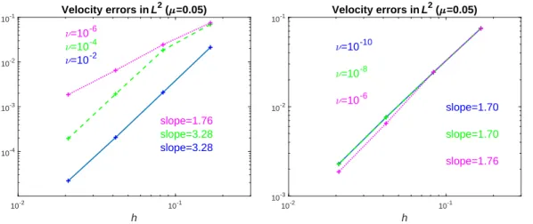
Figure 1: Velocity errors (76) for T = 5 and µ= 0.05. Left, large to moderate viscosity. Right moderate to small viscosity.

We used P2/P1 pair of mixed finite-elements on a regular triangulation with

SW-NE diagonals. We used meshes with N = 6, 12, 24 and 48 subdivisions in each coordinate directions. The value of ∆t was set to ∆t = 0.05 for the coarser mesh, and divided by 8 every timeN was doubled. Repeating the experiments with values of ∆ttwice as large showed hardly any difference in the errors. Furthermore, for ν ≤ 10−6 there was no difference between the results shown here and those obtained by dividing ∆tby four every time N was doubled. All this suggests that in the errors shown in the figures below the dominant part comes from the spatial discretization. In the first three figures we show errors

max

0≤n≤Nku n

h−Ih(un)k0, forN =T /∆t, (76)

where Ih is the standard Lagrange interpolant. The grad-div parameter µ was set

to µ= 0.05, since this was the optimal value (marginally, though) among the few we tried from µ= 0.01 to µ= 10. For the nonlinear term, we used ((2un−un−1)· ∇)un+1 _{instead ofB(u}n_,un+1_{), so that theO(∆t) expected decay of the errors is}

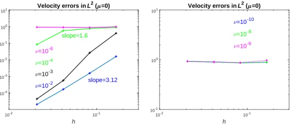
due to the discretization of the time derivative ∂tu. We remark that for µ= 0.05 we did not notice any significant difference between the results presented here and those with B(2un−un−1,un+1). For the case µ = 0 in Fig. 2, though we used

10-2 10-1 h 10-4

10-3 10-2 10-1 100 101

Velocity errors in L2 ( =0)

=10-2 =10-3 =10-4 =10-6

slope=3.12 slope=1.6

10-2 10-1

h 10-1

100 101

Velocity errors in L2 ( =0)

=10-10

=10-8

=10-6

Figure 2: Velocity errors (76) for T = 5 and µ = 0. Left, large to moderate viscosity. Right moderate to small viscosity.

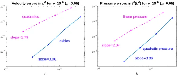
In Fig. 3 for ν = 10−6 and µ= 0.05, we show velocity errors (76) and pressure errors

∆t T /∆t

X

j=1

kpn_h−Ih(pn)k20

1/2

(77)

where Ih is the standard Lagrange interpolant, for mixed pairs quadratic velocity and linear pressure and cubic velocity and cuadratic pressure. As our analysis predicts, orders of convergence are one unit higher for the second pair of elements.

Although our analysis suggests that due to factors µand 1/µon the right-hand side of the error bounds it is advisable to keepµindependent ofh, some researchers find it odd that µ should not depend on h. Results on the left plot in Fig. 4 seem to reinforce that point of view, since takingµ= 0.05h do not significantly alter the velocity errors of µ= 0.05. However, in view of error constantC1 in (26) this may be due to the fact that the second spatial derivatives of the pressure are of moderate size. If we alter the right-hand side f in the Navier-Stokes equations so that the velocity is as in (74) but the pressure is

p(x, y, t) = 10(6 + 4 cos(4t)) sin(2πx) cos(3πy), (78)

the termµ−1_max

0≤t≤Tkp(t)k2_kmakes a significant contribution to the constantC1,

as in can be seen in the right plot on Fig. 4, where the errors when µ = 10h

have a lower rate of decay with h as compared to those of µ = 10 (the value that produced marginally better results from those tried between µ= 1 and µ = 100). Thus, although making µdepend on h may not damage results with respect those of fixed µ in some cases, it may considerably worsen them in some other cases, so that, in accordance with the analysis, it seems to be advisable to takeµindependent of h.

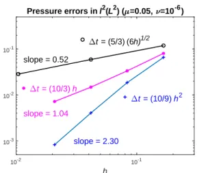
Finally, we check if the time step restriction (63) is sharp in practice or if it is a consequence of the limited techniques of analysis. In Fig. 5 we show the errors (77) when ∆tis taken proportional to h2 toh and toh1/2. Notice that only ∆t=Ch2

10-2 10-1 h 10-4

10-3 10-2 10-1

Velocity errors in L2 for =10-6 ( =0.05)

quadratics

cubics slope=1.78

slope=3.06

10-2 10-1

h 10-4

10-3 10-2 10-1

Pressure errors in l2(L2) for =10-6 ( =0.05)

linear pressure

quadratic pressure slope=2.04

slope=3.06

Figure 3: Velocity errors (76) (left) and pressure errors (77) (right) for quadratic and cubic velocity approximation (linear and quadratic pressure approximation, respectively).

10-2 10-1

h 10-3

10-2 10-1 100

Velocity errors in L2

=0.05 =0.05h

10-2 10-1

h

10-3 10-2 10-1 100

Velocity errors in L2

=10

=10h

Figure 4: Velocity errors (76) for ν = 10−6_{. Left, pressure as in (75). Right, pressure as}

10-2 10-1 h 10-3

10-2 10-1

Pressure errors in l2(L2) ( =0.05, =10-6)

t = (10/9) h2

slope = 2.30

t = (10/3) h

slope = 1.04

t = (5/3) (6h)1/2

slope = 0.52

Figure 5: Pressure errors for ν = 10−6_.

the two finest meshes. It can be seen that errors decay like ∆t in all three cases, suggesting that (63) is not sharp in practice, but rather a limitation imposed by the techniques of analysis.

4.2

Flow past a cylinder

We consider the well-known benchmark problem defined in [46]. The domain is

Ω = (0,2.2)×(0,0.41)/

(x, y)|(x−0.2)2+ (y−0.2)2 ≤0.0025

and the time interval [0,8]. In both vertical sides the velocity is given by

u(0, y) =y(2.2, y) = 6 0.412 sin

πt

8

y(0.41−y)

0

,

while in the rest of the boundary it is set u=0. Also, att= 0, the initial velocity isu=0. The kinematic viscosity is set toν= 10−3 and the forcing term is f =0. It is well-known that around t= 4 a vortex sheet develops behind the cylinder, as it can be seen in Fig. 6 when we show the speed and velocity field for t = 5 tot= 8. The four plots of the velocity fields are plotted in the same scale, and we obtain virtually the same plots as in [35, Fig. 2]

We present errors in maximum values of the drag and lift coefficients cd and cl

respectively, and the difference of the pressure

∆p(t) =p(0.15,0.2, t)−p(0.25,0.2, t)

between the front and the back of the cylinder at t= 8

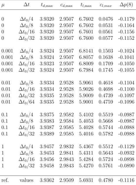
We also computed errors in the timestdandtlwhere the lift and drag coefficients, respectively, attained their maximum values. To compute all these errors, reference values are taken from [35]. Also, following suggestions in [35], we computecdandcl

as

cd(t) =−20 ν(∇u(t),∇vd) +b(u(t),u(t),vd)−(p(t),∇ ·vd)

,

cl(t) =−20 ν(∇u(t),∇vl) +b(u(t),u(t),vl)−(p(t),∇ ·vl)

Figure 7: Coarsest and finest meshes used in Fig. 9.

wherevdandvlare piecewise linear functions vanishing on triangles without vertices

on the circumference c≡(x−0.2)2+ (y−0.2)2 = 0.0025. and taking values vd=

[1,0]T and vl= [0,1]T on those nodes on circumference c.

We computed approximations on a sequence of five meshes the coarsest and finest ones being shown in Fig. 7. The total number of degrees of freedom (dgf) of the approximations to the velocity and pressure on these grids are 2057, 4208, 7709, 16961, 46265, so that they are coarser than those used in [35]. We used quadratic isoparametric elements for the velocity and linear elements for pressure. We present results corresponding toµ= 0 andµ= 0.01. This last value was chosen for producing the best results among those with which we tried on one of the grids, the fourth one from coarser to finer, as it can be seen in Table 1 in Appendix B. For each mesh, decreasing values of ∆t were tried until the first two digits in the computed error no longer changed. The computed quantities on each grid and for every value of ∆t are shown in in Tables 2 and 3 in Appendix B. In the present section, we present some plots corresponding to the smallest values of ∆t for each grid in those tables.

In Fig. 8 we show the evolution of the drag and lift coefficients and of ∆p(t) for

µ= 0.01 in blue and forµ= 0 in magenta. This plots should be compared with [35, Fig. 4]. The reference values (taken from [35]) of the maximum values cd,max of the drag coefficient andcl,max of the lift coefficient are marked with a red asterisk

at time td,max and tl,max, respectively, where they are achieved, according to [35].

We also mark with a red asterisks the reference value for ∆p(8). It can be seen that already for the medium sized grid (dgf=7709) the evolution ofcd here (top left

plot in Fig. 8) is very much alike to that in [35, Fig. 4], that the reference value of cd,max is matched, at least visually, and that the results corresponding to µ= 0

are superimposed to those of µ= 0.01.

For the lift coefficient, however, we see that while the results with µ = 0.01 resemble those in [35, Fig. 4] (specially for the two finest grids, for which the cor-responding results are presented in the second row) this is clearly not the case when µ= 0. Only for the finest grid (second row, right plot) have the results with

µ= 0 a resemblance to those in [35, Fig. 4]. We conclude then that, for the case of the lift coefficient, adding grad-div stabilization does indeed improve accuracy.

0 1 2 3 4 5 6 7 8 time

-0.5 0 0.5 1 1.5 2 2.5 3

Drag coefficient c_d (dgf=7709)

=0.01

=0

0 1 2 3 4 5 6 7 8

time -0.5

0 0.5

Lift coefficient c_l (dgf=7709)

=0.01

=0

0 1 2 3 4 5 6 7 8

time -0.5

0 0.5

Lift coefficient c_l (dgf=16961)

=0.01

=0

0 1 2 3 4 5 6 7 8

time -0.5

0 0.5

Lift coefficient c_l (dgf=46265)

=0.01

=0

0 1 2 3 4 5 6 7 8

time -0.5

0 0.5 1 1.5 2

2.5 Pressure difference p (dgf=7709)

=0.01

=0

7.96 7.97 7.98 7.99 8 8.01 8.02 8.03 8.04

time -0.13

-0.125 -0.12 -0.115 -0.11 -0.105 -0.1

Pressure difference p. Detail

=0, dgf=7709

=0.01, dgf=7709 =0.01, dgf=16961

=0, dgf=16961 exact value at t=8

103 104 degrees of freedom 10-4

10-3 10-2

Relative errors in c

d,max

=0

=0.01

103 104

degrees of freedom 10-2

10-1 100

Relative errors in c

l,max

=0

=0.01

103 104

degrees of freedom 10-3

10-2 10-1

Relative errors in p(8)

=0

=0.01

103 104

degrees of freedom 10-2

10-1

Geometric mean of all five relative errors

=0

=0.01

Figure 9: Flow around a cylinder: relative errors. Bottom right plot shows the geometric mean of relative errors in cd,max,td,max, cl,maxl, tl,max and ∆p(8).

16961 dgf, for which the corresponding results are also shown.

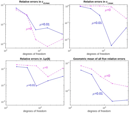
The plots in the bottom row in Fig. 8 suggest that checking the errors with respect reference values may add further information. In Fig. 9 we present the relative errors in the computation of cd,max,cl,maxand ∆p(8). It can be seen adding

grad-div stabilization worsens the accuracy of the drag coefficientcd,max(the easiest coefficient to compute accurately, according to [35]), but improves that of the lift coefficient cl,max (the most difficult one to compute accurately, according to [35])

and ∆p(8). To have an idea of the overall improvement of adding the grad-div term, we show in the last plot in Fig. 9 the geometric mean of the relative errors in five computed quantities, cd,max, cl,max, ∆p(8), td,,max and tl,max. We can see that, on

average, adding the grad-div term improves the overall accuracy in the computation of the five quantities. We notice, however, that as the meshes are refined, the values of the quantities computed with and without the grad-div term seem to get more similar, at least in the case of cd,max and cl,max. This is in agreement with results