Finding the Number of Normal Groups in Model Based Clustering via Constrained Likelihoods

Finding the Number of Normal Groups in

Model-Based Clustering via Constrained

Likelihoods

Andrea Cerioli

Dipart. di Scienze Economiche e Aziendali, Universit`

a di Parma

Luis Angel Garc´ıa-Escudero

Dpto. de Estad´ıstica e I.O. and IMUVA, Universidad de Valladolid

Agust´ın Mayo-Iscar

Dpto. de Estad´ıstica e I.O. and IMUVA, Universidad de Valladolid

and

Marco Riani

Dipart. di Scienze Economiche e Aziendali, Universit`

a di Parma

October 5, 2018

Abstract

Deciding the number of clusters k is one of the most difficult problems in clus-ter analysis. For this purpose, complexity-penalized likelihood approaches have been introduced in model-based clustering, such as the well known BIC and ICL crite-ria. However, the classification/mixture likelihoods considered in these approaches are unbounded without any constraint on the cluster scatter matrices. Constraints also prevent traditional EM and CEM algorithms from being trapped in (spurious) local maxima. Controlling the maximal ratio between the eigenvalues of the scatter matrices to be smaller than a fixed constant c≥1 is a sensible idea for setting such constraints. A new penalized likelihood criterion which takes into account the higher model complexity that a higher value ofcentails, is proposed. Based on this criterion, a novel and fully automated procedure, leading to a small ranked list of optimal (k, c) couples is provided. A new plot called “car-bike” which provides a concise summary of the solutions is introduced. The performance of the procedure is assessed both in empirical examples and through a simulation study as a function of cluster overlap. Supplemental materials for the article are available online.

1

Introduction

Cluster analysis is the art of clustering a data set into k groups of similar individuals. One

of the main difficulties (and one of the most widely addressed problems) when using cluster

analysis methods is how to decide the number of clusters k to be found. Sometimes k is

known in advance because of the application in mind, but most of the timesk is completely

unknown and we want the data set itself to suggest a “sensible” number of groups. Several

approaches for determining the number of clusters can be found in the literature (see, e.g.,

Milligan and Cooper, 1985; Rousseeuw, 1987; Tibshirani et al., 2001, among many others).

In this work we tackle the problem from a model-based perspective, with a normality

assumption for the cluster components. Let x1, ..., xn be the observations in Rp to be

clustered and let ϕ(·;µ,Σ) denote the p.d.f. of thep-variate normal distribution with mean

µ and covariance matrix Σ. In model based clustering, there are two distinct approaches

depending on whether the mixture or the classification likelihood function is used.

The first approach is based on maximization of the mixture log-likelihood (MIX)

Lk(θ) = n

∑

i=1 log

[ _k ∑

j=1

pjϕ(xi;mj, Sj)

]

,

where θ = (p1, ..., pk, m1, ..., mk, S1, ..., Sk) is the set of parameters satisfying pj ≥ 0 and

∑k

j=1pj = 1, mj ∈ Rp and Sj a p.s.d. symmetric p ×p matrix. The optimal set of

parameters based on this likelihood is

b

θMixt,k = arg max

θ Lk(θ). (1)

Once θbMixt,k = (pb1, ...,pbk,mb1, ...,mbk,Sb1, ...,Sbk) is obtained, the observations in the sample

are divided into k clusters by using posterior probabilities. That is, observation xi is

assigned to cluster j if j = arg maxlpblϕ(xi;mbl,Sbl).

The second approach is based on maximization of the classification log-likelihood (CLA)

CLk(θ) = n

∑

i=1

k

∑

j=1

zij(θ) log

(

pjϕ(xi;mj, Sj)

)

,

where θ = (p1, ..., pk, m1, ..., mk, S1, ..., Sj) and

zij(θ) =

  

1 if j = arg maxlplϕ(xi;ml, Sl)

In this case, the optimal set of parameters is

b

θClas,k = arg max

θ CLk(θ) (2)

and observation xi is now classified into clusterj if zij(bθClas,k) = 1.

Based on the two different likelihood approaches (1) and (2), some proposals exist that

lead to sensible ways for choosing the number of clusters. The basic idea is to maximize

over k some complexity-penalized versions of these two likelihoods. Specifically, it is a

common practice to add penalty terms depending on the number of free parameters in the

model. Following this idea and taking the usual log-likelihood transformation, we envisage

three possibilities:

MIX-MIX : kopt = arg min

k

{

−2Lk(bθMixt,k) +vk

}

MIX-CLA : kopt = arg min

k

{

−2CLk(θbMixt,k) +vk

}

CLA-CLA : kopt = arg min

k

{

−2CLk(θbClas,k) +vk

}

wherevk is the penalty term counting the number of free parameters. This term is typically

chosen as vk = (kp+k−1 +k(p+ 1)p/2) log(n), if no particular constraints are posed on

the scatter matrices S1, ..., Sk. In our notation, “MIX-MIX” corresponds to the use of the

Bayesian Information Criterion (BIC) (see, e.g., Fraley and Raftery (2002); Fraley et al.

(2017)), while “MIX-CLA” corresponds to the use of the Integrated Complete Likelihood

(ICL) method proposed by Biernacki et al. (2000). The rationale behind the ICL criterion

is that “mixture modeling” is a different problem from “clustering” and, thus, the number

of groups obtained as a solution to these problems may not be the same. “CLA-CLA” is

instead rooted in the crisp clustering framework of (2) and, to our knowledge, a novelty

of this paper. The consideration of weights pj in classification likelihoods, as in CLk(θ),

goes back to Symons (1981). Bryant (1991) mentioned the possible interest in classification

likelihoods with weights to choose the number of groups in clustering, but without adding

an extra penalty term for model complexity. It is important to note that the maximization

of the classification and mixture likelihoods are both ill-posed problems because of their

unboundedness without any constraint on the scatter matrices of the fitted normal

for all the eigenvalues of the scatter matrices. In addition, this eigenvalue ratio constraint

is also useful to prevent traditional EM algorithms from being trapped in (non-interesting)

spurious local maxima. This type of constraint depends on a fixed constant c in such a

way that smallercvalues favor cluster sphericity and homoscedasticity among groups. The

use of penalized likelihood criteria under constraints, where the penalty term takes into

account the higher model complexity entailed by a higher c value, suggest new criteria

that will be denoted as MIXc-MIX, MIXc-CLA and CLAc-CLA. Once the user is able to

specify the type of cluster of interest through the specification of the constant c, these new

criteria can be used to choose the number of clustersk. However, there are cases when that

specification is not at all straightforward for the user. In those cases, as one of the main

contributions of this work, we propose a fully automated procedure producing a small and

ranked list of optimal (k, c). All these “best ranked” solutions can be further examined, by

applying validation tools in cluster analysis or taking into account the final user purposes,

in order to choose the one that better fits the aims of analysis.

The outline of our work is as follows. The need for constraints in model-based clustering

is reviewed in Section 2 where the maximal eigenvalue ratio constraints are also presented.

Section 3 shows how well-known criteria can be adapted in this constrained setting in such

a way that a “sensible” number of clusters/components can be found when the constant c

is fixed in advance. Section 4 addresses the important problem of choosing simultaneously

bothkandc. Section 5 presents an automated procedure that returns a ranked small list of

“optimal” cluster partitions and introduces a new plot which provides a concise summary

of the best solutions. This procedure is illustrated in practice with both simulated and

well-known real data sets. Section 7 describes a simulation study that shows the effectiveness of

the proposed methodology under general settings. Finally, Section 8 concludes and provides

some open lines for future research.

2

Constrained clustering approaches

The need for constraints on the scatter matrices arises because both (1) and (2) are

un-bounded (just takeµ1 =x1and|Σ1| →0). Therefore, the associated maximization becomes

appro-priate constraints often leads the algorithms proposed for numerical maximization of (1)

and (2) to be trapped in local maxima of the likelihood, associated to the detection of

non-interesting “spurious solutions” (see, e.g., McLachlan and Peel, 2000).

The lack of boundedness of (1) and (2) is often circumvented by resorting to

“appropri-ate” initializations of the EM or CEM algorithms. Although this strategy is appealing, we

note that, in this case, we would not be exactly trying to maximize the target functions in

(1) and (2). In fact, it is known (see, e.g., Maitra (2009)) that the result of applying EM

and CEM algorithms is strongly dependent on the chosen initialization, which may severely

affect the value of the associated likelihoods and, consequently, the choice of k provided

by MIX-MIX, MIX-CLA and CLA-CLA. For instance, we may have trouble with

elon-gated parallel clusters when using thek-means method, or we can be affected by undesired

“chaining effects” when considering single-linkage hierarchical clustering.

Furthermore, it is important to note that cluster analysis is also not a well-defined

problem from an applied viewpoint. There is nowadays a wide consensus about the fact

that clustering techniques should always depend on the final data-analysis purpose, so that

different goals require the use of different clustering approaches. Figure 1 in Hennig and

Liao (2013) shows a toy example – to which we will return in Section 5.2.2 – with a data set

obtained as a realization of a mixture of three well-separated bivariate normal components.

Any clustering approach purely based on mixture modeling would determine the existence

of three clusters. However, a “social stratification” framework, such as that exemplified

in Hennig and Liao (2013), would clearly require the determination of more than three

clusters. Similar conclusions could also hold in other important application fields, such as

market research, where the construction of relevant clusters must often be coupled with

subject matter aims. We thus argue that clustering should not be seen as a fully automatic

task providing just one single solution and that the user always has to play an active role

in it. The consideration of appropriate constraints onθ, when maximizing (1) and (2), may

allow the user to specify somehow the partitions of actual interest. This is another major

reason that motivates our interest in introducing constraints in cluster analysis.

Some of the available solutions are based on imposing constraints on the elements of

matrices allow us to obtain parsimonious variants of the unconstrained normal mixture

model in such a way that (most of them) successfully serve to avoid spurious maximizers and

convert the maximization of the likelihood into a well-defined problem. More details of these

parsimonious parameterizations can be seen in Banfield and Raftery (1993) and Celeux and

Govaert (1995). The resulting parameterizations can be easily addressed with the criteria

described in Section 1 just by taking into account the number of free parameters. Another

possibility, going back to Hathaway (1985), has been proposed and explored in Ingrassia and

Rocci (2007) and Garc´ıa-Escudero et al. (2008, 2015). The approach is based on controlling

the maximal ratio between the eigenvalues of the cluster scatter matrices. This implies

maximizing the likelihoods (1) and (2), withθ ∈Θcwhere Θc =

{

p1, ..., pk with

∑k

j=1pj =

1;m1, ..., mk inRp;S1, ..., Sk p.s.d. matrices with λl(Sj) ≤ cλq(Sh) for every j, l, h, q

}

. In

the above, {λl(S)}p_l=1 stands for the set of eigenvalues for the scatter matrix S. Note that

through the constant c≥1 we are simultaneously controlling discrepancies from sphericity

and differences among cluster scatters. The parameter c can be interpreted as the square

root of the maximal ratio among the lengths of the equidensity ellipsoids defined by the

ϕ(·;mj, Sj) normal densities. Accordingly, we can define two constrained problems: the

constrained mixture likelihood maximization (MIXc)

b

θc_Mixt,k = arg max

θ∈Θc

Lk(θ), (3)

and the constrained classification likelihood maximization (CLAc)

b

θ_Clasc _,k = arg max

θ∈Θc

CLk(θ). (4)

The algorithms in Fritz et al. (2013) and in Garc´ıa-Escudero et al. (2014) can

respec-tively be used to approximately solve these constrained maximizations. In these algorithms

an eigenvalue truncation procedure is applied to enforce the eigenvalues ratio constraint

in the EM and CEM steps. These algorithms always increase the likelihood functions

throughout constrained EM and constrained CEM steps and so serve to find local maxima

of the likelihood under the required constraints. Several random initializations are used

when trying to find the global constrained maximum. Finally, an alternative approach can

be found in Fraley and Raftery (2007) where semi-informative priors are placed on the

eigenvalues of the covariance matrices. This results in a posterior mode, subsequently used

3

Penalized likelihoods in constrained clustering

We now define the MIXc-MIX, MIXc-CLA and CLAc-CLA criteria for choosing the number

of clusters when following the constrained maximization targets (3) and (4) for a fixed

constant c≥1. This requires a modification of the “penalty term”, which should take into

account the higher model complexity that a higher c value entails. We propose the use of

a penalty term v_kc defined as

v_kc =

   

kp+k−1 +k

p(p−1) 2

| {z }

rotation par.

+ (kp−1)

(

1− 1

c

)

+ 1

| {z }

eigenvalue par.

   

logn. (5)

Here we have distinguished the parameters related to orthogonal rotations of the scatter

matrices – which are not affected by constraints – and those related to the eigenvalues.

In the most constrained case (c = 1), all the eigenvalues are equal, i.e. there is only one

free extra parameter related to the eigenvalues. On the other hand, we recoverkp(p+ 1)/2

free parameters for the scatter matrices when we approximate the fully unconstrained case

c→ ∞. A justification for this “soft” transition between the two extreme cases is as follows.

If no constraints are posed on the whole set of eigenvalues of the scatter matrices, say

λ1, ..., λD (withD=k×p), then we have the reference setA={(λ1, ..., λD) : 0≤λl}.In the

constrained case, we consider the set B = {(λ1, ..., λD) : 0 ≤ λl ≤ cλq for every l ̸=q}. A

very simple idea is to consider the relative volume of setBwith respect toAas a complexity

measure. Of course, this ratio between volumes is not well-defined since neither A nor B

are bounded sets. However, we can take into account that A =∪_t≥0At and B =

∪

t≥0Bt, with At and Bt being sets defined as in the statement of Theorem 3.1.

Theorem 3.1 Let At = {(λ1, ..., λD) : 0 ≤ λl ≤ t} and Bt = {(λ1, ..., λD) : 0 ≤ λl ≤

t; λl≤cλq for every l̸=q}. Then

Vol(Bt)

Vol(At)

=

(

1− 1

c

)D−1

.

The proof and a graphical illustration are left to the “online supplementary material”.

Theorem 3.1 is implicitly applied in our definition of the penalty term (5) by seeing that

are “relatively” weighted by the multiplicative factor (1−1_c). By considering the modified

penalty termvc

k, we have the following three new criteria for choosing the number of clusters

depending on the maximal eigenvalue ratio c:

MIXc-MIX :kopt,MM(c) = arg min

k

{

−2Lk(θbMixt,kc ) +v

c k

}

:= arg min

k FMM(k, c)

MIXc-CLA :kopt,MC(c) = arg min

k

{

−2CLk(θbcMixt,k) +vck

}

:= arg min

k FMC(k, c)

CLAc-CLA :kopt,CC(c) = arg min

k

{

−2CLk(θbcClas,k) +v

c k

}

:= arg min

k FCC(k, c).

Unlike the standard MIX-MIX, MIX-CLA and CLA-CLA criteria, here the use of our

constrained proposals provides well-defined problems where the corresponding target

func-tions Fm(k, c), m =MM, MC or CC, are bounded for a fixed 1 ≤ c < ∞. Moreover,

spurious solutions are avoided provided that the supplied value cis not very large

(Garc´ıa-Escudero et al., 2015). The specification ofc may be seen as a sensible way for the user to

declare the maximum allowed difference on cluster scatters that he/she is willing to admit.

This choice then depends on the final clustering purpose in mind. For instance, the social

stratification problem in Hennig and Liao (2013) would require the user to specify a value

of cclose to 1. This implies the search of almost spherical clusters with similar scatters or,

analogously, the use of the Euclidean distance for clustering. Other problems would require

larger values of c, and so the detection of less restricted clusters. Once the value of c has

been fixed, the determination of kopt,m(c) is done by minimizing the previously introduced

criteria with respect to k for a given methodm where m=MM, MC or CC. It should also

be noted that this approach is not affine equivariant due to the lack of equivariance of the

chosen constraints. Therefore, standardizing the variables may be needed if, for instance,

very different scales are involved.

To illustrate how the methodology can be applied, let us consider a simulated data

set of size n = 100 and dimension p = 2 from a k = 3 component mixture obtained

by applying the MixSim method of Maitra and Melnykov (2010), as extended by Riani

data set has been generated by imposing an average cluster overlap (defined as a sum of

pairwise misclassification probabilities) equal to 0.04 and a maximum eigenvalue ratio for

the scatters matrices equal to 5. Given two clusters j and l (j ̸=l = 1, ..., k), indexed by

ϕ(x;mj, Sj) andϕ(x;ml, Sl), with probabilities of occurrencepj andpl, theoverlapbetween

groups j and l is defined as sum of the two misclassification probabilities wjl =wj|l+wl|j

where wj|l = P r[plϕ(x;ml, Sl) < pjϕ(x;mj, Sj)]. The average overlap is the sum of the

off-diagonal elements of the matrix of the misclassification probabilities wj|l divided by

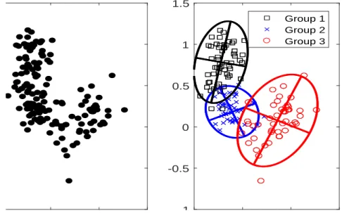
k(k−1)/2. Figure 1 shows two scatter plots of this simulated data set, without and with

the “true” assignments labels. It is not perfectly clear by visual inspection, at least looking

at the graph in the left panel, whether there are two or three clusters.

0 0.5 1 1.5

-1 -0.5 0 0.5 1 1.5

0 0.5 1 1.5

-1 -0.5 0 0.5 1 1.5

Group 1 Group 2 Group 3

Figure 1: Simulated bivariate data set. The panel on the right shows the data set with the

“true” labels and tolerance ellipsoids summarizing the three normal components.

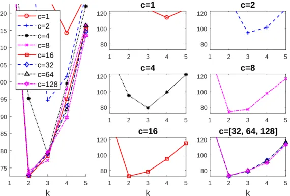
Figure 2 shows the curves of our objective function that are obtained by monitoring

FCC(k, c) when c ranges over the interval [1,128] and k (x axis) goes from 1 to 5. The

large left panel shows all the 8 trajectories of FCC(k, c) that are obtained by considering

c ={20,21,22, ...,27}. The value of c for the lowest curve at each k is shown in the table

below the caption of the Figure. For instance, whenk = 2 the lowest value is forc= 16; for

k = 3 the lowest value is for c= 8; etc.. Given that the eight trajectories strongly overlap,

of cwe have considered (c= 1,2,4,8,16). The trajectories for the 3 largest values ofc are

very similar and, thus, they are all reported in the same final right panel.

1 2 3 4 5

k 75 80 85 90 95 100 105 110 115 120 _c=1 c=2 c=4 c=8 c=16 c=32 c=64 c=128

1 2 3 4 5

80 100 120

c=1

1 2 3 4 5

80 100 120

c=2

1 2 3 4 5

80 100 120

c=4

1 2 3 4 5

80 100 120

c=8

1 2 3 4 5

k 80

100 120

c=16

1 2 3 4 5

k 80

100 120

c=[32, 64, 128]

Figure 2: Analysis of the modified constained criteria when using the CLAc-CLA approach

for the data set shown in Figure 1.

By using the curves plotted in Figure 2, we can see that the optimal values for the

number of clusters are, for instance, kopt,CC(2) = 3 (i.e., when c = 2) or kopt,CC(16) = 2

(i.e., when c = 16). We thus obtain k = 3, which corresponds to the true number of

components, when we are interested in neither very spherical nor homoscedastic clusters,

but we find k = 2 clusters when we allow for more elongated group structures. The latter

also provides a sensible cluster partition, from a clustering point of view, since Group 1

and Group 2 (right panel of Figure 1) may be seen as being part of the same cluster if only

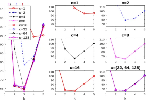
the left panel of Figure 1 is visualized. Similar plots are given in Figure 3 when FMM(k, c)

is monitored. We can see that the use of an objective function more focused on “mixture

modeling”, such as MIXc-MIX, always suggests kopt,MM(c) = 3 (i.e., the true number of

mixture components) for every value of c > 1 tried. A higher number of groups is only

1 2 3 4 5 k 65 70 75 80 85 90 95 100 105 110 c=1 c=2 c=4 c=8 c=16 c=32 c=64 c=128

1 2 3 4 5

70 80 90 100 110 c=1

1 2 3 4 5

70 80 90 100 110 c=2

1 2 3 4 5

70 80 90 100 110 c=4

1 2 3 4 5

70 80 90 100 110 c=8

1 2 3 4 5

k 70 80 90 100 110 c=16

1 2 3 4 5

k 70 80 90 100 110

c=[32, 64, 128]

Figure 3: As Figure 2, but now for MIXc-MIX.

4

Simultaneous choice of

k

and

c

Alternatively, we may know the number of groups k due to some economic, physical or

operational reason, when our aim is that of obtaining a sensible value for c. Notice that

in this case the user does not want to impose any particular structure on the clusters to

be detected. This goal can be achieved by using the same penalized criteria as before, but

now minimizing over c. Therefore, if k is assumed to be known, we take

copt,m(k) = arg min

c Fm(k, c), for m= MM, MC and CC,

as our choice for the optimal value of c. This information is included in the “online

sup-plementary material” for the data set shown in Figure 1.

In practice the most interesting case is when both the proper number of clustersk and

the constraining factor c are unknown. We have argued before that a fully unsupervised

choice of both parameters, depending only on the data set at hand, is very likely to be out of

reach for most applications. Nevertheless, it would be helpful if we were able to reduce the

in order to find more easily the pair that best fits the user’s main purpose in clustering.

One might think that direct study of the functionals (k, c) 7→ Fm(k, c), for m =

MM, MC and CC, would provide valuable information about how to choose

simultane-ouslyk and c. Contour plots that summarize the resulting monitoring process for the data

set shown in Figure 1 are in the “online supplementary material”. Our experience is that

these contour plots are not easily interpreted. Additionally, there are partitions obtained

with different (k, c) parameters that correspond to essentially the same substantial groups,

or that simply differ because of the inclusion of extra (non-interesting) spurious clusters.

5

Automated selection of a list of “sensible” solutions

5.1

Methodology

In this section, we offer a fully automated procedure that leads to a small and ranked list

of “optimal” choices for the pair (k, c). The proposed methodology, based on our three

constrained clustering criteria, relies on analysis of the stability of the cluster partitions

through the Adjusted Rand Index (ARI). The ARI is a measure of the similarity between

two data clusterings after “adjusting for chance”. The adjusted Rand index is thus ensured

to have a value close to 0 for random labeling independently of the number of clusters and

samples and exactly 1 when the clusterings are identical (up to a permutation). Specifically,

the procedure first detects a list withL “plausible” partitions. Such “plausible” partitions

may include some partitions that are essentially the same as others already detected,

be-cause spurious clusters made up with few almost collinear or very concentrated data points

are found. In a second step, the partitions including spurious clusters are discarded and

we end up with a (typically very) reduced and ranked list with T “optimal” partitions.

Given a pair (k, c), let P(k, c) denote the partition into k subsets which is obtained by

solving the problem (3) or (4), with the given k and c and one of the suggested methods

m = MM, MC and CC. Let ARI(A,B) denote the ARI between partitions A and B. We

consider that two partitions A and B are “essentially the same” when ARI(A,B)≥ε, for

a fixed thresholdε. Clearly, the higher the value of the threshold the greater is the number

Let us consider the sequencek = 1, ..., K, where K is the maximal number of clusters,

and a sequence c = c1, ..., cC of C possible constraint values. For instance, the sequence

of powers of 2, c1 = 20, c2 = 21, ..., cC = 2C−1 is recommended because it enables us to

consider a sharp grid of values close to 1. By using this notation, the proposed automated

procedure may be described as follows:

1. Obtain the list of “plausible” solutions:

1.1 Initialize: Start withK×Cpossible (k, c) pairs to be explored. LetE0 ={(k, c) :

k = 1, ..., K and c=c1, ..., cC}.

1.2 Iterate: IfEl−1 is the set of pairs (k, c) not already explored at stagel−1, then:

1.2.1 Obtain (kl

∗, cl∗) = arg min(k,c)∈El−1Fm(k, c).

1.2.2 Remove all of the cluster partitions (k, c)∈ El−1 withk =k_∗l and values of c

which are adjacent to cl

∗, and such that they are very “similar” to partition

P(kl_∗, cl_∗) for the given threshold value ε, in the sense that

ARI(P(k, c),P(k_∗l, cl_∗))≥ε. (6)

TakeEl as the setEl−1 after removing the pairs yielding “similar” partitions.

1.3 Finalize: The iterative procedure ends when EL = ∅ (or when L is a positive

prefixed integer number) and it returns {(k1

∗, c1∗),(k2∗, c∗2), ...,(k∗L, cL∗)} as a list

with L “feasible” parameters combinations.

2. Obtain the list of “optimal” solutions:

2.1 Initialize: Start from I0 ={1, ..., L} and the L×L matrix (dr,s)r,s=1,...,L, where

dr,s= ARI(P(kr_∗, cr_∗),P(k_∗s, cs_∗).),

2.2 Iterate: Given It−1 the non discarded “plausible” solutions at stage t−1:

2.2.1 Take (k_optt , ct_opt) = (klt

∗, cl∗t) where lt is the t-th element of It−1 (where the indexes inIt−1 are sorted from lowest to highest).

2.2.2 Discard “spurious” solutions (i.e., those that are similar to the already

2.3 Finalize: The iterative procedure ends when IT =∅. It returns

{(k_opt1 , c1_opt),(k_opt2 , c2_opt), ...,(k_optT , cT_opt)}

as the “optimal” pairs.

To simplify notation, we have deleted the subscriptmfor the criterion used (i.e., (kt

opt, ctopt) should be (kt

opt,m, ctopt,m) form= MM, MC and CC). Additionally, the complete automated

procedure is hereinafter referred to autMIXMIX,autMIXCLA and autCLACLA.

For each “optimal” pair (kt

opt, ctopt), it is also informative to take into account the so-called “best interval” Bt defined as

Bt ={c:Fm(koptt , c

t

opt)≤Fm(ktopt, c)}, (7)

and the so-called “stable interval” defined as

St ={c: ARI(P(ktopt, c),P(k

t

opt, c

t

opt))≥ε}. (8)

A large interval Bt means that the number of clusterskoptt is “optimal”, in the sense of (7),

for a wide range ofc values. A large intervalSt means that the solution is “stable”, in the

sense of (8), because it does not essentially change when moving c in that interval.

5.2

Examples

Three examples have been included in the text to exemplify the performance of the proposed

automated procedure. The first has to do with its application to the previously simulated

data set and the second one considers a “toy example” which serves to illustrate how

different cluster partitions may be needed depending on the final clustering purposes. The

third example is based on a more complex “oil data set” withp= 8 variables and a possible

larger number of clusters k. The “online supplementary material” includes an additional

example when the methodology is applied for the classical and well-known “Iris data set”.

5.2.1 Application to simulated data

We have applied the proposed automated procedure with an ARI to the simulated data set

reproduce the analysis displayed in this section can be seen in the “online supplementary

material”. These tables contains the values of CLAc-CLA for all (k, c) pairs and we find

the threshold given in equation (6) considering the matrix which contains the ARI indexes

for two consecutive values of c given k. The first table there shows that (as anticipated

in the previous section) the best value of k is 2 and the second best value of k is 3. The

second table there, on the other hand, shows that for k = 2 (overall best solution) there

is essentially just one solution in the range c [2,128] (the values of ARI in this interval

are all greater than 0.8). For k = 3 (second overall best solution) the solution is stable in

the intervalc [1,128] with many solutions giving exactly the same partition. The situation

seems to be more complex fork = 4 where in the intervalc[16,128] we virtually obtain the

same solution. The ARI index between c= 8 and c= 16 when k = 4 is 0.71 and suggests

a moderate change in the classification, while the one between c= 4 and c= 8 goes down

to 0.57. Finally, the solutions in the interval c [1,4] seem homogeneous. Our procedure

combines in a fully automatic way the information in the two previous tables. The analysis

of the the values of CLAc-CLA for all (k, c) pairs shows that the first best solution is for

k = 2 andc= 16 and that this solution remains the best in the intervalc[8,128] and (if we

consider a threshold of ARI equal to 0.8) we find that this solution is stable in the interval

c[2,128]. In order to find the second solution, we remove from the table with all the values

of CLAc-CLA those (k, c) pairs in which the first solution was stable and check for the new

minimum. The joint examination of the two tables, shows that the second solution takes

place when k = 3, and c = 8, and that this solution is best and stable in the interval c

[4,128] and that is stable in the interval c [1,128]. Given that the ARI index between the

second solution (k = 3 and c= 8) and the first one (k = 2 and c= 16) is 0.38 (below the

prefixed threshold of 0.8 we consider the second solution as non spurious). The procedure

goes on until we find the the first (say) three or four non spurious solutions.

The corresponding four best-ranked solutions are shown in Figure 4. We see that we

recover the true number of clusters k2_opt,CC = 3 in the second solution. The solution with

k1

opt,CC = 2 makes perfect sense from the “pure” clustering point of view adopted by the

CLAc-CLA criterion and, thus, it is the first offered partition. The homoscedastic c = 1

solution is shown as the ninth one and it proposes k9

0 0.5 1 1.5 -1

-0.5 0 0.5 1

1.5 Solution 1: k=2 c=16

Best for c=[8-128] Stable for c=[2-128]

0 0.5 1 1.5

-1 -0.5 0 0.5 1

1.5 Solution 2: k=3 c=8

Best for c=[4-128] Stable for c=[1-128]

0 0.5 1 1.5

-1 -0.5 0 0.5 1

1.5 Solution 4: k=4 c=8

Best for c=[8-8] Stable for c=[8-8]

0 0.5 1 1.5

-1 -0.5 0 0.5 1

1.5 Solution 9: k=5 c=1

Best for c=[1-1] Stable for c=[1-1]

Figure 4: The T = 4 best-ranked partitions when using theautCLACLAprocedure for the

simulated data set displayed in Figure 1.

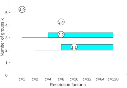
In order to provide a concise summary of the non spurious solutions found and in order

to better distinguish the most relevant solutions from those which are local, we propose a

new graphical display which we call “car-bike”. This plot shows on the horizontal axis the

value of cand on the vertical axis the value ofk. For each solution we draw a rectangle for

the interval of values for which the solution is best and stable and a horizontal line which

departs from the rectangle for the values of cin which the solution is only stable. Finally,

for the best value of c associated to the solution, we show a circle with two numbers,

the first number indicates the ranked solution among those which are not spurious and

the second one the ranked number including the spurious solutions. This plot has been

baptized “car-bike”, because the first best ranked solutions (in general 2 or 3) are generally

best and stable for a large number of values ofcand therefore will have large rectangles. In

addition, these solutions are likely to be stable for additional values of cand therefore are

Finally, local minor solutions (which are associated with particular values of c and k) do

not generally present rectangles or lines and are shown with circles (from here the name

“bikes”). Figure 5 shows the car-bike plot coming from the autCLACLA procedure. This

plot shows that there are two main solutions (“cars”) one with 2 groups and the second

with 3 groups. In this case, the two cars are station wagons because the horizontal line just

departs from the left side of the rectangles. The other two non-spurious solutions (“bikes”)

are for k = 4 and c= 8, and k = 5 and c= 1. An additional bonus of this new graphical

representation is that it allows us to immediately spot the area where the best values of c

lie. If we examine the car-bike plot from a vertical perspective we can see that the optimal

values of c are concentrated in the zone between c= 8 and c = 16. In the car-bike plot,

the height of the rectangles can be made proportional to the order of the ranked solution.

Using this criterion the height of the rectangle of say solution 3 out of 8 is (8−3)/8-th

that of the first. Careful examination of Figure 5 reveals that the height of the rectangle

for the second best ranked solution is slightly smaller than that of the first one.

c=1 c=2 c=4 c=8 c=16 c=32 c=64 c=128

Restriction factor c

0 1 2 3 4 5

Number of groups k

1,1 2,2 3,4 4,9

Figure 5: The “car-bike” plot when using using the autCLACLA procedure for the

simu-lated data set displayed in Figure 1.

A figure showing the first 4 discarded “spurious” solutions for the simulated data set can

be found in the “online supplementary material”. We can see there that these discarded

ob-servations or correspond to solutions close to one already detected “optimal” partition.

A referee suggested us to comment on the choice of the threshold of the ARI index. Our

experience is that the value of the threshold is important just to highlight/hide the local

solutions “bikes”, but plays no rule in the detection of the main solutions (“cars”). In the

example above, we have used a threshold of the Rand index equal to 0.8. If we consider

a threshold of 0.7 the only modification concerns the third non spurious solution (bike

associated withk = 4 andc= 8) which disappears because the third solution (c= 128 and

k = 4 which is spurious and therefore is not pictured in the plot) with the new threshold is

considered stable in the interval c[8,128] (as seen in the “online supplementary material”).

Figure 6 shows the ranked set of “optimal” solutions when using the autMIXMIX

procedure. Notice that, from a mixture modeling point of view, we obtain the correct

number of components (k1

opt,MM = 3) in the first position. This result agrees with the

well known fact that mixture modeling is better suited to address cluster overlap than

“pure” clustering, which instead ideally assumes well-separated clusters. The car-bike plot

(not given here for lack of space) for autMIXMIX shows two big cars and and some bikes

scattered around showing once again the presence of just two relevant solutions.

5.2.2 Application to Hennig and Liao’s type of data

Section 5 in Hennig and Liao (2013) includes a toy example to illustrate that there are

cases “where a mixture model is true and most people may have a natural intuition about

the true clusters” but these clusters “are not necessarily the clusters that a researcher is

interested in”. In the spirit of that toy example, we consider the simulated data set shown

in Figure 7. This data set corresponds to a realization of a mixture of three well-separated

bivariate normal components. Without knowledge of the underlying substantive problem,

one would then agree that k = 3 is a sensible choice for k. However, let us assume (as

Hennig and Liao did) that we are facing a social stratification clustering problem and that

the two variables are, for instance, an income and a status indicator. By choosingk = 3 and

very unrestricted scatter matrices, one cluster would contain both the poorest people with

lowest status and the richest people with the highest status. Therefore, in this particular

0 0.5 1 1.5 -1

-0.5 0 0.5 1

1.5 Solution 1: k=3 c=8

Best for c=[4-128] Stable for c=[1-128]

0 0.5 1 1.5

-1 -0.5 0 0.5 1

1.5 Solution 2: k=2 c=16

Best for c=[8-128] Stable for c=[4-128]

0 0.5 1 1.5

-1 -0.5 0 0.5 1

1.5 Solution 4: k=5 c=1

Best for c=[1-1] Stable for c=[1-32]

0 0.5 1 1.5

-1 -0.5 0 0.5 1

1.5 Solution 6: k=2 c=2

Best for c=[1-2] Stable for c=[1-2]

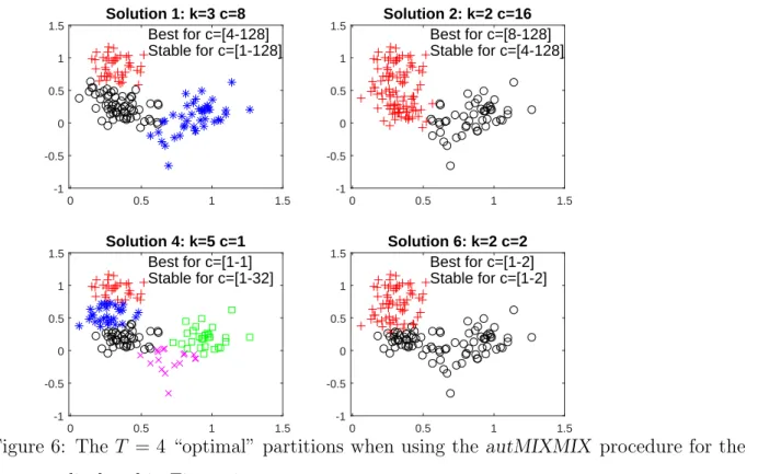
Figure 6: The T = 4 “optimal” partitions when using the autMIXMIX procedure for the

data set displayed in Figure 1.

Figure 7 shows T = 4 “optimal” solutions when using the autMIXMIX procedure. We

can see that the best-ranked partition is exactly the one which discovers the 3 bivariate

normal components. The second and third best ranked partitions offer the user a more

sensible clustering partition for that particular “social stratification” problem. The fourth

best ranked solution offers a very peculiar partition where the two more concentrated

normal components are surprisingly joined together. However, this more “exotic” solution

just appears after the more “sensible” ones. In any case, we think that it is useful to reduce

all the possible pairs (k, c) to such a type of small lists of best-ranked partitions, where the

user can hopefully choose the one that better fits his/her clustering purposes. The car-bike

plot for this data set is presented in the “online supplementary material”.

5.2.3 Olive oil data set

In the previous examples we have seen how our methodology works in the presence of a

0 5 10 15 20 0

5 10 15 20

25 Solution 1: k=3 c=32

Best for c=[32-128] Stable for c=[4-128]

0 5 10 15 20

0 5 10 15 20

25 Solution 3: k=4 c=16

Best for c=[16-16] Stable for c=[1-16]

0 5 10 15 20

0 5 10 15 20

25 Solution 5: k=5 c=16

Best for c=[1-16] Stable for c=[1-16]

0 5 10 15 20

0 5 10 15 20

25 Solution 6: k=2 c=64

Best for c=[16-128] Stable for c=[16-128]

Figure 7: The T = 4 best-ranked partitions when using the autMIXMIX for a data set

similar to that in Hennig and Liao (2013).

and complex dataset which contains several ‘possibly’ overlapping groups.

The “olive oil” data set (Forina et al., 1983) contains p = 8 chemical measurements

on the acid components of n = 572 olive oil specimen produced in various regions in

Italy: (1) North Apulia, (2) Calabria, (3) South Apulia, (4) Sicily, (5) Inland Sardinia,

(6) Costal Sardinia, (7) East Liguria, (8) West Liguria, and (9) Umbria. This data set is

available, for instance, from the pgmm package at CRAN (McNicholas et al., 2015). We

standardize these variables and apply the autMIXMIX criterion with a maximal number

of clusters K = 12 and tentative constraining factors c = 1,2,4, ...,128. The three best

ranked solutions obtained are (c = 128, k = 6), (c = 128, k = 7) and (c = 128, k = 5).

The use of the mclust package (Fraley and Raftery, 2002; Fraley et al., 2017) returns the

following three best ranked models: (VVV, k = 5), (VVV, k = 9) and (VVV, k = 8)

which are obtained by using the BIC criterion. “VVV” stands for ellipsoidal and varying

volume, shape, and orientations. This is in concordance with the choicec= 128, i.e. scatter

Table 1: ARI values of the 3 best ranked solutions with respect to the true regions in the

“Olive oil” dataset. The proposed models appear within parenthesis.

ARI values

First Second Third

autMIXMIX 0.8060 (c= 128,k = 6) 0.8468 (c= 128, k = 7) 0.7441 (c= 128,k = 5)

mclust 0.7763 (VVV,k = 5) 0.6258 (VVV,k = 9) 0.6601 (VVV,k= 8)

best ranked solutions with respect to the true classification in the 9 regions.

In this case the three best partitions returned by autMIXCLA and autCLACLA are

essentially the same (and in the same order) in this case.

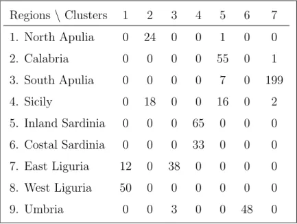
Table 2 shows the confusion matrix for the second best solution (that with ARI value

0.8468). We can see the original oil production regions are quite well recovered in this

suggested cluster partition. The only regions that we are not able to disentangle are regions

2 and 4 (Calabria and Sicily) and regions 5 and 6 (inland and costal Sardinia). A thorough

examination of the scatter plot matrix reveals that oils from regions 2 and 4 take values

on these fatty acid contents that are almost virtually impossible to distinguish. Regions 5

and 6, apart from belonging to same island, can only be slightly discriminated in just two

out of the eight variables. Additionally, regions 5 and 6 constitute a rather compact and

well-differentiated cluster with respect the other regions when joined together. Although

the use of the traditional BIC criterion within mclust sometimes suggests k = 9 clusters,

the partition proposed with this number of clusters is far from the true one, mainly because

the largest “South Apulia” cluster is split into two clusters.

6

Example: Road traffic data

In this example, we illustrate the proposed methodology in a road traffic problem. The

data set comes from speed measurements collected in an expressway in Paris. To be more

precise, data are from a fixed station that catches the average speed of cars passing through

it resulting in 180 daily measurements from 5:00 a.m. to 23:00 p.m. This data set was used

Table 2: Confusion matrix for the second best partition obtained when using the

aut-MIXMIX method.

Regions\ Clusters 1 2 3 4 5 6 7

1. North Apulia 0 24 0 0 1 0 0

2. Calabria 0 0 0 0 55 0 1

3. South Apulia 0 0 0 0 7 0 199

4. Sicily 0 18 0 0 16 0 2

5. Inland Sardinia 0 0 0 65 0 0 0

6. Costal Sardinia 0 0 0 33 0 0 0

7. East Liguria 12 0 38 0 0 0 0

8. West Liguria 50 0 0 0 0 0 0

9. Umbria 0 0 3 0 0 48 0

clustering methodology. The highly rough speed curves were smoothed by projection onto a

basis of cubic B-splines resulting from using 6 equispaced knots. Thus, each of these curves

is converted into a p= 10 dimensional vector. Although we start with data corresponding

to 617 consecutive days, we only consider 493 curves surviving the trimming approach

described in Garc´ıa-Escudero and Gordaliza (2005). Anomalous traffic days with slow

traffic during very discontinuous and large time-periods, or days when the speed detector

seems to provide wrong measurements, are discarded by using this trimming approach.

When applying the proposed methodology to this n ×p = 493×10 data set with a

maximal number of clusters K = 10 and constraining factors c = 1, 2, 4, ..., 128, the

three best ranked partitions are obtained for k = 3, k = 4 and k = 2 (in this order)

and c= 128. The proposed clustering partition is exactly the same regardless of whether

the autMIXMIX orautCLACLA approach are used. The three best ranked solutions are

presented in the “online supplementary material” by using the functional boxplots of Sun

and Genton (2011). The first proposed solution detects 3 clusters: the first cluster is made

up of days where speed remains almost constant and high throughout the whole day, the

second day includes days where the average speed notably decreases in the evening and,

but this decrease seems to happen in the morning. The second solution offered is similar to

the first one but a fourth cluster is additionally detected. This fourth cluster includes days

where the speed is not very high at any moment of the day and traffic jams arise both in

the morning and in the evening. Finally, the third best ranked solution detects two clusters

where the second one seems to include the days where the speed decreases in the evening.

7

Simulation study

The purpose of this section is to analyze the performance of theautMIXMIX,autMIXCLA

and autCLACLA procedures as a function of the overlap between the groups. We have

considered an example with clusters with true number of groups equal to 3, true eigenvalue

ratio equal to 6, n = 150, and an average overlap which goes from 0.01 to 0.1, with step

0.01. We have performed 100 simulations for each setting in dimensions p = 2 and 6. In

each simulation, with the aim of “visiting” as many as possible differentθ vectors, we have

considered several random initializations (nstarts=1000) obtained from drawing k×(p+ 1)

observations that are arranged into k groups with p+ 1 observations. By using these k

groups, we obtain k initial mj centers through their sample means and k initial scatter

parameters Sj through their sample covariance matrices. In order to start with an initial

admissible solution we have immediately applied the eigenvalue constraint. The values of c

which are considered go from 1 to 128 (c={20_,21_,22_{, ...,2}7}_{) and the values of k go from}

1 to 5. In order to avoid the randomness due to different starting points, both for mixture

and classification likelihoods, for each simulation we have considered the same 1000 initial

subsets for each value of c. For each simulation and each procedure, we have stored:

1. The ARI between the true solution and the best-ranked solution found automatically;

2. The maximum ARI value between the true solution and the first two best-ranked

solutions found automatically;

3. The maximum ARI value between the true solution and the first three best-ranked

0.02 0.04 0.06 0.08 0.10 0.5 0.6 0.7 0.8 0.9 1.0 Best solution autMIXMIX autMIXCLA autCLACLA MIXMIX 10^10 MIXCLA 10^10 CLACLA 10^10

0.02 0.04 0.06 0.08 0.10

0.5 0.6 0.7 0.8 0.9 1.0

First two solution

0.02 0.04 0.06 0.08 0.10

0.5 0.6 0.7 0.8 0.9 1.0

First three solution

Figure 8: Average ARI index across 100 simulations as a function of cluster overlap when

p= 2. The ARI indexes between the true solution and the best solution are shown in the

left panel; with respect to the first two best-ranked solutions in the central paneland with

respect to first three best-ranked ones in the right panel. The results of applying

“tradi-tional” ICL and BIC criteria (i.e., the use of MIX-MIX and MIX-CLA almost unconstrained

with c= 1010) are shown in grey.

0.02 0.04 0.06 0.08 0.10

0.2 0.4 0.6 0.8 1.0 Best solution autMIXMIX autMIXCLA autCLACLA MIXMIX 10^10 MIXCLA 10^10 CLACLA 10^10

0.02 0.04 0.06 0.08 0.10

0.2

0.4

0.6

0.8

1.0

First two solution

0.02 0.04 0.06 0.08 0.10

0.2

0.4

0.6

0.8

1.0

First three solution

Figure 8 shows the average values of the above ARI over 100 simulations when the

dimension of the simulated data set is p = 2. The left panel of the figure shows that

as the average overlap increases the best performance is for the autMIXMIX procedure.

More precisely, if the overlap is small the 3 information criteria give equivalent results.

On the other hand, as the overlap increases, the gap between autMIXMIX and the other

two information criteria increases. When we consider just the first solution, the curves for

autMIXCLA and autCLACLAare virtually the same when the average overlap is smaller

than 0.04 but the curve associated with autMIXCLAseems to be slightly higher than that

of autCLACLA for high values of overlap. When we consider the first two solutions, the

curve of autMIXCLA is always in between autMIXMIX and autCLACLA. Finally, when

we consider the first three best solutions the curve ofautMIXCLAis virtually equal to that

of autMIXMIX, even if autMIXMIX still prevails for large overlap.

In order to show the effect of constraints, in Figure 8, we have also added the trajectories

when we consider MIXc-MIX, MIXc-CLA and CLAc-CLA with a very largec= 1010 value.

This extreme calmost means that no constraint is imposed on the eigenvalue ratios of the

scatter matrices. Therefore, these curves would essentially correspond to the traditional

use of the BIC criteria (when using the MIX-MIX criterion) and the ICL (when using

the MIX-CLA criterion). We can see that the constrained autMIXMIX procedure clearly

outperforms traditional BIC and ICL criteria. Moreover, it appears that the gap between

constrained and unconstrained curves seems to increase as the overlap increases and also if

we increase the number of best possible solutions which are kept. Figure 9 also shows the

average values of the above ARI over 100 simulations when the dimension of the simulated

data sets is now increased to p= 6. Although this higher dimensional case yields smaller

ARI values than those obtained when p= 2, we can see that the gap between constrained

and unconstrained curves clearly increases in this new setting. Note also that very sensible

ARI values are obtained, in spite of the higher problem dimensionality, when retaining the

two and three best solutions returned from the proposed automated procedures. Finally, we

can see that the observed differences from the application of theautMIXMIX,autMIXCLA

and autCLACLA procedures are almost negligible here with p= 6 case (especially in the

and the traditional use of the BIC and ICL (unconstrained) criteria is likely to increase

with the dimension p because spurious solutions are more likely to appear in these higher

dimensional cases (see Garc´ıa-Escudero et al., 2014, 2015).

8

Conclusions and further directions

Three criteria for choosing the number of clusters in constrained model-based clustering

have been proposed. Constraints make the associated (likelihood-based) target functions

bounded and prevent the detection of non-interesting spurious solutions. Through our

con-straints we control the maximal ratio between the eigenvalues of the scatter matrices to

be no greater than a fixed constant c, with c≥ 1. This constant serves to simultaneously

control cluster departures from sphericity and heteroscedasticity among groups. In order to

establish complexity-penalized criteria for choosing the number of clusters, we have taken

into account the higher model complexity that a higher value of centails. In our opinion,

clustering should not be seen as a fully automatic task providing just one single solution

and any user has to play an active role by specifying somehow the desired type of partitions.

This specification can be done by fixing c depending on the clustering application.

Addi-tionally, a fully automated procedure producing a small and ranked list of optimal (k, c)

pairs has been proposed and illustrated in a simulated data set and in three well-known

real data examples. Our approach provides a trade off between the degree of automation

of the clustering process and the user attitude towards a black-box output. If the user is

prepared to look at more than one sensible solution, our procedure is still fully automatic.

We have also added a new graphical display which enables us to clearly appreciate what

are the most important solutions together with their stability.

A simulation study has also been carried out in order to validate the performance of our

proposed methodology. The results of this simulation study have shown the importance of

including constraints and have pointed out the general superiority of our proposal to other

non-constrained penalized likelihood approaches, such as the BIC and the ICL criteria.

Moreover, although with a small degree of overlap among the groups our three constrained

criteria seem to give approximately the same results, the autMIXMIX criterion generally

All the routines to obtain the results presented in this paper have been included in the

FSDA toolbox for MATLAB which is freely downloadable from http://www.riani.it/MATLAB

or from http://fsda.jrc.ec.europa.eu. More information about this routines can be found

in the “online supplementary material”. There are some other research lines that deserve

to be explored in the future. For instance, it will be interesting to extend this

method-ology to other clustering problems, such as clusterwise linear regression or mixtures of

factor analyzers. We are also investigating how to apply this approach in robust clustering.

Specifically, we are interested in extending the complexity-penalized likelihood approach

described in this paper within the TCLUST framework (Garc´ıa-Escudero et al., 2008), in

order to choose k and c together with the trimming level α. This is not an easy problem

since these three parameters,k,candα, are clearly interrelated. For instance, a high value

of α could require a smaller k given that some small clusters may be completely trimmed.

Besides, a high value ofcmay allow a certain fraction of background noise to be considered

as an additional more scattered cluster and, thus, a higherkmay be be needed. Our feeling

is that a reduced list of “sensible” (k, c, α) triplets, where the user can choose the robust

cluster partition that better fits his/her purposes, can also be automatically derived in an

analogous way to that in Section 5. Neykov et al. (2007) and Li et al. (2016) have already

considered trimmed version of the BIC in clustering and mixture modeling problems.

Supplemental Materials

Matlab Code: The supplemental files for this article include Matlab programs which can

be used to replicate the simulation study and the figures included in the article. File

README contained in the zip file gives more details. (matlab code.zip, zip archive)

Appendix: The supplemental files include the Appendix which gives the proof of Theorem

3.1 and a graphical illustration of it. Additional tables and figures are given for

the material presented in Sections 3, 4 and 5. The application of the proposed

methodology to the well-known “Iris data set” is also given. The three best ranked

solutions for the real data set example are summarized by using functional boxplots.

methodology in the FSDA toolbox for MATLAB is also given (supplemental.pdf)

Acknowledgments

Garc´ıa-Escudero’s and Mayo-Iscar’s research was supported in part by the Spanish

Minis-terio de Econom´ıa y Competitividad and FEDER, grant MTM2014-56235-C2-1-P, and by

Consejer´ıa de Educaci´on de la Junta de Castilla y Le´on, grant VA212U13 and VA002G18.

Special thanks go to Anthony C. Atkinson, for helpful discussions and suggestions, and to

Domenico Perrotta, for stimulating this research and for partially supporting it under the

framework of the Automated Monitoring Tool (AMT) Project series. The authors thank

the editor, the associate editor, and three anonymous referees for constructive comments.

References

Banfield, J. and Raftery, A. (1993). Model-based Gaussian and non-Gaussian clustering.

Biometrics, 49:803–821.

Biernacki, C., Celeux, G., and Govaert (2000). Assessing a mixture model for

cluster-ing with the integrated completed likelihood. IEEE Trans. Pattern Anal. Mach. Intell,

22:719–725.

Bryant, P. (1991). Large-sample results for optimization-based clustering methods. J.

Classif., 8:31–44.

Celeux, G. and Govaert, G. (1995). Gaussian parsimonious clustering models. Pattern

Recogn., 28:781–793.

Day, N. (1969). Estimating the components of a mixture of two normal distributions.

Biometrika, 56:463–474.

Forina, M., Armanino, C., Lanteri, S., and Tiscornia, E. (1983). Classification of olive oils

from their fatty acid composition. In Martens, M. and Russwurm, H. J., editors, Food

Fraley, C. and Raftery, A. (2002). Model-based clustering, discriminant analysis, and

density estimation. J. Am. Stat. Assoc., 97:611–631.

Fraley, C. and Raftery, A. (2007). Bayesian regularization for normal mixture estimation

and model-based clustering. J. Classification, 24:155–181.

Fraley, C., Raftery, A., Scrucca, L., Murphy, T., and Fop, M. (2017). mclust version 5.3

for R: Normal mixture modeling for model-based clustering, classification, and density

estimation. available at https://cran.r-project.org/web/packages/mclust/.

Fritz, H., Garc´ıa-Escudero, L., and Mayo-Iscar, A. (2013). A fast algorithm for robust

constrained clustering. Comput. Stat. Data Anal., 61:124–136.

Garc´ıa-Escudero, L. and Gordaliza (2005). A proposal for robust curve clustering. J.

Classification, 22:185–201.

Garc´ıa-Escudero, L., Gordaliza, A., Matr´an, C., and Mayo-Iscar, A. (2008). A general

trimming approach to robust cluster analysis. Ann. Statist., 36:1324–1345.

Garc´ıa-Escudero, L., Gordaliza, A., Matr´an, C., and Mayo-Iscar, A. (2015). Avoiding

spurious local maximizers in mixture modeling. Stat. Comput., 25:619–633.

Garc´ıa-Escudero, L., Gordaliza, A., and Mayo-Iscar, A. (2014). A constrained robust

proposal for mixture modeling avoiding spurious solutions. Adv. Data Anal. Classif.,

8:27–43.

Hathaway, R. (1985). A constrained formulation of maximum likelihood estimation for

normal mixture distributions,. Ann. Statist., 13:795–800.

Hennig, C. and Liao, T. (2013). How to find an appropriate clustering for mixed-type

variables with application to socio-economic stratification,. J. Roy. Statist. Soc. Ser. C,

62:309–369.

Ingrassia, S. and Rocci, R. (2007). Constrained monotone EM algorithms for finite mixture

Li, M., Xiang, S., and Yao, W. (2016). Robust estimation of the number of components

for mixtures of linear regression models,. Computation. Stat., 31:1539–1555.

Maitra, R. (2009). Initializing partition-optimization algorithms. IEEE/ACM Trans.

Com-put. Biol. Bioinf., 6:1447–15.

Maitra, R. and Melnykov, V. (2010). Simulating data to study performance of finite mixture

modeling and clustering algorithms. J. Comput. Graph. Stat., 19:354– 376.

McLachlan, G. and Peel, D. (2000). Finite Mixture Models. John Wiley Sons, Ltd.

McNicholas, P., ElSherbiny, A., Jampani, K., McDaid, A., Murphy, T., and Banks, L.

(2015). pgmm: Parsimonious gaussian mixture models. available at

https://cran.r-project.org/web/packages/pgmm/.

Milligan, G. and Cooper, M. (1985). An examination of procedures for determining the

number of clusters in a data set. Psychometrika, 50:159–179.

Neykov, N., Filzmoser, P., Dimova, R., and Neytchev, P. (2007). Robust fitting of mixtures

using the trimmed likelihood estimator. Comput. Stat. Data Anal., 52:299–308.

Riani, M., Cerioli, A., Perrotta, D., and Torti, F. (2015). Simulating mixtures of

multivari-ate data with fixed cluster overlap in FSDA library. Adv. Data Anal. Classif., 9:2015.

Riani, M., Perrotta, D., and Torti, F. (2012). FSDA: a matlab toolbox for robust analysis

and interactive data exploration,. Chemometr. Intell. Lab. Syst., 116:17–32.

Rousseeuw, P. (1987). Silhouettes: A graphical aid to the interpretation and validation of

cluster analysis,. J. Comput. Appl. Math., 20:53–65.

Sun, Y. and Genton, M. G. (2011). Functional boxplots,. J. Comput. Graph. Stat.,

20:316334.

Symons, M. (1981). Clustering criteria and multivariate normal mixtures. Biometrics,

37:35–43.

Tibshirani, R., Walther, G., and Hastie, T. (2001). Estimating the number of data clusters