Using R for Data Analysis and Graphics
Introduction, Code and Commentary
J H Maindonald
Centre for Mathematics and Its Applications,
Australian National University.
©J. H. Maindonald 2000, 2004, 2008. A licence is granted for personal study and classroom use. Redistribution in any other form is prohibited.
Languages shape the way we think, and determine what we can think about (Benjamin Whorf.).
This latest revision has corrected several errors. I plan, in due course, to post a new document that will largely replace this now somewhat dated document, taking more adequate account of recent changes and enhancements to the R system and its associated packages since 2002.
ta il le n gt h
6 0 6 5 7 0 7 5
3 2
34
36
38
40
42
60
65
70
75
fo o t le n gt h
3 2 3 6 4 0
e a r c o n c h le n gt h
4 0
45
50
55
4 0
4 5 5 0 5 5 C a m ba r v ille
B e llbir d
W h ia n W h ia n B y r a n ge r y
C o n o n da le A lly n R iv e r
B ulbur in
f e m a le m a le
Lindenmayer, D. B., Viggers, K. L., Cunningham, R. B., and Donnelly, C. F. : Morphological variation among populations of the mountain brushtail possum, trichosuruscaninus Ogibly
(Phalangeridae:Marsupialia). Australian Journal of Zoology 43: 449-459, 1995.
possum n. 1 Any of many chiefly herbivorous, long-tailed, tree-dwelling, mainly Australian marsupials, some of which are gliding animals (e.g. brush-tailed possum, flying possum). 2 a mildly scornful term for a person. 3
an affectionate mode of address.
Introduction...1
The R System...1
The Look and Feel of R ...1
The Use of these Notes ...2
The R Project ...2
Web Pages and Email Lists...2
Datasets that relate to these notes...2
_________________________________________________________________________ ...2
1. Starting Up ...3
1.1 Getting started under Windows...3
1.2 Use of an Editor Script Window...4
1.3 A Short R Session ...5
1.3.1 Entry of Data at the Command Line...6
1.3.2 Entry and/or editing of data in an editor window...6
1.3.3 Options for read.table() ...6
1.3.4 Options for plot() and allied functions ...7
1.4 Further Notational Details...7
1.5 On-line Help...7
1.6 The Loading or Attaching of Datasets...7
1.7 Exercises ...8
2. An Overview of R...9
2.1 The Uses of R ...9
2.1.1 R may be used as a calculator. ...9
2.1.2 R will provide numerical or graphical summaries of data ...9
2.1.3 R has extensive graphical abilities ...10
2.1.4 R will handle a variety of specific analyses ...10
2.1.5 R is an Interactive Programming Language...11
2.2 R Objects...11
*2.3 Looping ...12
2.3.1 More on looping...12
2.4 Vectors ...12
2.4.1 Joining (concatenating) vectors...13
2.4.2 Subsets of Vectors...13
2.4.3 The Use of NA in Vector Subscripts...13
2.4.4 Factors...14
2.5 Data Frames ...15
2.5.1 Data frames as lists ...15
2.5.2 Inclusion of character string vectors in data frames...15
2.6 Common Useful Functions...16
2.6.1 Applying a function to all columns of a data frame ...16
2.7 Making Tables...17
2.7.1 Numbers of NAs in subgroups of the data ...17
2.8 The Search List ...17
2.9 Functions in R...18
2.9.1 An Approximate Miles to Kilometers Conversion...18
2.9.2 A Plotting function...18
2.10 More Detailed Information ...19
2.11 Exercises ...19
3. Plotting...21
3.1 plot () and allied functions ...21
3.1.1 Plot methods for other classes of object...21
3.2 Fine control – Parameter settings...21
3.2.1 Multiple plots on the one page ...22
3.2.2 The shape of the graph sheet...22
3.3 Adding points, lines and text ...22
3.3.1 Size, colour and choice of plotting symbol ...23
3.3.2 Adding Text in the Margin...24
3.4 Identification and Location on the Figure Region ...24
3.4.1 identify() ...24
3.4.2 locator()...25
3.5 Plots that show the distribution of data values ...25
3.5.1 Histograms and density plots ...25
3.5.3 Boxplots ...26
3.5.4 Normal probability plots ...26
3.6 Other Useful Plotting Functions ...27
3.6.1 Scatterplot smoothing ...27
3.6.2 Adding lines to plots ...28
3.6.3 Rugplots ...28
3.6.4 Scatterplot matrices...28
3.6.5 Dotcharts ...28
3.7 Plotting Mathematical Symbols ...29
3.8 Guidelines for Graphs...29
3.9 Exercises ...29
3.10 References...30
4. Lattice graphics...31
4.1 Examples that Present Panels of Scatterplots – Using xyplot()...31
4.2 Some further examples of lattice plots ...32
4.2.2 Fixed, sliced and free scales...33
4.3 An incomplete list of lattice Functions...33
4.4 Exercises ...33
5. Linear (Multiple Regression) Models and Analysis of Variance ...35
5.1 The Model Formula in Straight Line Regression...35
5.2 Regression Objects...35
5.3 Model Formulae, and the X Matrix...36
5.3.1 Model Formulae in General ...37
*5.3.2 Manipulating Model Formulae ...38
5.4 Multiple Linear Regression Models ...38
5.4.1 The data frame Rubber...38
5.4.2 Weights of Books...40
5.5 Polynomial and Spline Regression...41
5.5.1 Polynomial Terms in Linear Models...41
5.5.2 What order of polynomial? ...42
5.5.3 Pointwise confidence bounds for the fitted curve ...43
5.5.4 Spline Terms in Linear Models...43
5.6 Using Factors in R Models ...43
5.6.1 The Model Matrix ...44
*5.6.2 Other Choices of Contrasts ...45
5.7 Multiple Lines – Different Regression Lines for Different Species ...46
5.8 aov models (Analysis of Variance)...47
5.8.1 Plant Growth Example ...47
*5.8.2 Shading of Kiwifruit Vines ...48
5.9 Exercises ...49
5.10 References...50
6. Multivariate and Tree-based Methods...51
6.1 Multivariate EDA, and Principal Components Analysis...51
6.2 Cluster Analysis ...52
6.3 Discriminant Analysis...52
6.4 Decision Tree models (Tree-based models) ...53
6.5 Exercises ...54
6.6 References...54
*7. R Data Structures ...55
7.1 Vectors ...55
7.1.1 Subsets of Vectors...55
7.1.2 Patterned Data...55
7.2 Missing Values ...55
7.3 Data frames...56
7.3.2 Data Sets that Accompany R Packages...56
7.4 Data Entry Issues...57
7.4.1 Idiosyncrasies...57
7.4.2 Missing values when using read.table()...57
7.4.3 Separators when using read.table()...57
7.5 Factors and Ordered Factors ...57
7.6 Ordered Factors...58
7.7 Lists...59
*7.8 Matrices and Arrays...59
7.8.1 Arrays...60
7.8.2 Conversion of Numeric Data frames into Matrices...61
7.9 Exercises ...61
8. Functions...62
8.1 Functions for Confidence Intervals and Tests...62
8.1.1 The t-test and associated confidence interval...62
8.1.2 Chi-Square tests for two-way tables...62
8.2 Matching and Ordering ...62
8.3 String Functions...62
*8.3.1 Operations with Vectors of Text Strings – A Further Example ...62
8.4 Application of a Function to the Columns of an Array or Data Frame ...63
8.4.1 apply() ...63
8.4.2 sapply() ...63
*8.5 aggregate() and tapply() ...63
*8.6 Merging Data Frames...64
8.7 Dates ...64
8.8. Writing Functions and other Code...65
8.8.1 Syntax and Semantics ...65
8.8.2 A Function that gives Data Frame Details ...66
8.8.3 Compare Working Directory Data Sets with a Reference Set...66
8.8.4 Issues for the Writing and Use of Functions ...66
8.8.5 Functions as aids to Data Management...67
8.8.6 Graphs ...67
8.8.7 A Simulation Example ...67
8.8.8 Poisson Random Numbers ...68
8.9 Exercises ...68
*9. GLM, and General Non-linear Models ...70
9.1 A Taxonomy of Extensions to the Linear Model ...70
9.2 Logistic Regression...71
9.2.1 Anesthetic Depth Example...72
9.3.2 Data in the form of counts...74
9.3.3 The gaussian family ...74
9.4 Models that Include Smooth Spline Terms...74
9.4.1 Dewpoint Data ...74
9.5 Survival Analysis...74
9.6 Non-linear Models ...75
9.7 Model Summaries...75
9.8 Further Elaborations ...75
9.9 Exercises ...75
9.10 References...75
*10. Multi-level Models, Repeated Measures and Time Series ...76
10.1 Multi-Level Models, Including Repeated Measures Models ...76
10.1.1 The Kiwifruit Shading Data, Again ...76
10.1.2 The Tinting of Car Windows ...78
10.1.3 The Michelson Speed of Light Data ...79
10.2 Time Series Models ...80
10.3 Exercises ...80
10.4 References...81
*11. Advanced Programming Topics ...82
11.1. Methods...82
11.2 Extracting Arguments to Functions ...82
11.3 Parsing and Evaluation of Expressions ...83
11.4 Plotting a mathematical expression ...84
11.5 Searching R functions for a specified token. ...85
12. Appendix 1...86
12.1 R Packages for Windows...86
12.2 Contributed Documents and Published Literature ...86
12.3 Data Sets Referred to in these Notes...86
12.4 Answers to Selected Exercises ...87
Section 1.6 ...87
Section 2.7 ...87
Section 3.9 ...87
Introduction
These notes are designed to allow individuals who have a basic grounding in statistical methodology to work through examples that demonstrate the use of R for a range of types of data manipulation, graphical presentation and statistical analysis. Books that provide a more extended commentary on the methods illustrated in these examples include Maindonald and Braun (2003).
The R System
R implements a dialect of the S language that was developed at AT&T Bell Laboratories by Rick Becker, John Chambers and Allan Wilks. Versions of R are available, at no cost, for 32-bit versions of Microsoft Windows for Linux, for Unix and for Macintosh OS X. (There are are older versions of R that support 8.6 and 9.) It is available through the Comprehensive R Archive Network (CRAN). Web addresses are given below.
The citation for John Chambers’ 1998 Association for Computing Machinery Software award stated that S has “forever altered how people analyze, visualize and manipulate data.” The R project enlarges on the ideas and insights that generated the S language.
Here are points that potential users might note:
R has extensive and powerful graphics abilities, that are tightly linked with its analytic abilities. The R system is developing rapidly. New features and abilities appear every few months.
Simple calculations and analyses can be handled straightforwardly. Chapters 1 and 2 indicate the range of abilities that are immediately available to novice users. If simple methods prove inadequate, there can be recourse to the huge range of more advanced abilities that R offers. Adaptation of available abilities allows even greater flexibility.
The R community is widely drawn, from application area specialists as well as statistical specialists. It is a community that is sensitive to the potential for misuse of statistical techniques and suspicious of what might appear to be mindless use. Expect scepticism of the use of models that are not susceptible to some minimal form of data-based validation.
Because R is free, users have no right to expect attention, on the R-help list or elsewhere, to queries. Be grateful for whatever help is given.
Users who want a point and click interface should investigate the R Commander (Rcmdr package) interface. While R is as reliable as any statistical software that is available, and exposed to higher standards of
scrutiny than most other systems, there are traps that call for special care. Some of the model fitting routines are leading edge, with a limited tradition of experience of the limitations and pitfalls. Whatever the statistical system, and especially when there is some element of complication, check each step with care. The skills needed for the computing are not on their own enough. Neither R nor any other statistical system will give the statistical expertise needed to use sophisticated abilities, or to know when naïve methods are inadequate. Anyone with a contrary view may care to consider whether a butcher’s meat-cleaving skills are likely to be adequate for effective animal (or maybe human!) surgery. Experience with the use of R is however, more than with most systems, likely to be an educational experience.
Hurrah for the R development team!
The Look and Feel of R
R is a functional language.1 There is a language core that uses standard forms of algebraic notation, allowing
the calculations such as 2+3, or 3^11. Beyond this, most computation is handled using functions. The action of quitting from an R session uses the function call q().
It is often possible and desirable to operate on objects – vectors, arrays, lists and so on – as a whole. This largely avoids the need for explicit loops, leading to clearer code. Section 2.1.5 has an example.
1
The structure of an R program has similarities with programs that are written in C or in its successors C++ and Java.
The Use of these Notes
The notes are designed so that users can run the examples in the script files (ch1-2.R, ch3-4.R,etc.) using the notes as commentary. Under Windows an alternative to typing the commands at the console is, as demonstrated in Section 1.2, to open a display file window and transfer the commands across from the that window.
Readers of these notes may find it helpful to have available for reference the document:“An Introduction to R”, written by the R Development Core Team, supplied with R distributions and available from CRAN sites.
The R Project
The initial version of R was developed by Ross Ihaka and Robert Gentleman, both from the University of Auckland. Development of R is now overseen by a `core team’ of about a dozen people, widely drawn from different institutions worldwide.
Like Linux, R is an “open source” system. Source-code is available for inspection, or for adaptation to other systems. Exposing code to the critical scrutiny of highly expert users has proved an extremely effective way to identify bugs and other inadequacies, and to elicit ideas for enhancement. Reported bugs are commonly fixed in the next minor-minor release, which will usually appear within a matter of weeks.
Novice users will notice small but occasionally important differences between the S dialect that R implements and the commercial S-PLUS implementation of S. Those who write substantial functions and (more
importantly) packages will find large differences.
The R language environment is designed to facilitate the development of new scientific computational tools. The packages give access to up-to-date methodology from leading statistical and other researchers. Computer-intensive components can, if computational efficiency demands, be handled by a call to a function that is written in the C or Fortran language.
With the very large address spaces now possible, and as a result of continuing improvements in the efficiency of R’s coding and memory management, R’s routines can readily process data sets that by historical standards seem large – e.g., on a Unix machine with 2GB of memory, a regression with 500,000 cases and 100 variables is feasible. With very large datasets, the main issue is often manipulation of data, and systems that are specifically designed for such manipulation may be preferable.
Note that data structure is, typically, an even more important issue for large data sets than for small data sets. Additionally, repeated smaller analyses with subsets of the total data may give insight that is not available from a single global analysis.
Web Pages and Email Lists
For a variety of official and contributed documentation, for copies of various versions of R, and for other information, go to http://cran.r-project.org and find the nearest CRAN (Comprehensive R Archive Network) mirror site. Australian users may wish to go directly to http://mirror.aarnet.edu.au/pub/CRAN
There is no official support for R. The r-help email list gives access to an informal support network that can be highly effective. Details of the R-help list, and of other lists that serve the R community, are available from the web site for the R project at http://www.R-project.org/ Note also the Australian and New Zealand list, hosted at
http://www.stat.auckland.ac.nz/r-downunder, Email archives can be searched for questions that may have been previously answered.
Datasets that relate to these notes
Copy down the R image file usingR.RData from http://wwwmaths.anu.edu.au/~johnm/r/dsets/ Section 1.6 explains how to access the datasets. Datasets are also available individually; go to
http://wwwmaths.anu.edu.au/~johnm/r/dsets/individual-dsets/ A number of the datasets are now available from the DAAG or DAAGxtras packages.
_________________________________________________________________________
1. Starting Up
R must be installed on your system! If it is not, follow the installation instructions appropriate to the operating system. Installation is now especially straightforward for Windows users. Copy down the latest SetupR.exe from the relevant base directory on the nearest CRAN site, click on its icon to start installation, and follow instructions. Packages that do not come with the base distribution must be downloaded and installed separately. It pays to have a separate working directory for each major project. For more details. see the README file that is included with the R distribution. Users of Microsoft Windows may wish to create a separate icon for each such working directory. First create the directory. Then right click|copy2 to copy an existing R icon, it, right
click|paste to place a copy on the desktop, right click|rename on the copy to rename it3, and then finally go to
right click|properties to set the Start in directory to be the working directory that was set up earlier.
1.1 Getting started under Windows
Click on the R icon. Or if there is more than one icon, choose the icon that corresponds to the project that is in hand. For this demonstration I will click on my r-notes icon.
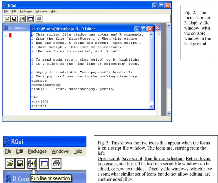
In interactive use under Microsoft Windows there are several ways to input commands to R. Figures 1 and 2 demonstrate two of the possibilities. Either or both of the following may be used at the user’s discretion. This document mostly assumes that users will type commands into the command window, at the command line prompt. Figure 1 shows the command window as it appears when version 2.0.0 of R has just been started.
The command line prompt, i.e. the >, is an invitation to start typing in your commands. For example, type 2+2
and press the Enter key. Here is what appears on the screen:
> 2+2 [1] 4 >
Here the result is 4. The[1] says, a little strangely, “first requested element will follow”. Here, there is just one element. The > indicates that R is ready for another command.
2
This is a shortcut for “right click, then left click on the copy menu item”. 3
Enter the name of your choice into the name field. For ease of remembering, choose a name that closely matches the name of the workspace directory, perhaps the name itself.
For later reference, note that the exit or quit command is
> q()
Alternatives to the use of q() are to click on the File menu and then on Exit, or to click on the in the top right hand corner of the R window. There will be a message asking whether to save the workspace image. Clicking
Yes (the safe option) will save all the objects that remain in the workspace – any that were there at the start of the session and any that have been added since.
1.2 Use of an Editor Script Window
The screen snapshot in Figure2 shows a script file window. This allows input to R of statements from a file that has been set up in advance, or that have been typed or copied into the window. To get a script file window, go to the File menu. If a new blank window is required, click on New script. To load an existing file, click on
Open script…; you will be asked for the name of a file whose contents are then displayed in the window. In Figure 2 the file was firstSteps.R.
Highlight the commands that are intended for input to R. Click on the `Run line or selection’ icon, which is the middle icon of the script file editor toolbar in Figs. 2 and 3, to send commands to R.
Under Unix, the standard form of input is the command line interface. Under both Microsoft Windows and Linux (or Unix), a further possibility is to run R from within the emacs editor4. Under Microsoft Windows,
4
This requires emacs, and ESS which runs under emacs. Both are free. Look under Software|Other on the CRAN page.
Fig. 2: The focus is on an R display file window, with the console window in the background.
Fig. 3: This shows the five icons that appear when the focus is on a script file window. The icons are, starting from the left:
attractive options are to use either the R-WinEdt utility that is designed for use with the shareware WinEdt editor, or to use the free tinn-R editor5.
1.3 A Short R Session
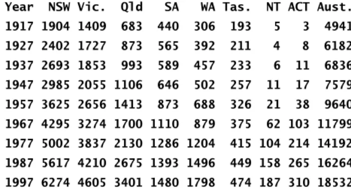
We will read into R a file that holds population figures for Australian states and territories, and total population, at various times since 1917, then using this file to create a graph. The data in the file are:
Year NSW Vic. Qld SA WA Tas. NT ACT Aust. 1917 1904 1409 683 440 306 193 5 3 4941 1927 2402 1727 873 565 392 211 4 8 6182 1937 2693 1853 993 589 457 233 6 11 6836 1947 2985 2055 1106 646 502 257 11 17 7579 1957 3625 2656 1413 873 688 326 21 38 9640 1967 4295 3274 1700 1110 879 375 62 103 11799 1977 5002 3837 2130 1286 1204 415 104 214 14192 1987 5617 4210 2675 1393 1496 449 158 265 16264 1997 6274 4605 3401 1480 1798 474 187 310 18532
The following reads in the data from the file austpop.txt on a disk in drive d: > austpop <- read.table(“d:/austpop.txt”, header=TRUE)
The <- is a left diamond bracket (<) followed by a minus sign (-). It means “is assigned to”. Use of
header=TRUE causes R to use= the first line to get header information for the columns. If column headings are not included in the file, the argument can be omitted.
Now type in austpopat the command line prompt, displaying the object on the screen:
> austpop
Year NSW Vic. Qld SA WA Tas. NT ACT Aust. 1 1917 1904 1409 683 440 306 193 5 3 4941 2 1927 2402 1727 873 565 392 211 4 8 6182 . . .
The object austpop is, in R parlance, a data frame. Data frames that consist entirely of numeric data have the same form of rectangular layout as numeric matrices. Here is a plot (Figure 4) of the Australian Capital Territory (ACT) population between 1917 and 1997 (Figure 4).
We first of all remind ourselves of the column names:
> names(austpop)
[1] "Year" "NSW" "Vic." "Qld" "SA" "WA" "Tas." "NT" [9] "ACT" "Aust."
Note that in the version of the dataset that is in the DAAG package, year has a lower case y.
5
The R-WinEdt utility, which is free, is a “plugin” for WinEdt. For links to the relevant web pages, for WinEdt R-WinEdt and various other editors that work with R, look under Software|Other on the CRAN web page.
Figure 4: Population of Australian Capital Territory, at various times between 1917 and 1997. Code to plot the graph is:
A simple way to get the plot is:
> plot(ACT ~ Year, data=austpop, pch=16) # For the DAAG version, replace ‘Year’ by ‘year’
The option pch=16 sets the plotting character to a solid black dot.
This plot can be improved greatly. We can specify more informative axis labels, change size of the text and of the plotting symbol, and so on.
1.3.1 Entry of Data at the Command Line
A data frame is a rectangular array of columns of data. Here we will have two columns, and both columns will be numeric. The following data gives, for each amount by which an elastic band is stretched over the end of a ruler, the distance that the band moved when released:
stretch 46 54 48 50 44 42 52
distance 148 182 173 166 109 141 166
The function data.frame() can be used to input these (or other) data directly at the command line. We will give the data frame the name elasticband:
elasticband <- data.frame(stretch=c(46,54,48,50,44,42,52), distance=c(148,182,173,166,109,141,166))
1.3.2 Entry and/or editing of data in an editor window
To edit the data frame elasticband in a spreadsheet-like format, type
elasticband <- edit(elasticband)
1.3.3 Options for read.table()
The function read.table() takes, optionally various parameters additional to the file name that holds the data. Specify header=TRUE if there is an initial row of header names. The default is header=FALSE. In addition users can specify the separator character or characters. Command alternatives to the default use of a space are sep="," and sep="\t". This last choice makes tabs separators. Similarly, users can control over the choice of missing value character or characters, which by default is NA. If the missing value character is a period (“.”), specify na.strings=".".
There are several variants of read.table() that differ only in having different default parameter settings. Note in particular read.csv(), which has settings that are suitable for comma delimited (csv) files that have been generated from Excel spreadsheets.
If read.table() detects that lines in the input file have different numbers of fields, data input will fail, with an error message that draws attention to the discrepancy. It is then often useful to use the function
count.fields() to report the number of fields that were identified on each separate line of the file. Figure 5: Editor window, showing the data frame
1.3.4 Options for plot() and allied functions
The function plot() and related functions accept parameters that control the plotting symbol, and the size and colour of the plotting symbol. Details will be given in Section 3.3.
1.4 Further Notational Details
As noted earlier, the command line prompt is>
R commands (expressions) are typed following this prompt6.
There is also a continuation prompt, used when, following a carriage return, the command is still not complete. By default, the continuation prompt is
+
In these notes, we often continue commands over more than one line, but omit the + that will appear on the commands window if the command is typed in as we show it.
For the names of R objects or commands, case is significant. Thus Austpop is different from austpop. For file names however, the Microsoft Windows conventions apply, and case does not distinguish file names. On Unix systems letters that have a different case are treated as different.
Anything that follows a # on the command line is taken as comment and ignored by R.
Note: Recall that, in order to quit from the R session we had to type q(). This is because q is a function. Typing q on its own, without the parentheses, displays the text of the function on the screen. Try it!
1.5 On-line Help
To get a help window (under R for Windows) with a list of help topics, type:
> help()
In R for Windows, an alternative is to click on the help menu item, and then use key words to do a search. To get help on a specific R function, e.g. plot(), type in
> help(plot)
The two search functions help.search() and apropos() can be a huge help in finding what one wants. Examples of their use are:
> help.search("matrix")
(This lists all functions whose help pages have a title or alias in which the text string “matrix” appears.)
> apropos(“matrix”)
(This lists all function names that include the text “matrix”.)
The function help.start() opens a browser window that gives access to the full range of documentation for syntax, packages and functions.
Experimentation often helps clarify the precise action of an R function.
1.6 The Loading or Attaching of Datasets
The recommended way to access datasets that are supplied for use with these notes is to attach the file
usingR.RData., available from the author's web page. Place this file in the working directory and,
from within the R session, type:
> attach("usingR.RData")
Files that are mentioned in these notes, and that are not supplied with R (e.g., from the
datasets
or
MASS
packages) should then be available without need for any further action.
6
Users can also load (use load()) or attach (use attach()) specific files. These have a similar
effect, the difference being that with attach() datasets are loaded into memory only when required
for use.
Distinguish between the attaching of image files and the attaching of data frames. The attaching of
data frames will be discussed later in these notes.
1.7 Exercises
1. In the data frame elasticband from section 1.3.1, plot distance against stretch.
2. The following ten observations, taken during the years 1970-79, are on October snow cover for Eurasia. (Snow cover is in millions of square kilometers):
year snow.cover 1970 6.5
1971 12.0 1972 14.9 1973 10.0 1974 10.7 1975 7.9 1976 21.9 1977 12.5 1978 14.5 1979 9.2
i. Enter the data into R. [Section 1.3.1 showed one way to do this. To save keystrokes, enter the successive years as 1970:1979]
ii. Plot snow.cover versus year.
iii Use the hist() command to plot a histogram of the snow cover values. iv. Repeat ii and iii after taking logarithms of snow cover.
3. Input the following data, on damage that had occurred in space shuttle launches prior to the disastrous launch of Jan 28 1986. These are the data, for 6 launches out of 24, that were included in the pre-launch charts that were used in deciding whether to proceed with the launch. (Data for the 23 launches where information is available is in the data set orings, from the DAAG package.)
Temperature Erosion Blowby Total (F) incidents incidents incidents
53 3 2 5
57 1 0 1
63 1 0 1
70 1 0 1
70 1 0 1
75 0 2 1
Enter these data into a data frame, with (for example) column names temperature, erosion, blowby and
2. An Overview of R
2.1 The Uses of R
2.1.1 R may be used as a calculator.
R evaluates and prints out the result of any expression that one types in at the command line in the console window. Expressions are typed following the prompt (>) on the screen. The result, if any, appears on subsequent lines
> 2+2 [1] 4 > sqrt(10) [1] 3.162278 > 2*3*4*5 [1] 120
> 1000*(1+0.075)^5 - 1000 # Interest on $1000, compounded annually [1] 435.6293
> # at 7.5% p.a. for five years > pi # R knows about pi
[1] 3.141593
> 2*pi*6378 #Circumference of Earth at Equator, in km; radius is 6378 km [1] 40074.16
> sin(c(30,60,90)*pi/180) # Convert angles to radians, then take sin() [1] 0.5000000 0.8660254 1.0000000
2.1.2 R will provide numerical or graphical summaries of data
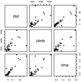
A special class of object, called a data frame, stores rectangular arrays in which the columns may be vectors of numbers or factors or text strings. Data frames are central to the way that all the more recent R routines process data. For now, think of data frames as matrices, where the rows are observations and the columns are variables. As a first example, consider the data frame hills that accompanies these notes7. This has three columns
(variables), with the names distance, climb, and time. Typing in summary(hills)gives summary information on these variables. There is one column for each variable, thus:
> load("hills.Rdata") # Assumes hills.Rdata is in the working directory > summary(hills)
distance climb time Min.: 2.000 Min.: 300 Min.: 15.95 1st Qu.: 4.500 1st Qu.: 725 1st Qu.: 28.00 Median: 6.000 Median:1000 Median: 39.75 Mean: 7.529 Mean:1815 Mean: 57.88 3rd Qu.: 8.000 3rd Qu.:2200 3rd Qu.: 68.62 Max.:28.000 Max.:7500 Max.:204.60
We may for example require information on ranges of variables. Thus the range of distances (first column) is from 2 miles to 28 miles, while the range of times (third column) is from 15.95 (minutes) to 204.6 minutes. We will discuss graphical summaries in the next section.
7
2.1.3 R has extensive graphical abilities
The main R graphics function is plot(). In addition to plot() there are functions for adding points and lines to existing graphs, for placing text at specified positions, for specifying tick marks and tick labels, for labelling axes, and so on.
There are various other alternative helpful forms of graphical summary. A helpful graphical summary for the
hills data frame is the scatterplot matrix, shown in Figure 5. For this, type:
> pairs(hills)
Figure 5: Scatterplot matrix for the Scottish hill race data
2.1.4 R will handle a variety of specific analyses
The examples that will be given are correlation and regression.
Correlation:
We calculate the correlation matrix for the hills data:
> options(digits=3) > cor(hills)
distance climb time distance 1.000 0.652 0.920 climb 0.652 1.000 0.805 time 0.920 0.805 1.000
Suppose we wish to calculate logarithms, and then calculate correlations. We can do all this in one step, thus:
> cor(log(hills))
distance climb time distance 1.00 0.700 0.890 climb 0.70 1.000 0.724 time 0.89 0.724 1.000
Unfortunately R was not clever enough to relabel distance as log(distance), climb as log(climb), and time as log(time). Notice that the correlations between time and distance, and between time and climb, have reduced. Why has this happened?
Straight Line Regression:
Here is a straight line regression calculation. The data are stored in the data frame elasticband (DAAG package). The variable names are the names of columns in that data frame. The formula that is supplied to the
> plot(distance ~ stretch,data=elasticband, pch=16) > elastic.lm <- lm(distance~stretch,data=elasticband) > lm(distance ~stretch,data=elasticband)
Call:
lm(formula = distance ~ stretch, data = elasticband)
Coefficients:
(Intercept) stretch -63.571 4.554
More complete information is available by typing
> summary(lm(distance~stretch,data=elasticband))
Try it!
2.1.5 R is an Interactive Programming Language
We calculate the Fahrenheit temperatures that correspond to Celsius temperatures 25, 26, …, 30:
> celsius <- 25:30
> fahrenheit <- 9/5*celsius+32
> conversion <- data.frame(Celsius=celsius, Fahrenheit=fahrenheit) > print(conversion)
Celsius Fahrenheit 1 25 77.0 2 26 78.8 3 27 80.6 4 28 82.4 5 29 84.2 6 30 86.0
2.2 R Objects
All R entities, including functions and data structures, exist as objects. They can all be operated on as data. Type in ls() to see the names of all objects in your workspace. An alternative to ls() is objects(). In both cases there is provision to specify a particular pattern, e.g. starting with the letter `p’8.
Typing the name of an object causes the printing of its contents. Try typing q, mean, etc.
In a long session, it makes sense to save the contents of the working directory from time to time. It is also possible to save individual objects, or collections of objects into a named image file. Some possibilities are:
save.image() # Save contents of workspace, into the file .RData save.image(file="archive.RData") # Save into the file archive.RData
save(celsius, fahrenheit, file="tempscales.RData")
Image files, from the working directory or (with the path specified) from another directory, can be attached, thus making objects in the file available on request. For example
attach("tempscales.RData")
ls(pos=2) # Check the contents of the file that has been attached
The parameter pos gives the position on the search list. (The search list is discussed later in this chapter, in Section 2.9.)
Important: On quitting, R offers the option of saving the workspace image, by default in the file .RData in the working directory. This allows the retention, for use in the next session in the same workspace, any objects that were created in the current session. Careful housekeeping may be needed to distinguish between objects that are
8
to be kept and objects that will not be used again. Before typing q() to quit, use rm() to remove objects that are no longer required. Saving the workspace image will then save everything remains. The workspace image will be automatically loaded upon starting another session in that directory.
*
92.3 Looping
A simple example of a for loop is10
for (i in 1:10) print(i)
Here is another example of a for loop, to do in a complicated way what we did very simply in section 2.1.5:
> # Celsius to Fahrenheit > for (celsius in 25:30)
+ print(c(celsius, 9/5*celsius + 32)) [1] 25 77
[1] 26.0 78.8 [1] 27.0 80.6 [1] 28.0 82.4 [1] 29.0 84.2 [1] 30 86
2.3.1 More on looping
Here is a long-winded way to sum the three numbers 31, 51 and 91:
> answer <- 0
> for (j in c(31,51,91)){answer <- j+answer} > answer
[1] 173
The calculation iteratively builds up the object answer, using the successive values of j listed in the vector (31,51,91). i.e. Initially, j=31, and answer is assigned the value 31 + 0 = 31. Then j=51, and answer is assigned the value 51 + 31 = 82. Finally, j=91, and answer is assigned the value 91 + 81 = 173. Then the procedure ends, and the contents of answer can be examined by typing in answer and pressing the Enter key. There is a more straightforward way to do this calculation:
> sum(c(31,51,91)) [1] 173
Skilled R users have limited recourse to loops. There are often, as in this and earlier examples, better alternatives.
2.4 Vectors
Examples of vectors arec(2,3,5,2,7,1)
3:10 # The numbers 3, 4, .., 10
c(TRUE,FALSE,FALSE,FALSE,TRUE,TRUE,FALSE) c(”Canberra”,”Sydney”,”Newcastle”,”Darwin”)
Vectors may have mode logical, numeric or character11. The first two vectors above are numeric, the third is
logical (i.e. a vector with elements of mode logical), and the fourth is a string vector (i.e. a vector with elements of mode character).
9
Asterisks (*) identify sections that are more technical and might be omitted at a first reading 10
Other looping constructs are:
repeat <expression> ## break must appear somewhere inside the loop while (x>0) <expression>
The missing value symbol, which is NA, can be included as an element of a vector.
2.4.1 Joining (concatenating) vectors
The c in c(2, 3, 5, 7, 1) above is an acronym for “concatenate”, i.e. the meaning is: “Join these numbers together in to a vector. Existing vectors may be included among the elements that are to be concatenated. In the following we form vectors x and y, which we then concatenate to form a vector z:
> x <- c(2,3,5,2,7,1) > x
[1] 2 3 5 2 7 1 > y <- c(10,15,12) > y
[1] 10 15 12
> z <- c(x, y) > z
[1] 2 3 5 2 7 1 10 15 12
The concatenate function c() may also be used to join lists.
2.4.2 Subsets of Vectors
There are two common ways to extract subsets of vectors12. 1. Specify the numbers of the elements that are to be extracted, e.g.
> x <- c(3,11,8,15,12) # Assign to x the values 3, 11, 8, 15, 12 > x[c(2,4)] # Extract elements (rows) 2 and 4
[1] 11 15
One can use negative numbers to omit elements:
> x <- c(3,11,8,15,12) > x[-c(2,3)]
[1] 3 15 12
2. Specify a vector of logical values. The elements that are extracted are those for which the logical value is T. Thus suppose we want to extract values of x that are greater than 10.
> x>10 # This generates a vector of logical (T or F) [1] F T F T T
> x[x>10] [1] 11 15 12
Arithmetic relations that may be used in the extraction of subsets of vectors are <, <=, >, >=, ==, and !=. The first four compare magnitudes, == tests for equality, and != tests for inequality.
2.4.3 The Use of NA in Vector Subscripts
Note that any arithmetic operation or relation that involves NA generates an NA. Set
y <- c(1, NA, 3, 0, NA)
11 It will, later in these notes, be important to know the “class” of such objects. This determines how the
method used by such generic functions as print(), plot() and summary(). Use the function class()
to determine the class of an object.
12 A third more subtle method is available when vectors have named elements. One can then use a vector of
names to extract the elements, thus:
> c(Andreas=178, John=185, Jeff=183)[c("John","Jeff")] John Jeff
Be warned that y[y==NA] <- 0 leaves y unchanged. The reason is that all elements of y==NA evaluate to NA. This does not select an element of y, and there is no assignment.
To replace all NAs by 0, use
y[is.na(y)] <- 0
2.4.4 Factors
A factor is stored internally as a numeric vector with values 1, 2, 3, k, where k is the number of levels. An attributes table gives the ‘level’ for each integer value13. Factors provide a compact way to store character
strings. They are crucial in the representation of categorical effects in model and graphics formulae. The class attribute of a factor has, not surprisingly, the value “factor”.
Consider a survey that has data on 691 females and 692 males. If the first 691 are females and the next 692 males, we can create a vector of strings that that holds the values thus:
gender <- c(rep(“female”,691), rep(“male”,692))
(The usage is that rep(“female”, 691) creates 691 copies of the character string “female”, and similarly for the creation of 692 copies of “male”.)
We can change the vector to a factor, by entering:
gender <- factor(gender)
Internally the factor gender is stored as 691 1’s, followed by 692 2’s. It has stored with it the table:
1
female2 male
Once stored as a factor, the space required for storage is reduced.
In most cases where the context seems to demand a character string, the 1 is translated into “female” and the 2 into “male”. The values “female” and “male” are the levels of the factor. By default, the levels are in
alphanumeric order, so that “female” precedes “male”. Hence:
> levels(gender) # Assumes gender is a factor, created as above [1] "female" "male"
The order of the levels in a factor determines the order in which the levels appear in graphs that use this information, and in tables. To cause “male” to come before “female”, use
gender <- relevel(gender, ref=“male”)
An alternative is
gender <- factor(gender, levels=c(“male”, “female”))
This last syntax is available both when the factor is first created, or later when one wishes to change the order of levels in an existing factor. Incorrect spelling of the level names will generate an error message. Try
gender <- factor(c(rep(“female”,691), rep(“male”,692))) table(gender)
gender <- factor(gender, levels=c(“male”, “female”)) table(gender)
gender <- factor(gender, levels=c(“Male”, “female”))
# Erroneous - "male" rows now hold missing values table(gender)
rm(gender) # Remove gender
13
The attributes() function makes it possible to inspect attributes. For example attributes(factor(1:3))
2.5 Data Frames
Data frames are fundamental to the use of the R modelling and graphics functions. A data frame is a
generalisation of a matrix, in which different columns may have different modes. All elements of any column must however have the same mode, i.e. all numeric or all factor, or all character.
Among the data sets in the DAAG package is Cars93.summary, created from information in the Cars93 data set in the Venables and Ripley MASS package. Here it is:
> Cars93.summary
Min.passengers Max.passengers No.of.cars abbrev Compact 4 6 16 C Large 6 6 11 L Midsize 4 6 22 M Small 4 5 21 Sm Sporty 2 4 14 Sp Van 7 8 9 V
The data frame has row labels (access with row.names(Cars93.summary)) Compact, Large, . . . The column names (access with names(Cars93.summary)) are Min.passengers (i.e. the minimum number of
passengers for cars in this category), Max.passengers, No.of.cars., and abbrev. The first three columns have mode numeric, and the fourth has mode character. Columns can be vectors of any mode. The column
abbrev could equally well be stored as a factor.
Any of the following14 will pick out the fourth column of the data frame Cars93.summary, then storing it in
the vector type.
type <- Cars93.summary$abbrev type <- Cars93.summary[,4]
type <- Cars93.summary[,”abbrev”]
type <- Cars93.summary[[4]] # Take the object that is stored # in the fourth list element.
2.5.1 Data frames as lists
A data frame is a list15 of column vectors, all of equal length. Just as with any other list, subscripting extracts a
list. Thus Cars93.summary[4] is a data frame with a single column, which is the fourth column vector of
Cars93.summary. As noted above, use Cars93.summary[[4]] or Cars93.summary[,4] to extract the column vector.
The use of matrix-like subscripting, e.g. Cars93.summary[,4] or Cars93.summary[1, 4], takes advantage of the rectangular structure of data frames.
2.5.2 Inclusion of character string vectors in data frames
When data are input using read.table(), or when the data.frame() function is used to create data frames, vectors of character strings are by default turned into factors. The parameter setting
stringsAsFactors=TRUE, available both with read.table() and with data.frame(), will if needed ensure that character strings are input without such conversion. For read.table(), an alternative is
as.is=TRUE.
2.5.3 Built-in data sets
We will often use data sets that accompany one of the R packages, usually stored as data frames. One such data frame, in the datasets package, is trees, which gives girth, height and volume for 31 Black Cherry Trees.
Here is summary information on this data frame
14
Also legal is Cars93.summary[2]. This gives a data frame with the single column Type. 15
> summary(trees)
Girth Height Volume Min. : 8.30 Min. :63 Min. :10.20 1st Qu.:11.05 1st Qu.:72 1st Qu.:19.40 Median :12.90 Median :76 Median :24.20 Mean :13.25 Mean :76 Mean :30.17 3rd Qu.:15.25 3rd Qu.:80 3rd Qu.:37.30 Max. :20.60 Max. :87 Max. :77.00
Type data() to get a list of built-in data sets in the packages that have been attached16.
2.6 Common Useful Functions
print() # Prints a single R object
cat() # Prints multiple objects, one after the other length() # Number of elements in a vector or of a list mean()
median() range()
unique() # Gives the vector of distinct values
diff() # Replace a vector by the vector of first differences # N. B. diff(x) has one less element than x
sort() # Sort elements into order, but omitting NAs order() # x[order(x)] orders elements of x, with NAs last cumsum()
cumprod()
rev() # reverse the order of vector elements
The functions mean(), median(), range(), and a number of other functions, take the argument na.rm=T;
i.e. remove NAs, then proceed with the calculation.
By default, sort() omits any NAs. The function order() places NAs last. Hence:ƒ
> x <- c(1, 20, 2, NA, 22) > order(x)
[1] 1 3 2 5 4 > x[order(x)] [1] 1 2 20 22 NA > sort(x)
[1] 1 2 20 22
2.6.1 Applying a function to all columns of a data frame
The function sapply() takes as arguments the the data frame, and the function that is to be applied. The following applies the function is.factor() to all columns of the supplied data frame rainforest17.
> sapply(rainforest, is.factor)
dbh wood bark root rootsk branch species FALSE FALSE FALSE FALSE FALSE FALSE TRUE
> sapply(rainforest[,-7], range) # The final column (7) is a factor dbh wood bark root rootsk branch
[1,] 4 NA NA NA NA NA [2,] 56 NA NA NA NA NA
16
The list include all packages that are in the current environment. 17
The functions mean() and range(), and a number of other functions, take the parameter na.rm. For example > range(rainforest$branch, na.rm=TRUE) # Omit NAs, then determine the range [1] 4 120
One can specify na.rm=TRUE as a third argument to the function sapply. This argument is then automatically passed to the function that is specified in the second argument position. For example:
> sapply(rainforest[,-7], range, na.rm=TRUE) dbh wood bark root rootsk branch [1,] 4 3 8 2 0.3 4 [2,] 56 1530 105 135 24.0 120
Chapter 8 has further details on the use of sapply(). There is an example that shows how to use it to count the number of missing values in each column of data.
2.7 Making Tables
table() makes a table of counts. Specify one vector of values (often a factor) for each table margin that is required. For example:
> library(lattice) # The data frame barley accompanies lattice > table(barley$year, barley$site)
Grand Rapids Duluth University Farm Morris Crookston Waseca 1932 10 10 10 10 10 10 1931 10 10 10 10 10 10
WARNING: NAs are by default ignored. The action needed to get NAs tabulated under a separate NA category depends, annoyingly, on whether or not the vector is a factor. If the vector is not a factor, specify
exclude=NULL. If the vector is a factor then it is necessary to generate a new factor that includes “NA” as a level. Specify x <- factor(x,exclude=NULL)
> x <- c(1,5,NA,8) > x <- factor(x) > x
[1] 1 5 NA 8 Levels: 1 5 8
> factor(x,exclude=NULL) [1] 1 5 NA 8
Levels: 1 5 8 NA
2.7.1 Numbers of NAs in subgroups of the data
The following gives information on the number of NAs in subgroups of the data:
> table(rainforest$species, !is.na(rainforest$branch))
FALSE TRUE Acacia mabellae 6 10 C. fraseri 0 12 Acmena smithii 15 11 B. myrtifolia 1 10
Thus for Acacia mabellae there are 6 NAs for the variable branch (i.e. number of branches over 2cm in diameter), out of a total of 16 data values.
2.8 The Search List
R has a search list where it looks for objects. This can be changed in the course of a session. To get a full list of these directories, called databases, type:
> search()
[4] "package:graphics" "package:grDevices" "package:utils" [7] "package:datasets" "Autoloads" "package:base"
Notice that the loading of a new package extends the search list.
> library(MASS) > search()
[1] ".GlobalEnv" "package:MASS" "package:methods" [4] "package:stats" "package:graphics" "package:grDevices" [7] "package:utils" "package:datasets" "Autoloads" [10] "package:base"
Use of attach() likewise extends the search list.This function can be used to attach data frames or lists (use the name, without quotes) or image (.RData) files (the file name is placed in quotes).
The following demonstrates the attaching of the data frame primates:
> names(primates) [1] "Bodywt" "Brainwt" > Bodywt
Error: Object "Bodywt" not found
> attach(primates) # R will now know where to find Bodywt > Bodywt
[1] 10.0 207.0 62.0 6.8 52.2
Once the data frame primates has been attached, its columns can be accessed by giving their names, without further reference to the name of the data frame. In technical terms, the data frame becomes a database, which is searched as required for objects that the user may specify. Remember to detach an attached data frame, e.g.,
detach(primates), when it is no longer required.
Note also the function with(), which attaches the data frame that is given as its first argument for the duration of the calculation that is specified by its second argument. For example:
> av <- with(primates, mean(Bodywt))
2.9 Functions in R
We give two simple examples of R functions.
2.9.1 An Approximate Miles to Kilometers Conversion
miles.to.km <- function(miles)miles*8/5The return value is the value of the final (and in this instance only) expression that appears in the function body18. Use the function thus
> miles.to.km(175) # Approximate distance to Sydney, in miles [1] 280
The function will do the conversion for several distances all at once. To convert a vector of the three distances 100, 200 and 300 miles to distances in kilometers, specify:
> miles.to.km(c(100,200,300)) [1] 160 320 480
2.9.2 A Plotting function
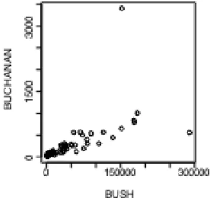
The data set florida has the votes in the 2000 election for the various US Presidential candidates, county by county in the state of Florida. The following plots the vote for Buchanan against the vote for Bush.
attach(florida)
plot(BUSH, BUCHANAN, xlab="Bush", ylab="Buchanan") detach(florida) # In S-PLUS, specify detach("florida")
18
Here is a function that makes it possible to plot the figures for any pair of candidates.
plot.florida <- function(xvar=”BUSH”, yvar=”BUCHANAN”){ x <- florida[,xvar]
y <- florida[,yvar]
plot(x, y, xlab=xvar,ylab=yvar) mtext(side=3, line=1.75,
“Votes in Florida, by county, in \nthe 2000 US Presidential election”) }
Note that the function body is enclosed in braces ({ }).
Figure 6 shows the graph produced by plot.florida(),i.e. parameter settings are left at their defaults.
Figure 6: Election night count of votes received, by county, in the US 2000 Presidential election.
As well as plot.florida(), the function allows, e.g.
plot.florida(yvar=”NADER”) # yvar=”NADER” over-rides the default plot.florida(xvar=”GORE”, yvar=”NADER”)
2.10 More Detailed Information
Chapters 7 and 8 have a more detailed coverage of the topics in this chapter. It may pay, at this point, to glance through chapters 7 and 8. Remember also to use R’s help pages and functions.
Topics from chapter 7, additional to those covered above, that may be important for relatively elementary uses of R include:
The entry of patterned data (7.1.3)
The handling of missing values in subscripts when vectors are assigned (7.2)
Unexpected consequences (e.g. conversion of columns of numeric data into factors) from errors in data (7.4.1).
2.11 Exercises
1. For each of the following code sequences, predict the result. Then do the computation: a) answer <- 0
for (j in 3:5){ answer <- j+answer }
b) answer<- 10
for (j in 3:5){ answer <- j+answer }
c) answer <- 10
for (j in 3:5){ answer <- j*answer }
2. Look up the help for the function prod(), and use prod() to do the calculation in 1(c) above. Alternatively, how would you expect prod() to work? Try it!
4. Multiply all the numbers from 1 to 50 in two different ways: using for and using prod.
5. The volume of a sphere of radius r is given by 4 r3/3. For spheres having radii 3, 4, 5, …, 20 find the
corresponding volumes and print the results out in a table. Use the technique of section 2.1.5 to construct a data frame with columns radius and volume.
3. Plotting
The functions plot(), points(), lines(), text(), mtext(), axis(), identify() etc. form a suite that plots points, lines and text. To see some of the possibilities that R offers, enter
demo(graphics)
Press the Enter key to move to each new graph.
3.1 plot () and allied functions
The following both plot y against x:plot(y ~ x) # Use a formula to specify the graph plot(x, y) #
Obviously x and y must be the same length. Try
plot((0:20)*pi/10, sin((0:20)*pi/10)) plot((1:30)*0.92, sin((1:30)*0.92))
Comment on the appearance that these graphs present. Is it obvious that these points lie on a sine curve? How can one make it obvious? (Place the cursor over the lower border of the graph sheet, until it becomes a double-sided arror. Drag the border in towards the top border, making the graph sheet short and wide.)
Here are two further examples.
attach(elasticband) # R now knows where to find distance & stretch plot(distance ~ stretch)
plot(ACT ~ Year, data=austpop, type="l") plot(ACT ~ Year, data=austpop, type="b")
The points() function adds points to a plot. The lines()function adds lines to a plot19. The text()
function adds text at specified locations. The mtext() function places text in one of the margins. The axis()
function gives fine control over axis ticks and labels. Here is a further possibility
attach(austpop)
plot(spline(Year, ACT), type="l") # Fit smooth curve through points detach(austpop) # In S-PLUS, specify detach(“austpop”)
3.1.1 Plot methods for other classes of object
The plot function is a generic function that has special methods for “plotting” various different classes of object. For example, plotting a data frame gives, for each numeric variable, a normal probability plot. Plotting the lm
object that is created by the use of the lm() modelling function gives diagnostic and other information that is intended to help in the interpretation of regression results.
Try
plot(hills) # Has the same effect as pairs(hills)
3.2 Fine control – Parameter settings
The default settings of parameters, such as character size, are often adequate. When it is necessary to change parameter settings for a subsequent plot, the par() function does this. For example,
par(cex=1.25) # character expansion
increases the text and plot symbol size 25% above the default.
19 Actually these functions differ only in the default setting for the parameter
type. The default setting for
On the first use of par() to make changes to the current device, it is often useful to store existing settings, so that they can be restored later. For this, specify
oldpar <- par(cex=1.25, mex=1.25) # mex=1.25 expands the margin by 25%
This stores the existing settings in oldpar, then changes parameters (here cex and mex) as requested. To restore the original parameter settings at some later time, enter par(oldpar). Here is an example:
attach(elasticband) oldpar <- par(cex=1.5) plot(distance ~ stretch)
par(oldpar) # Restores the earlier settings detach(elasticband)
Inside a function specify, e.g.
oldpar <- par(cex=1.25) on.exit(par(oldpar))
Type in help(par) to get details of all the parameter settings that are available with par().
3.2.1 Multiple plots on the one page
The parameter mfrow can be used to configure the graphics sheet so that subsequent plots appear row by row, one after the other in a rectangular layout, on the one page. For a column by column layout, use mfcol instead. In the example below we present four different transformations of the primates data, in a two by two layout:
par(mfrow=c(2,2), pch=16)
attach(Animals) # This dataset is in the MASS package, which must be attached plot(body, brain)
plot(sqrt(body), sqrt(brain)) plot((body)^0.1, (brain)^0.1) plot(log(body),log(brain)) detach(Animals)
par(mfrow=c(1,1), pch=1) # Restore to 1 figure per page
3.2.2 The shape of the graph sheet
Often it is desirable to exercise control over the shape of the graph page, e.g. so that the individual plots are rectangular rather than square. The R for Windows functions win.graph() or x11()that set up the Windows screentake the parameters width(in inches), height (in inches) and pointsize (in 1/72 of an inch). The setting of pointsize (default =12) determines character heights. It is the relative sizes of these parameters that matter for screen display or for incorporation into Word and similar programs. Graphs can be enlarged or shrunk by pointing at one corner, holding down the left mouse button, and pulling.
3.3 Adding points, lines and text
Here is a simple example that shows how to use the function text() to add text labels to the points on a plot.
> primates
Bodywt Brainwt Potar monkey 10.0 115 Gorilla 207.0 406 Human 62.0 1320 Rhesus monkey 6.8 179 Chimp 52.2 440
Observe that the row names store labels for each row20.
20
Row names can be created in several different ways. They can be assigned directly, e.g.
attach(primates) # Needed if primates is not already attached. plot(Bodywt, Brainwt)
text(x=Bodywt, y=Brainwt, labels=row.names(primates), pos=4) # pos=4 positions text to the right of the point
Figure 7A shows the result.
Figure 7: Plot of the primates data, with labels on points. Figure 8B improves on Figure 8A.
Figure 7A would be adequate for identifying points, but is not a presentation quality graph. We now show how to improve it. Figure 7B uses the xlab (x-axis) and ylab (y-axis) parameters to specify meaningful axis titles. It uses the parameter setting pos=4 to move the labelling to the right of the points. It sets pch=16 to make the plot character a heavy black dot. This helps make the points stand out against the labelling.
Here is the R code for Figure 7B:
plot(x=Bodywt, y=Brainwt, pch=16,
xlab="Body weight (kg)", ylab="Brain weight (g)", xlim=c(0,280), ylim=c(0,1350))
# Specify xlim so that there is room for the labels
text(x=Bodywt, y=Brainwt, labels=row.names(primates), pos=4) detach(primates)
To place the text to the left of the points, specify
text(x=Bodywt, y=Brainwt, labels=row.names(primates), pos=2)
3.3.1 Size, colour and choice of plotting symbol
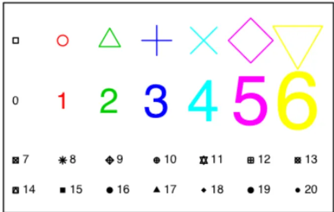
For plot() and points() the parameter cex (“character expansion”) controls the size, while col (“colour”) controls the colour of the plotting symbol. The parameter pch controls the choice of plotting symbol.
The parameters cex and col may be used in a similar way with text(). Try
plot(1, 1, xlim=c(1, 7.5), ylim=c(1.75,5), type="n", axes=F, xlab="", ylab="") # Do not plot points
box()
points(1:7, rep(4.5, 7), cex=1:7, col=1:7, pch=0:6) text(1:7,rep(3.5, 7), labels=paste(0:6), cex=1:7, col=1:7)
The following, added to the plot that results from the above three statements, demonstrates other choices of pch.
points(1:7,rep(2.5,7), pch=(0:6)+7) # Plot symbols 7 to 13 text((1:7), rep(2.5,7), paste((0:6)+7), pos=4) # Label with symbol number points(1:7,rep(2,7), pch=(0:6)+14) # Plot symbols 14 to 20
text((1:7), rep(2,7), paste((0:6)+14), pos=4) # Labels with symbol number